Embed Size (px)
Citation preview
329
Chapter 5Propagation and Scattering in a Spherical-
Stratified Refracting Medium
5.1 Introduction
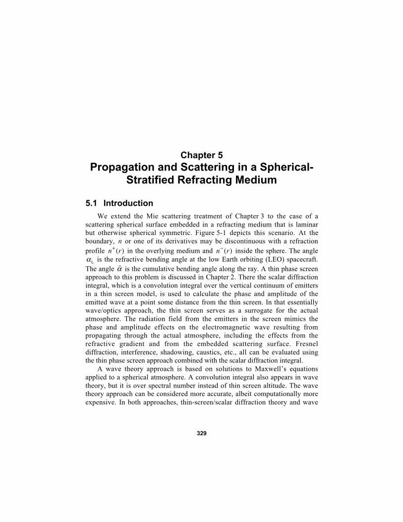
We extend the Mie scattering treatment of Chapter 3 to the case of ascattering spherical surface embedded in a refracting medium that is laminarbut otherwise spherical symmetric. Figure 5-1 depicts this scenario. At theboundary, n or one of its derivatives may be discontinuous with a refractionprofile n r+ ( ) in the overlying medium and n r− ( ) inside the sphere. The angleαL is the refractive bending angle at the low Earth orbiting (LEO) spacecraft.The angle α is the cumulative bending angle along the ray. A thin phase screenapproach to this problem is discussed in Chapter 2. There the scalar diffractionintegral, which is a convolution integral over the vertical continuum of emittersin a thin screen model, is used to calculate the phase and amplitude of theemitted wave at a point some distance from the thin screen. In that essentiallywave/optics approach, the thin screen serves as a surrogate for the actualatmosphere. The radiation field from the emitters in the screen mimics thephase and amplitude effects on the electromagnetic wave resulting frompropagating through the actual atmosphere, including the effects from therefractive gradient and from the embedded scattering surface. Fresneldiffraction, interference, shadowing, caustics, etc., all can be evaluated usingthe thin phase screen approach combined with the scalar diffraction integral.
A wave theory approach is based on solutions to Maxwell’s equationsapplied to a spherical atmosphere. A convolution integral also appears in wavetheory, but it is over spectral number instead of thin screen altitude. The wavetheory approach can be considered more accurate, albeit computationally moreexpensive. In both approaches, thin-screen/scalar diffraction theory and wave

330 Chapter 5
theory, one ends up with a prediction of the observed phase and amplitude ofthe wave at some point as a result of its passing through an interveningatmosphere and perhaps encountering an embedded scattering surface. Onequestion addressed here is the level of agreement between these twoapproaches, and how that level depends on the adversity of the wavepropagation conditions in the atmosphere.
One concludes from a review of wave propagation literature that scatteringtheory in a sphere is potentially a very complicated problem. For example, seethe survey article by Chapman and Orcutt [1] on wave propagation problems inseismology. There one finds refracted rays reflecting from multiple surfaces,Rayleigh and Love waves skittering along boundaries, super-refracted waveswith multiple reflections ducted along between layers, and so on. Here wespecifically rule out ducting, evanescence, or other confounding propagationeffects, except for the effects resulting from the class of discontinuities understudy here, which would include interference, shadow zones, caustics,diffraction, and super-refractivity. We assume that embedded in and co-centered with this refracting medium is a single large spherical scatteringsurface. Across this surface a discontinuity in the refractivity model is assumedto exist. This discontinuity can take different forms, ranging from adiscontinuity in n itself, or in its gradient, or to a discontinuity merely in one ofits higher derivatives. We must account for the effects of the refractive gradientin the overlying medium surrounding the sphere on the phase and amplitude ofthe electromagnetic wave. Therefore, scattering in this context includes externalreflection from the scattering sphere, transmission through and refraction by thescattering sphere, including the possibility that the scattered wave has
α
S
LEO
L / 2
rL
r*
To GPS
ro
˜
n + ( r ) n − ( r )
Fig. 5-1. Ray path geometry for a scattering sphere embedded in a stratified medium.The profiles for the index of refraction are given by n − ( r ) inside the sphere and byn + ( r ) outside the sphere.
α
θθ*
L

Propagation and Scattering 331
undergone one or more reflections inside the scattering sphere, and finally therefractive bending of the scattered ray from the overlying medium.
For the purpose of comparing results from the full-wave theory approachwith the scalar diffraction/thin phase screen approach, we assume that the localgradient of the refractivity is sufficiently small throughout the mediumsurrounding the scattering sphere so that the “thin atmosphere” conditions [seeSection 2.2, Eqs. (2.2-8) and (2.2-9)] apply. Where rapid changes in refractivityare encountered—for example, at the boundary of a super-refracting watervapor layer—we assume that such changes are sufficiently localized that rayoptics is still valid, i.e., rays do exist that pass through such a barrier, for atleast a certain range of tangency points.
The wave theory approach followed here is derived from Mie scatteringtheory, but it is adapted to a medium with a continuously changing refractivity.The original formulation of Mie scattering theory [2] deals with a singlespherical scattering surface in an otherwise homogeneous medium. Numericalwave theory approaches involve approximations to the solutions of Maxwell’sequations in one form or another. In this chapter, we use an osculatingparameter technique for dealing with the spectral integrals associated with wavetheory. The accuracy of such a technique and its range of applicability areimportant questions that need to be addressed. The accuracy and range ofapplicability depend on the choice of basis functions used in the osculatingparameter technique. For example, in a Cartesian-stratified medium, the use ofsinusoids as the basis functions results in an osculating parameter solution thatis identical to the Wentzel–Kramer–Brillouin (WKB) solution. The conditionsfor attaining a given accuracy and ascertaining its range of applicability arewell established for WKB solutions. There also is a wealth of literature on theconnection problem in WKB solutions across the transition zone between theoscillatory and exponential-decaying branches, important for quantumtunneling processes and other applications. Fortunately, we are concerned withthe electromagnetic field away from turning points; therefore, asymptotic formsapplicable to the oscillatory branch play an important role here. For a differentchoice of basis functions, the osculating parameter solutions do not reduce tothe WKB forms and have a different range of applicability. Here the favoredbasis functions are the spherical Bessel functions or their Airy functionsurrogates, which are asymptotically equivalent when the radius of thescattering surface is very large compared to the wavelength of theelectromagnetic wave. These particular basis functions offer a wide range ofapplicability for the osculating parameter solutions. Even at a turning point, abête noir for wave theory, these basis functions provide a useful, if notcompletely successful, approach.
The question arises concerning the many sections to follow as to whichparts are essential to this wave theory approach. Sections 5.2 and 5.3 provide abrief review of the basic general concepts in classical electrodynamics

332 Chapter 5
involving harmonic waves: Maxwell’s equations, scalar potentials forgenerating the electromagnetic field vectors, and series solutions using theseparation of variables technique. These series involve spherical harmonicfunctions, which apply for spherical symmetry, but special functions are neededfor the radial component. For the homogeneous case, these radial solutionsbecome the spherical Bessel functions, but in general the radial functionsdepend on the refractivity profile of the medium. It is here that techniques likethe WKB method or the osculating parameter technique arise.
Section 5.4 briefly summarizes the asymptotic approximations that are usedin this chapter. A fuller account is found in Section 3.8. This section is referredto frequently in the later text.
Section 5.5 begins the adaptation of Mie scattering theory from a singlelarge spherical surface to a concatenated series of concentric layers that in theirlimiting form approach a medium with a continuously varying refractivity. Thissection introduces a spectral density function for the phase delay induced by therefractive gradient in the medium. This quantity (defined as G[ , ]ρ ν in thatsection) essentially accounts for the extra phase delay at the radial position ρexperienced by a radial wave component of integer spectral numberl = −ν 1 2/ , which results from the refractive gradient of the medium. In ahomogeneous medium, G[ , ]ρ ν ≡ 0 . We consider there the propagation of anincident wave that asymptotically is planar at large approaching distancesrelative to the scattering sphere. The adjustments to account for a sphericalapproaching wave (when the emitting Global Positioning System (GPS)satellite is placed only a finite distance away) are noted.
Section 5.6 reviews several important concepts from geometric optics thatare needed later when correspondences are established between these conceptsand certain properties from wave theory when the spectral number assumes astationary phase value. Geometric optics is discussed in Appendix A, but here,in addition to discussing the stationary phase property of a ray and its bendingangle and phase delay, this section also introduces the concept of a cumulativebending angle along the ray, which mainly arises when evaluating theelectromagnetic field within the refractive medium. This section also discussesBouguer’s law and the impact parameter of a ray, the geometric opticsequivalent of the conservation of angular momentum in a conservative forcefield. This section also covers defocusing and the first Fresnel zone. Limitationsin second-order geometric optics, which arise in association with caustics orwhen two or more rays have impact parameter separations that are less than thefirst Fresnel zone, are discussed in Section 5.12.
Section 5.7 develops more asymptotic forms needed later. The ratio of theradius of curvature of the stratified surface to the wavelength of the incidentwave, ro / λ , is sufficiently large that asymptotic forms for the Bessel functionsapply. Also, because only spectral numbers that are of the same order of

Propagation and Scattering 333
magnitude as ro / λ contribute significantly to the spectral integralsrepresenting the field, we also can use the asymptotic forms for the harmonicfunctions that apply for large spectral number. Section 5.7 shows the closecorrespondence between certain geometric optics quantities—for example, thecumulative bending angle of a ray with an impact parameter value, ν , andevaluated at a radial position, ρ , and a certain spectral quantity from wavetheory, ∂ ρ ν ∂νG[ , ] / . The issue of a breakdown in accuracy of the osculatingparameter technique near a turning point ν ρ= also is addressed here. Thebehavior of the WKB solutions near a turning point is used to provide guidancein dealing with this breakdown. An asymptotic matching technique isdeveloped to set the value of G[ , ]ρ ν for the regime ν ρ> .
Section 5.8 begins the representation of the electromagnetic field in termsof the spectral integrals involving the spectral components of the radialosculating parameter functions and the harmonic functions for the anglecoordinates.
This discussion is continued in Section 5.9, where a phasor representationfor the integrands in these spectral integrals is introduced. The stationary phasetechnique also is introduced here. It is used to determine spectral number pointsthat yield stationary values of the phasor, thereby aiding the numericalevaluation of the spectral integrals.
Section 5.10 compares results from wave theory with results from a thinphase screen model combined with the scalar diffraction integral.Correspondences between stationary phase values of certain wave theoreticquantities and their analogs in geometric optics are discussed.
Section 5.11 deals with the turning point problem using an Airy layer.Section 5.12 discusses caustics and multipath from a wave theoretic point
of view in a spectral number framework. It also discusses caustics andmultipath in a second-order geometric optics framework, including itsshortcomings near caustics or in dealing with ray pairs with nearly mergedimpact parameters. Third-order stationary phase theory is introduced to developa ray theory that can accurately deal with these situations. Beginning inSection 5.12, numerical solutions for the spectral representation of the field atthe LEO are presented. Here the numerical integrations have been aided by thestationary phase technique to identify contributing neighborhoods in spectralnumber, greatly improving the efficiency of the technique.
Section 5.13 deals with a spherical scattering surface embedded in anoverlying refracting medium.
Finally, Section 5.14 discusses the perfectly reflecting sphere that isembedded in an overlying refracting medium. This section also discusses thecorrespondence between geometric optics quantities and wave theory quantitieswhen stationary phase values are used in each system. For example, at a LEOposition sufficiently away from the shadow boundary of the reflecting sphere,

334 Chapter 5
the stationary phase values in spectral number in wave theory closelycorrespond to ray path impact parameter values that satisfy the law ofreflection.
5.2 Maxwell’s Equations in a Stratified Linear Medium
We follow closely the development given in Section 3.2 for thehomogeneous case; the relevant symbols are defined in that section (see alsothe Glossary). Here Gaussian units are used. A harmonic electromagnetic wavemay be written in the form
E E r
H H r
= −= −
( )exp( )
( )exp( )
i t
i t
ωω
(5.2-1)
Maxwell’s equations for the time-independent components in a linear medium,free of charge and current densities, are given by
∇ × =E Hikµ (5.2-2a)
∇ × = −H Eikε (5.2-2b)
∇ ⋅ =( )εE 0 (5.2-2c)
∇ ⋅ =( )µH 0 (5.2-2d)
Here ε is the electrical permittivity of the propagation medium, µ is itsmagnetic permeability, and k = 2π λ/ ; k is the wave number of the harmonicwave in a vacuum, ω = kc , where c is the velocity of light. These equations inEq. (5.2-2) may be recast through successive vector calculus operations intoseparate vector wave equations that E and H must individually satisfy [3].These are given by
∇ + + ∇ × ∇ × + ∇ ⋅ ∇[ ] =2 2 0E E E Eµε µ εk (log ) ( ) ( (log ) (5.2-3a)
∇ + + ∇ × ∇ × + ∇ ⋅ ∇[ ] =2 2 0H H H Hµε ε µk (log ) ( ) ( (log ) (5.2-3b)
Here the identity ∇ × ∇ × = ∇ ∇ ⋅ − ∇A A A( ) 2 is used. These are the modifiedwave equations that the time-invariant component of a harmonic wave mustsatisfy in a linear medium.
We assume now that the medium is spherical stratified. In this case, theindex of refraction is a function of only the radial coordinate,
n r r r( ) ( ) ( )= µ ε (5.2-4)

Propagation and Scattering 335
It follows for this case that the gradient vectors of ε( )r and µ( )r are radialdirected, which simplifies Eq. (5.2-3).
For the special case where µ ≡ 1 throughout the medium, which isessentially the case for L-band radio signals in the neutral atmosphere,Eq. (5.2-3) is further simplified. In the special case where E is perpendicular ortransverse to r , which is the so-called transverse electric (TE) wave, then∇ ⋅ ≡ε ETE 0 and Eq. (5.2-3a) becomes
∇ + =2 2 2 0E ETE TEn k (5.2-5)
Equation (5.2-5) is nearly the Helmholtz equation [see Section 3.2,Eq. (3.2-1c)] except for the radial dependency of n r( ) . This variation of n r( )will be very slight in our case of a thin atmosphere, except possibly at aboundary. But, because ro / λ is so large, even a small variation, δn , results ina significant change, k nδ , in the gradient of the phase accumulation of thewave.
5.2.1 Scalar Potential Functions
Following the approach in Section 3.2 for Mie scattering theory, we use thescalar potential functions for the electromagnetic field in a stratified mediumexpressed as a series summed over integer spectral number. It is convenient toexpress the electromagnetic field vectors in terms of vector calculus operationson a pair of scalar potentials, e ( , , )Π r θ φ and m ( , , )Π r θ φ . In Section 3.2, it isshown [3] for the case where ε and µ are constant that these two scalarpotentials are linearly independent solutions to the Helmholtz equation:
∇ + =2 2 2 0Π Πk n (5.2-6)
where, in Section 3.2, n is a constant. Each solution for a homogeneousmedium can be represented using the technique of separation of variables inspherical coordinates as a series expansion. The series is expressed in terms ofspherical Bessel functions of integer order l , which are a function of the radialcoordinate ρ = nkr , and the spherical harmonic functions of degree m andorder l , which are functions of the angular coordinates θ and φ . Here θ is theangle between r and the z-axis. The latter is the axis of propagation [theasymptotic direction of the Poynting vector S (Fig. 5-1)] for the approachingwave. Also, φ is the azimuth angle about the z-axis. See Fig. 4-10 for thedefinition of the coordinate frame.
The electromagnetic field vectors for the homogeneous medium areobtained from a particular vector form for the scalar potentials (first introducedby Hertz). These are given by

336 Chapter 5
E r r
H r r
= ∇ × ∇ × ( ) + ∇ × ( )= ∇ × ∇ × ( ) − ∇ × ( )
e m
m e
Π Π
Π Π
ik
ik
µ
ε(5.2-7)
In the electrodynamics literature, the TE and transverse magnetic (TM) wavesare generated from linearly independent solutions to the Helmholtz equation in
Eq. (5.2-6). In Eq. (5.2-7), the term ikµ∇ ×[ ]m Πr generates the electric fieldETE , which is perpendicular to r, that is, a transverse electric field; this wave is
known in the literature as the TE wave. Similarly, the term − ∇ ×[ ]ikε e Πrgenerates a transverse magnetic field HTM , or the TM wave. One can readilyshow (see Appendix I) that these expressions in Eq. (5.2-7) yield field vectorsthat satisfy Maxwell’s equations in Eq. (5.2-2) when ε and µ are constant.
For the stratified medium with n n r= ( ), the scalar potentials are solutionsto a modified Helmholtz equation. In classical electrodynamics, there is acertain degree of arbitrariness in the definition of the scalar electric potential Φand the vector magnetic potential A from which E and H are derived.Specifically, the electromagnetic field remains invariant if Φ and A aretransformed together to some other pair of functions through a so-called gaugetransformation; that is, the transformation is effected while Φ and A areconstrained to satisfy a gauge condition such as that provided by the Lorentzcondition [4]. The electromagnetic field is called gauge invariant. It is rooted inthe symmetries in the electrodynamics equations when they are expressed in thespace-time framework of Special Relativity. There, the form of theelectrodynamics equations for the 4-vector ( Φ , A ) remains invariant under aLorentz transformation; the 4-vector ( Φ , A ) is called covariant in a relativisticframework.
Similarly, the scalar potentials for the stratified medium have some degreeof freedom in their definition. For the case where n n r= ( ), it is shown inAppendix I that the electromagnetic field can be expressed through vector
calculus operations on the modified scalar potentials, e /Πε1 2r[ ] andm /Πµ1 2r[ ]. These expressions are given by
E r r
H r r
= ∇ × ∇ ×[ ] + ∇ ×[ ]= ∇ × ∇ ×[ ] − ∇ ×[ ]
−
−
ε ε µ
µ µ ε
1 1 2 1 2
1 1 2 1 2
e / m /
m / e /
Π Π
Π Π
ik
ik(5.2-8)
The factors ε1 2/ and µ1 2/ have been inserted into the potential terms inEq. (5.2-8) to simplify the resulting modified Helmholtz equation that each ofthe scalar potentials must satisfy. These scalar potentials must satisfy modifiedHelmholtz equations, which are given by

Propagation and Scattering 337
∇ + =
∇ + =
2 2 2
2 2 2
0
0
e e
m m
˜
˜
TM
TE
Π Π
Π Π
k n
k n(5.2-9)
Here the modified indices of refraction are
˜
˜
TM
TE
/
/
/
/
n nr
k n
d
dr r
d
dr
n nr
k n
d
dr r
d
dr
2
2
= −
= −
22 1 2
2 2 2 1 2
22 1 2
2 2 2 1 2
11 1
11 1
εε
µµ
(5.2-10)
For the case where µ( )r ≡ 1 throughout the medium, we note fromEq. (5.2-10) that the modified index of refraction for the TE wave reduces tothe regular index of refraction. When the conditions | |∇ <<n 1 and kro >> 1apply, which do apply for L-band propagation in the Earth’s thin neutralatmosphere, it follows that ˜( )n r differs from n r( ) by a small amount of the
order of ′′n k/ 2 ; for L-band signals in dry air, this translates into a fractionaldifference in refractivity of roughly parts in 1011. So, for computations inneutral atmosphere conditions, we may simply use n r( ) in the modifiedHelmholtz wave equation. Therefore, we herewith drop the distinction between˜
TEn or ˜TMn and n r( ) , and simply use n r( ) in the modified Helmholtz equation
in the following discussion. For the ionosphere, these differences may be moresignificant.
5.3 Modified Spherical Bessel Functions
We assume now that our stratified medium satisfies the asymptoticcondition n r( ) → 1 as r → ∞ , so that the scalar potential series solutions for thehomogeneous medium in Section 3.2 can be used as asymptotic boundaryconditions for the stratified case. For the stratified medium, we again seeksolutions to the modified Helmholtz equation using the technique of separationof variables of the form
Π Θ Φ= R r( ) ( ) ( )θ φ (5.3-1)
where Π( , , )r θ φ may be taken as any spectral component of a scalar potential.For large values of r, where n r( ) → 1, we know that these solutions mustapproach the forms given in Chapter 3 for the homogeneous case. We alsoconclude because of the spherical symmetry of the propagation medium thatspherical harmonic functions will be applicable; that is, the Θ( )θ functions willbe the same associated Legendre polynomials P (cos )l
m θ of order l and

338 Chapter 5
degree m, and the Φ( )φ functions will be sinusoids of the form exp( )±imφ . Foran electromagnetic vector field, the m values are restricted to m = ±1. Thisfollows from Bauer’s identity, applicable to a plane wave in a homogeneousmedium (see, for example, Chapter 3, Eq. (3.2-3)), and also [3]. Referring toFig. 1-6, Bauer’s identity is obtained from the multipole expansion [4] for aspherical wave centered at the point G and evaluated at the point L. Theamplitude and phase of the time-independent part of the spherical wave is givenby exp /LG LGinkr nkr( ) ( ) . Its expansion in terms of spherical Bessel andspherical harmonic functions of the transmitter and receiver coordinates isgiven by
exp( ) P cos ,
,
LG
LG
L
L
G
G
G L
L G
ii l
nkr
l ll
l
ρρ
ψ ρρ
ξ ρρ
θ θ
ρ ρ ρ
( ) = + ( ) ( ) −( )( )∑
< =
+
=
∞2 1
0 (5.3-2)
which is obtained by applying the addition theorem for spherical harmonicfunctions. If we now let ρG → ∞ and θ πG = , then ρ ρ ρ θLG G L Lcos→ + and
we can replace ξ ρl
+ ( )G with its asymptotic form for large ρG >> l ,
ξ ρ ρl
li i+ +( ) → − ( )G G( ) exp1 . We substitute these forms into the above expansion
for the spherical wave, cancel terms, and note that P ( ) ( ) P ( )ll
lx x− = −1 . Itfollows that, for a plane harmonic wave traveling along the z-axis in ahomogeneous medium, the time-independent component is given byexp cosiρ θ( ) and that Bauer’s identity is given by
exp cos ( )( )
P (cos ), i i l nkrl ll
lρ θ ψ ρ
ρθ ρ( ) = +∑ =
=
∞2 1
0(5.3-3)
The vector version (for a plane wave with its electric field vector directedalong the x-axis in Fig.4-10) is given by multiplying Eq. (5.3-3) by
ˆ sin cos ˆ cos cos ˆ sinr θ φ θ φ φ+ −( )θθ φφ . When the coefficients of the basis
functions R r l imlm( , )P (cos )exp( )θ φ± in the series solution to Eq. (5.2-6) for a
given vector component of the field are matched on a term-by-term basis withthe corresponding coefficients in the Bauer series for the same vectorcomponent (and using the property ∂ ∂θP / Pl l= − 1), one finds that m is indeedrestricted to m = ±1. This restriction is perpetuated to the scattered field by thecontinuity conditions in electrodynamics that apply to the field components

Propagation and Scattering 339
across a scattering boundary.1 The form of the series solutions in this case mustapproach, as r → ∞ , the same form as that given in Chapter 3, Eq. (3.2-4).Only the R r( ) functions will differ from the spherical Bessel functions thatapply to the homogeneous case, and these modified functions will approach theBessel function form as r → ∞ . Thus, we have
rR krl= ±˜ ( )ξ (5.3-4)
where ξl± is related to the spherical Hankel functions of the first (+) and second
(–) kind, but modified for the stratified medium. These functions must satisfythe modified differential equation for spherical Bessel functions, which is givenby
˜ ( )( ) ˜ξ ξl ln r
l l
u± ±″
+ − +
=2
21
0 (5.3-5)
Here, u kr= and ( ) ( ) /∗ ′ = ∗d du . See Section 3.2, Eq. (3.2-8), for the definitionof these spherical Hankel functions in the case of a homogenous medium interms of the integer Bessel functions of the first and second kind. In particular,the relationships between the modified spherical Bessel functions of the firstand second kind, ˜ ( )ψ l u and ˜ ( )χl u , for the stratified medium and the modifiedspherical Hankel functions are given by
˜ ( ) ˜ ( ) ˜ ( )
˜ ( ) ˜ ( ) ˜ ( )
˜ ( ) ˜ ( ) ˜ ( )
˜ ( ) ˜ ( ) ˜ ( )
ξ ψ χ
ξ ψ χ
ψ ξ ξ
χ ξ ξ
l l l
l l l
l l l
l l l
u u i u
u u i u
u u u
ui
ui
u
+
−
+ −
+ −
= +
= −
= +
= −
12
12
12
12
(5.3-6)
For u ul→ →0 0, ˜ ( )ψ and ˜ ( )χl u → ∞ .
The form of the modified spherical Hankel functions ξl± will depend on the
functional form of n r( ) . For example, let the special function for the index ofrefraction be given by
nr
ro2
2
1= + +
η β (5.3-7)
1 The quantum mechanical analog of this restriction in m values for a photon is that itsangular momentum vector is restricted to a unit value times Planck’s constant parallelor anti-parallel to S , the Poynting vector.

340 Chapter 5
where η and β are constants. This was introduced in [5]. From Eq. (5.3-5), itcan be shown that this form offsets the spherical Hankel function in argumentand spectral number:
˜ ( ) ( ˜)
˜
˜ ˜
˜ξ ξ
η
β
l l
o
u u
u u
l l l l u
± ±=
= +
+ = + +
1
2 2 2
(5.3-8)
For a thin atmosphere, η β+ ≈ 0 ; these parameters may be individually chosento match the index of refraction and its gradient at u uo= . For example, for dry
air at the Earth’s surface, η β+ ≈ × −1 4 10 3/ and β ˙ .= − ′ ≈r no 0 2 . On the otherhand, Eq. (5.3-7) does not satisfy our asymptotic boundary condition ofn r( ) → 1 as r → ∞ . This form for n r( ) in Eq. (5.3-7) is useful for regionalapplications or over thin layers with boundaries on the top and bottom sides,and it has been used to study ducting, tunneling, super-refractivity, and otherpropagation effects in a strongly refracting medium.
Another technique, applicable when n r( ) assumes a general form, uses the
WKB method to obtain an approximate expression for ˜ ( )ξl u± . We define f ul ( )by
fn u l l
ul = − +2 2
21( )
(5.3-9)
The WKB approximate solution, W u ul l± ±=( ) ˙ ˜ ( )ξ , to Eq. (5.3-5) is given by [6]
W u f i f dul l lu
u
o
± −= ( ) ±
∫( ) exp
( / )1 4(5.3-10)
Depending on the sign of f ul ( ), W ul± ( ) has either an exponential form or a
sinusoidal form. The WKB method has very widespread applicability. Forexamples in seismology, see Chapman and Orcutt’s review [1]. It also has beenmentioned in Chapter 4 in regard to wave propagation through a Cartesian-stratified medium.
We will use an osculating parameter technique here. When n r( ) is variable,we may write
˜ ( ) ( ) ( )
( )
ξ ρ ξ ρρ
l l lu a
krn r
u kr
± ± ±===
(5.3-11)

Propagation and Scattering 341
where al± ( )ρ is a so-called osculating parameter. It carries the deviation in
amplitude and phase of ˜ ( )ξl u± from these quantities in ξ ρl± ( ) due to the
variability of n r( ) .The general series solution for the scalar potentials in a spherical stratified
medium using this osculating parameter approach is given by
Π± ± ±±
=
∞= +( )=
∑( , , ) cos sin( )
P (cos )
( )
r a b
krn r
l ll
ll
θ φ ρ φ ρ φ ξ ρρ
θ
ρ
( ) ( ) 1
0 (5.3-12)
In a homogeneous medium, these spectral coefficients al± and bl
± are functionsonly of the spectral number, and their form depends on the asymptoticboundary conditions for the waveform; see Eqs. (3.2-4) through (3.2-6). In theinhomogeneous but spherical symmetric medium, these spectral coefficientsal
± ( )ρ and bl± ( )ρ vary also with ρ . The technique for obtaining their
variability with ρ is rather similar to one of the parabolic equation techniques[7], but here their variability with ρ is due only to the gradient of the
refractivity; the geometric component of the delay is retained by the ξ ρl± ( )
functions. Our task is to determine the form of these osculating spectralcoefficients in a refracting medium in which a discontinuity also may beembedded, and to evaluate the series solutions for the electromagnetic field.
5.4 Asymptotic Forms
Because the spherical Bessel functions will be used extensively in latersections, we will need their asymptotic forms in terms of the Airy functions thatare applicable for very large values of ρ = knr and l . These have already beenpresented in Chapter 3, Section 3.8. There we established that the principalcontributions to the spectral coefficients come from spectral number values inthe vicinity of l = ρ . Therefore, asymptotic forms that exploit the relativelysmall value of | | /l − ρ ρ but the large value of ρ are appropriate. All of theasymptotic forms presented in Section 3.8 carry over to the stratified case herewith the transformation x kr nkr= → =ρ in the argument of the Besselfunctions, and with y y→ ˆ in the argument of the Airy functions. The argumenty is a function of ρ = knr r( ) and ν . We have placed the caret over y toindicate its dependence on n through ρ . The key asymptotic forms used laterare summarized here.

342 Chapter 5
From Eqs. (3.2-8) and (3.8-9), we have for the spherical Hankel functionswhen l ≈ ρ :2
ξ ρ π ρ
ξ ρ π ρ
ρ ρ
ρρ
l
l
K Ky
y i y
KK
yy i y
± − −
± − −
− + [ ]
( )
′− + + [ ]
′ ′( )
( ) ~ˆ
O Ai[ ˆ] Bi[ ˆ]
( ) ~ˆ
O Ai [ ˆ] Bi [ ˆ]
/
/
115
115
2 5 3
2 5 3
m
m
, l ≈ ρ (5.4-1)
where ρ = knr r( ) and ν = +l 1 2/ , and where Ai[ ˆ]y and Bi[ ˆ]y are the Airyfunctions of the first and second kind, respectively. See also [8]. Forconvenience we will use the spectral number l and ν = +l 1 2/ more or lessinterchangeably. The distinction between them is inconsequential because ofthe enormity of their values in the stationary phase neighborhoods. Theargument y is given by
ˆ /y =
ν ζ νρ
2 3 (5.4-2)
Here the auxiliary function ζ µ µ ν ρ( ), /= , and it series expansions in powers
of ρ ν ν2 2 2−( )[ ]/ and in powers of [( ) / ]ρ ν ν− are defined in Eqs. (3.8-4) and
(3.8-5) for both regimes µ ≥ 1 and µ ≤ 1. Using these expansions, wesummarize the key relationships between y and ρ and ν :
ˆ
ˆ
ˆˆ
, , / /
yK
yK K
K yy
KK K
= −( ) + − +
= −( ) − − +
= + + +
=
=
1
41
25
11
60
160 2 2
42 2
2 2
2
3
2
1 3 1 3
ν
ρ ρ
ρρ
ν ρ
ν ρ ν ρν
ν ρ ν ρ
ν ρ ν ρ
L
L
L
(5.4-3)
These truncated series expansions for y and ν are very accurate for largevalues of ρ with ν ρ≈ . For most stationary phase neighborhoods, the value of
y will be small compared to Kρ . Therefore, the term K yρ−2 15ˆ / in Eq. (5.4-1)
2 When ρ >> l , Eq. (5.4-1) is not appropriate. Starting from Eq. (3.8-10), it follows that
ξ ρl i i± → ±( ) exp( )m Χ , and Χ = − − + → −−( ) cos ( / ) / //ρ ν ν ν ρ π ρ π2 2 1 2 1 4 2l . Hence,
ξ ρ ρl
li i± +→ ±( ) ( ) ( )m1 exp for ρ >> l .

Propagation and Scattering 343
can be dropped in the applications here. For GPS wavelengths,Kρ
− −≈ ×2 715 3 10/ .
The quantity K nrρ π λ= ( / ) /1 3 , a quasi-constant, appears frequently
throughout this monograph. For GPS wavelengths at sea level, Kρ ≈ 500 and
2 30K kρ / m≈ . The latter turns out to be the spatial distance over which the
Airy functions asymptotically transform from exponential functions tosinusoidal functions.
We also will need the asymptotic forms for the Airy functions. See [8] for acomprehensive discussion. They also are given in Chapter 3, Eq. (3.8-7), fornegative values of y and by Eq. (3.8-8) for positive values.
5.5 Modified Mie Scattering in a Spherical StratifiedMedium
The central task in this section is to derive the spectral density function forthe phase delay incurred by the l th spectral component of the wave as a resultof the refractive gradient of the medium. This function G[ , ]ρ ν , withν = +l 1 2/ , accounts for the extra phase delay in the l th spectral coefficientinduced by only the refractive gradient of the medium. The geometriccomponent of the phase delay is carried by the spherical Hankel function.
To follow a Mie scattering approach, we use the scalar potentials for theapproaching, transmitted, and scattered wave. Electric and magnetic scalarpotentials, e ( )Π i and m ( )Π i , were discussed in Chapter 3 and also inSection 5.2. An incoming planar harmonic wave with in-plane polarization andwith zero phase at θ π= / 2 can be represented by series solutions in terms ofspherical Bessel functions and spherical harmonic functions. For a non-conducting homogeneous medium, these representations are given by
e
m
( )( )
( )P (cos )cos
( )( )
( )P (cos )sin
; , constant
Π
Π
ll l
l
ll l
l
E
nki
l
l l
nu
nu
H
nki
l
l l
nu
nu
E H u kr n
= ++
= ++
= = =
−
−
0 1 1
0 1 1
0 0
2 11
2 11
ψ θ φ
ψ θ φ
ε µ
(5.5-1)
Here e Πl and m Πl are the l th spectral components of the electric andmagnetic scalar potentials, respectively.
To obtain the electromagnetic field from these scalar potentials, one usesthe vector curl operations on their vector form given in Eq. (5.2-7). This vectorform, Πlr( ) , is known as the Hertz potential. Here Eo is the amplitude of theelectric field vector that lies in the plane defined by φ = 0 , that is, along the x

344 Chapter 5
direction in Fig. 4-10. Similarly, Ho is the amplitude of the magnetic fieldvector, which points in the y direction. From Maxwell’s equations, it follows
that E Ho oε µ= .Following that treatment for the homogeneous case, we obtain the series
expansion solutions for the scalar potentials of the incoming wave in thespherical symmetric stratified medium with an index of refraction n u( ). Herethe scalar potentials are given by
e
m
˜ ( )( )
P (cos )cos
˜ ( )( )
P (cos )sin
,
Π
Π
=
=
= =
=
∞
=
∞
∑
∑
E
nka nu
nu
nu
H
nka nu
nu
nu
E H u kr
ol
ll
l
ol
ll
l
o o
e
m
ψ θ φ
ψ θ φ
ε µ
1
1
1
1
(5.5-2)
The main difference from the homogeneous case is that we have introduced thespectral coefficients a nul ( ), which are now variable with u , to account for theeffects of the variability in n r( ) . Each spectral component of these seriessatisfies the modified Helmholtz equation in Eq. (5.2-8); thus, the producta nu nul l( ) ( )ψ constitutes a formal solution to the modified spherical Besselequation in Eq. (5.3-3). For each integer value of l , a nul ( ) is an osculatingparameter. The osculating parameter technique already has been discussed inSection 4.8 for a Cartesian-stratified medium. This technique is useful forsolving certain ordinary differential equations where the rapidly varyingcomponent is carried by the basis function, ψ l nu( ) in this case, and the moreslowly (sometimes) varying component is carried by a nul ( ).
We will need the asymptotic form for a nul ( ) corresponding to an incomingwave well outside the atmosphere and its refractivity or scattering effects. Theasymptotic form depends on where we place the emitting GPS satellite, either afinite or an infinite distance away, but always in the direction θ π= . For theinfinite case, the incoming waves are planar, and it follows from Eq. (5.5-1)that a nul ( ) has the limit
a nu il
l llu n
l( )( ),
→ ++→∞ →
−
1
1 2 11
(5.5-3a)
This form satisfies the asymptotic boundary condition that the approachingwave must be planar at large distances and traveling in the direction of thepositive z-axis (see Eq. (4.11-1) and Fig. 4-10). The form of the approachingwave is exp cosL Liu θ( ). This is referenced to the phase on the line θ π= / 2 .

Propagation and Scattering 345
For the case of the GPS satellite at a finite distance, we have to account forthe arrival of a spherical wave, with its center at the transmitting GPS satelliteinstead of a planar or collimated wave. Referring to Fig. A-3 in Appendix A,this spherical wave is given by exp( ) /LG LGiu u . In this case, the asymptotic formfor a nul ( ) is more complicated than that given in Eq. (5.5-3a) because it mustcorrespond to the spectral component of the spherical waveform, whichexplicitly includes the location of the transmitter. From Section 5.3, whereBauer’s identity is derived from the multipole expansion for a spherical wave,one can work out the correct asymptotic form for the spherical case. It is givenby3
a nu Ail
l li
u
ull l l( )
( )G
G
→ ++
( )
− ++
1 12 11
ξ(5.5-3b)
3 Equation (5.5-3b) follows from the homogeneous case, n ≡ 1, by first noting that
i
u
iu
u
iu
u
i
uL L
LG
LG
LG
LG LGL G
∂∂θ
θ χexp[ ] exp[ ]
sin( )
= + −1
where χG
is the deflection angle of the straight line between the transmitting GPS
satellite and the LEO (see Fig. A-3). The GPS satellite is located at ( G G, )r θ , but always
in the direction θ πG
= . The radial component of the electric field at the LEO from the
spherical wave centered at ( G G, )r θ is given by
E riu
ur( , )
exp[ ]sin( )
L L
LG
LGL G
θ θ χ= −
Dropping the i u/LG
term, it follows that
E ri
u
iu
ul
uu
uur
l l ll
l
( , ) ˙exp[ ]
( ) ( )( ) ( ) ( )
L LL
LG
LG
L
L2
G
GL
P cosθ∂
∂θψ ξ θ= = − +∑
+
=
∞1 2 1 1
0
The right-hand side (RHS) of this equation comes from the multipole expansion for(exp[ ] / )iu u
LG LG given in Eq. (5.3-2). Equating this series form for E r
r( , )
L Lθ to the
form obtained from the corresponding vector calculus operations on the trial scalarpotential series [see Eqs. (5.5-7) and (5.5-8)] yields the asymptotic form for the spectralcoefficients given Eq. (5.5-3b). Getting the coefficients for one component of the field,E r
r( , )
L Lθ in this case, is sufficient.

346 Chapter 5
Here the phase in this asymptotic form is now referenced to the position rG ofthe transmitting GPS satellite.4 The amplitude A is a constant. For example, ifwe renormalize the amplitude by setting A u= LG , then in the limit asr rG LG, → ∞ , the asymptotic form for a nul ( ) in Eq. (5.5-3b), but referenced tothe θ π= / 2 line, approaches the form given in Eq. (5.5-3a) for the collimatedwave. In any case, we will assume the collimated form in Eq. (5.5-3a)subsequently. The correction for the case of an incident spherical wave appearsstraightforward, and it is noted in Section 5.10 and Chapter 6.
To develop a functional form for a nul ( ), we first will obtain the change ina nul ( ) that results from a change in the index of refraction across a sphericalboundary, which is embedded in an otherwise homogeneous medium andlocated at r ro= . By applying the continuity conditions from Maxwell’sequations, the spectral coefficients for the transmitted and reflected waves areexpressed in terms of the spectral coefficients of the incident wave at theboundary and the change in refractivity. After obtaining the changes in thespectral coefficients that apply across a boundary, we will use a limitingprocedure to obtain a continuous version for these spectral coefficients.
The change in a nul ( ) obtained in this manner is characterized by a first-order differential equation. On the other hand, Maxwell’s equations comprise asecond-order system for this essentially two-dimensional problem. (SeeSection 4.11.) Therefore, this approach involves an approximation, the accuracyof which we will establish. We saw in the Cartesian case discussed inSections 4.8 and 4.9 that this approximation works well for points sufficientlydistant from a turning point and when thin atmosphere conditions apply. Thesame conclusions hold here, although the concept of a turning point in a wavetheory approach has to be expressed in terms of both the radial coordinate ρand the spectral number l .
Chapter 3, Sections 3.3 and 3.5, and also Chapter 4, Section 4.6 for theCartesian case, discuss the formalism for treating standing electromagneticwaves in terms of a spectral composition of incoming and outgoing waves. InChapter 3, the spherical Bessel function was bifurcated into the spherical
4 We can use the asymptotic form
i u u u i u u ll
l
+ + −→ − − + = +( )1 2 2 2 1 4 2 2 1 1 2ξ ν ν ν ν ν( ) ( /( )) exp[ sin ( / ) ], //
G G G G G
in Eq. (5.5-3b) because uG
will be very much larger than the range of spectral numbers
yielding stationary values for the spectral series. If the phase terms here are added to thespectral density function for the phase delay through the atmosphere given from thecollimated case, we have the correct form for the phase for the case where the incidentwave is spherical. See Section 5.10, Eq. (5.10-12). The term ( /( )) /u u
G G
2 2 2 1 4− ν is related
to the reduced limb distance used to convert the geometry with uG
finite to an
equivalent geometry with uG
infinite.

Propagation and Scattering 347
Hankel function of the first kind to represent outgoing waves, and into itsequally weighted complex conjugate, the spherical Hankel function of thesecond kind, to represent incoming waves. Specifically, the spherical Hankelfunctions of the first (+) and second (− ) kinds, ξl
± , are defined by
ξ ψ χl l li± = ± , w h e r e ψ πl lx x J x( ) ( / ) ( )//= +2 1 2
1 2 a n d χl x( ) =( / ) ( )/
/πx Y xl2 1 21 2+ , where J xl ( ) and Y xl ( ) are the integer Bessel functions of
the first and second kinds, respectively. Using the asymptotic forms for theBessel functions applicable when x l>> , one can readily show that ξl
+ assumes
the form that describes an outgoing spherical wave, and that ξl− describes an
incoming spherical wave. In a homogeneous medium, outgoing waves interiorto the scattering boundary are generated from incoming waves that reflectaround the origin, which the scattering coefficients bl show as r → 0. Thisformalism was necessary to treat internal reflections at the boundary of thescattering sphere and to isolate the scattering coefficients for an emerging wavethat has undergone a specific number of internal reflections.
We adopt the same formalism here. Thus, the electric field at any point willbe treated as a spectral composition of radial incoming and radial outgoingwavelets, which are combined in a weighted summation over all spectralnumbers. They also are combined in such a way as to eliminate the singularity atthe origin arising from the Bessel function of the second kind.
5.5.1 Incoming Waves
Let us first consider an incoming incident wave. Here the scalar potentials[see Eq. (5.5-1)] that generate E( )i and H( )i are given by
e ( ) e ( )
m ( ) m ( )
P (cos )cos
P (cos )sin
Π
Π
i oli l
ll
i oli l
ll
E
n ka
n u
n u
H
n ka
n u
n u
= ( )
= ( )
−
=
∞
−
=
∞
∑
∑
2
2
1
1
1
1
1
1
1
1
1
1
ξθ φ
ξθ φ
(5.5-4)
Here u kr= is the radial coordinate expressed in phase units. The scatteringboundary is located at uo ; ε1 and µ1 are constants that define the index ofrefraction [see Eq. (5.2-4)] in the homogeneous medium on the incident side ofthe boundary where u uo≥ ; al
i( ) is the spectral coefficient for the incoming
incident wave. Because E( )i and H( )i are the fields for an incoming wave atthe boundary, we must use the spherical Hankel functions of the second kind,

348 Chapter 5
ξl− / 2 , for the radial function instead of ψ l for determining the spectral
coefficients at the boundary.5
Similarly, the scalar potentials for the scattered or reflected wave are givenin terms of the scattering coefficients bl by
e ( ) e
m ( ) m
P (cos )cos
P (cos )sin
Π
Π
S ol
ll
l
S ol
ll
l
E
n kb
n u
n u
H
n kb
n u
n u
= ( )
= ( )
+
=
∞
+
=
∞
∑
∑
1
1
1
1
1
1
1
1
1
1
ξθ φ
ξθ φ
(5.5-5)
Because the scattered wave is outgoing, we must use the spherical Hankelfunctions of the first kind, ξl
+ , in this representation in order to match theasymptotic boundary condition as r → ∞ , which requires a spherical wavefront from a scattering surface (and which the ξl
+ function indeed provides in itsasymptotic form for large r). Finally, the scalar potentials for the transmitted wave, whichis incoming, are given by
e ( ) e
m ( ) m
P (cos )cos
P (cos )sin
Π
Π
T olT l
ll
T olT l
ll
E
n ka
n u
n u
H
n ka
n u
n u
= ( )
= ( )
−
=
∞
−
=
∞
∑
∑
2
2
2
2
2
1
1
2
2
2
1
1
ξθ φ
ξθ φ
(5.5-6)
Here alT( ) is the spectral coefficient for the wave transmitted across the
boundary located at uo ; ε2 and µ2 are constants that define the index ofrefraction on the transmitted side of the boundary where u uo≤ .
To obtain the continuity conditions, consider first the electromagnetic fieldgenerated by the scalar potential e ( , , )Π r θ φ , which generates the TM wave.
From Eq. (5.2-7) and using the identity ∇ × ∇ × = ∇ ∇ ⋅ − ∇A A A( ) 2 , oneobtains
5 Recall that ψ ξ ξ
l l l= ++ −( ) / 2 . If we did use ψ
l in the scalar potential series for the
incoming incident wave, we would find upon applying the continuity conditions at theboundary that the scattering coefficients b nu
l( ) would carry an extra “–1” term that
would exactly cancel the ξl
+ / 2 part of ψl, effectively leaving only the ξ
l
− / 2 part to
represent the entire field, incident plus scattered. For this case where ψl is used in the
incident series, as ( )n n u2 1 0− → , b nu a nul l
i( ) ( ) /( )→ − 2 .

Propagation and Scattering 349
E r r
H r
TM
TM
( )
e e
e
= + ⋅∇ ∇( ) − ∇ ( )= − ∇( ) ×
2 2Π Π
Πikε(5.5-7)
For example, using Eq. (5.5-4) for the incident wave (and using the differential
equation for the spherical Bessel function, d d l ll l2 2 21 1 0ξ ρ ρ ξ/ ( ) /+ − +( ) = ,
for Er ), the field components in Eq. (5.5-7) become
Er
r n k r
E
n ul l a
n u
n u
Er r
r E
ri i i
oi
li l
ll
i ioi
( ) e ( ) e ( )
( )e ( )
( ) e ( ) (
TM
TM
( ) P cos
[ ] = ( ) +
= + ( )
[ ] = ( ) =
−
=
∞
∑
∂∂
ξφ
∂∂ ∂θθ
2
2 12 2
1
1
1
1
1
2
12
1
Π Π
Π )) e ( )
( ) e ( ) ( ) e ( )
( )
( )
Pcos
P sinTM
TM
TM
an u
n u
d
d
Er r
r E an u
n u
H
Hk
ir
li l l
l
i ioi
li l
ll
ri
i
′ ( )
[ ] = ( ) = −′ ( )
[ ] ≡
[ ] =
−
=
∞
−
=
∞
∑
∑
ξθ
φ
∂∂ ∂φ
ξφ
ε
φ
θ
1
1
1
1
21
1
1
1
2
12
0
Π
∂∂∂φ θ
ξφ
ε ∂∂θ
ξθ
φ
ε
φ
e ( )( )
e ( )
( ) e ( ) ( ) e ( )
( )
sinP sin
Pcos
TM
Π
Π
i oi
li l
ll
i ioi
li l l
l
oi
riH
an u
n u
Hik
rr iH a
n u
n u
d
d
E H
( ) = ( )
[ ] = ( ) = ( )
=
−
=
∞
−
=
∞
∑
∑
1
1
1
1
1
1
1
1
1
2
2
ooi
l l( ) , P P (cos )µ θ1
1 1=
(5.5-8)
We can write a set of expressions of a similar form for the scattered fields, E( )S
and H( )S , and for the transmitted fields, E( )T and H( )T . Using the symmetryproperties of the electromagnetic field discussed in Section 3.2, one also canreadily develop a set of expressions from m Π for the TE wave. The completefield is given by the sum of these TM and TE expressions.
To obtain the required relationships between the spectral coefficients, weuse the continuity conditions from Maxwell’s equations that the various fieldcomponents must satisfy. Across a boundary with neither surface charges norsurface currents, Maxwell’s equations require the components of theelectromagnetic field to satisfy the following continuity conditions:

350 Chapter 5
E + E = E E + E = E
H + H = H H + H = H
tang( )
tang( )
tang( ) ( ) ( ) ( )
tang( )
tang( )
tang( ) ( ) ( ) ( )
,
,
i S Tri
rS
rT
i S Tri
rS
rT
ε ε
µ µ
1 2
1 2
( )( )
(5.5-9a)
Here ε1 and µ1 apply to the incident side of the boundary; ε2 and µ2 apply tothe transmitted side.
We apply these continuity conditions to the vector fields generated from thescalar potentials in Eqs. (5.5-4) through (5.5-6) for a boundary located at r ro= .The electromagnetic field for the incident TM wave is shown in Eq. (5.5-8), butbecause they are all similar, we forego writing the other five sets for thescattered and transmitted TM waves and for all TE modes. Applying thecontinuity conditions in Eq. (5.5-9a) to these waves at all applicable points onthe boundary of the sphere located at r ro= , we obtain an equivalent set ofcontinuity conditions that involve only the individual spectral coefficients andtheir Hankel functions. These conditions written in matrix form become
ξµ
ξµ
ξ ξ
ξµ
ξ
l o l o
l o l o
lT
l
l o
l oli
n u n u
n u
n
n u
n
a
b
n u
n u
n
a
− +
− +
−
−
( ) − ( )
′ ( ) − ′( )
=
( )
′ ( )
2
2
1
1
2
2
1
1
1
1
1
1
2
e ( )
ee ( ))
m ( )
mm
ξ ξ
ξµ
ξµ
ξ
ξµ
l o l o
l o l o
lT
l
l o
l ol
n u
n
n u
n
n u n u
a
b
n u
n
n ua
− +
− +
−
−
( ) − ( )
′ ( ) − ′( )
=
( )
′ ( )
2
2
1
1
2
2
1
1
1
1
1
1
2
(( )
, , ,
i
l
= ⋅⋅⋅1 2 (5.5-9b)
Solving the linear system of equations in Eq. (5.5-9b) for the transmission andscattering coefficients in terms of the incident coefficients, we obtain
e ( )e
e ( ) ee
ee ( )
m ( )m
m ( ) mm
mm ( )
,
,
ai
na b a
ai
na b a
lT
li
l li
lT
li
l li
= −
= −
= −
= −
−
−
22
22
1 1
1 1
µ
µ
WWW
WWW
l
l
l
l
l
l
,, , ,l = ⋅⋅⋅1 2 (5.5-10)
where

Propagation and Scattering 351
e
e
m
W =
W =
W =
l
l
l
ξ ξµ
ξ ξµ
ξ ξµ
ξ ξµ
ξ ξ
l o l o l o l o
l o l o l o l o
l o
n u n u
n
n u n u
n
n u n u
n
n u n u
n
n u
+ − + −
±± ± ± ±
+
( ) ′ ( ) −′( ) ( )
( ) ′ ( ) −′( ) ( )
( )
1 2
2 1
1 2
1 2
1 2
2 1
1 2
1 2
1 ll o l o l o
l o l o l o l o
n u
n
n u n u
n
n u n u
n
n u n u
n
l− + −
±± ± ± ±
′ ( ) −′( ) ( )
( ) ′ ( ) −′( ) ( )
= ⋅⋅⋅2
1 2
1 2
2 1
1 2
1 2
1 2
2 1
1 2
µξ ξ
µ
ξ ξµ
ξ ξµ
m
, , ,
W =l
(5.5-11)
The Wronskian of the spherical Hankel functions,
W ξ ξ ξ ξ ξ ξl l l l l lz z i+ − + − + −[ ] = ′ − ′ = −( ), ( ) 2 (5.5-12)
has been used in Eq. (5.5-9b) to obtain the transmission coefficients inEq. (5.5-10).
The “electric” coefficients ( , )e ea bl l and the “magnetic” coefficients
( , )m ma bl l differ from their counterparts by a small quantity of the orderN n= −1. Because we have assumed a thin atmosphere, N r( ) << 1; we willignore this difference herewith and, in the interest of simplifying the notation,we will suppress the superscripts “e” and “m” on the scattering coefficients andretain only the electric coefficients in the following. These small differencescan readily be reconstituted to obtain the scattered wave from the vectorcalculus operations on both the electric and magnetic scalar potentials. Also, forthe case where E lies in the plane φ = 0 , one can show that for large spectralnumbers the magnetic coefficients provide a negligible contribution to the field.This follows from noting that the magnetic coefficients involve P (cos )l
1 θ ,
whereas the electric coefficients involve d P /l d1 θ . However,
P ( P / ) ~l l d l1 1 1 1/ d θ − << .We note that the GPS signals are principally right-hand circular polarized;
therefore, to study polarization effects from the refracting sphere, we wouldneed to retain the cross-plane polarization (φ π= / 2 ) scattering terms also,which are appropriately offset in phase to secure the proper elliptical or circularpolarization. However, for N << 1, the scattering for the two linear polarizationmodes differs by an amount of the order N . Also, because of the previouslymentioned relativistic covariance of the electrodynamics equations, we canexploit that symmetry to convert the solution for H( )S for the in-plane

352 Chapter 5
polarized case discussed here directly into a solution for E( )S for the cross-plane polarization case.
For outgoing waves—for example, for waves that have passed through thescattering sphere or, in a geometric optics context, rays that have passed theirpoint of tangency with an arbitrary spherical boundary at radius r r= *—onewould obtain a system of transfer equations analogous to those given inEq. (5.5-10). The only difference is that the scalar potential series for theincident and transmitted waves would each carry the ξl
+ / 2 functions instead of
the ξl− / 2 functions because they are outgoing. Also, the scalar potential series
for the waves reflected from the inner side of the boundary would carry theξl
− / 2 functions because they are incoming after being reflected.
5.5.2 Evaluating the Spectral Coefficients in a Stratified Medium
We now set µ( )r ≡ 1 in the following discussion, which further simplifiesthe notation, albeit at the price of losing the symmetries in Eqs. (5.5-10) and(5.5-11).
Next, we treat the continuously varying refractivity in the medium as aseries of concentric shells. Within each spherical shell the refractivity is aconstant, but it changes discontinuously across the boundary of each shell. So,the refractivity varies in the radial direction in a stepwise manner. This is thethin-film model, or one version of the so-called onionskin model. Across eachboundary, the transition equations for the spectral coefficients in Eq. (5.5-10)apply. After obtaining these spectral coefficients across the boundary of eachshell, we will let the number of shells grow infinite while requiring theirindividual widths to become infinitesimal in such a way that the ensemblespans the appropriate physical space or range.
At the boundary located at u kro o= , we let n n n1 2= − ∆ / and n n n2 2= + ∆ / ,where ∆n is sufficiently small that u n∆ can be considered as an infinitesimal.Expanding n n1 2Wl and n n1 2Wl
± in powers of u n∆ , we obtain
n in
nnu
u n
nn
nnu
l l l l l l
l l l l nu
l l l l l l nu
o
W
W
l
l
= − − ′ ′ −″
−″( )
+ ′ + ′ ] + [ ]
= − ′ ′−
″( ) + ′
+ − − + + −
+ − + −
± ± ± ± ± ± ±
22 2
2
∆
∆
∆
ξ ξ ξ ξ ξ ξ
ξ ξ ξ ξ
ξ ξ ξ ξ ξ ξ
O ( )
oou n+ [ ]
O ( )∆ 2
(5.5-13)
It follows that as ∆n → 0 , Wl± → 0 , but n iWl → −2 . From Eq. (5.5-11), it
follows that bl → 0 and that a alT
li( ) ( )→ when ∆n → 0 .

Propagation and Scattering 353
For a series of concatenated shells, multiple internal reflections should beconsidered. For example, outward-reflected rays from inner shell boundariesagain will be reflected inward at the boundary of interest. We already havediscussed this in Section 4.8 for Cartesian layers, and Fig. 4-8 in that sectionapplies here as well. Specifically, we can use the discussion in Section 4.12 totransform our spherical geometry here into an equivalent Cartesian-stratifiedgeometry involving Airy layers. By this means, conclusions drawn from theCartesian case can be applied here. In Section 4.8, we showed that the ensembleof doubly reflected rays that adds to the incident wave each involves a factor ofthe order of ∆n2 (here ∆n is the average change in index of refraction fromlayer to layer). Moreover, the phase of these secondary rays (at the right-handboundary of the jth layer in Fig. 4-8) will be distributed randomly when thespan ∆r of the layers is such that ∆r >> λ . It can be shown by vector summingup the contributions from all of these reflected rays with a second reflectionfrom the left-hand boundary of the jth layer that the ratio of their combinedcontributions to the main ray contribution is given by ′n λ , which is negligiblefor a thin atmosphere. Therefore, in calculating the spectral coefficients for thetransmitted wave through a transparent medium, we can neglect secondary andhigher-order reflections in our shell model when thin-atmosphere conditionsapply and provided that we avoid turning points.
The incident field at the j + 1st boundary can be considered as the productof the transmission coefficients from the previous j layers. If we then expandthat product and retain only the first-order terms, we can obtain a first-orderdifferential equation for the spectral coefficients. The range of validity of thislinear truncation is essentially the same as that found for the truncation of thecharacteristic matrix to linear terms given in Section 4.4. There we found for athin atmosphere that the accuracy of this truncation was satisfactory providedthat we stay clear of turning points.
Let us define ( )al j− to be the l th spectral coefficient of an incoming
transmitted wave for the jth layer. The superscript “–” on al− denotes an
incoming wave. We drop herewith the superscripts “i” and “T”. Then, usingEqs. (5.5-10) and (5.5-13), it follows that
a an n
ig n nl j l jl j
−+
−( ) = ( ) +−
1
1 21
˙/
/∆
∆(5.5-14)
where gl j( )ρ is a function of the spherical Hankel functions obtained from
Eq. (5.5-13), which is defined in Eq. (5.5-19) and will be discussed shortly.Here we define ρ = =un r krn r( ) ( ) . For a series of layers, it follows fromEq. (5.5-14) that

354 Chapter 5
a a
n
n
ign
n
l k l
j
j
l jj
j
j
k−
+−
=( ) = ( )
+
− ( )
∏1 11
12
1˙
∆
∆ρ
(5.5-15)
To evaluate Eq. (5.5-15), we note that log ( ) log( )∗∏[ ] = ∗[ ]∑j j . When
g nl j∆ << 1, we can expand log /1− ( )( )[ ]ig n nl j j jρ ∆ , retaining only first-order
terms in ∆nj . Thus, Eq. (5.5-15) becomes
log ˙a
aig
n
nl k
ll j
j
jj
k−+
−=
( )( )
= + ( )
∑1
1 1
12
ρ∆
(5.5-16)
We set6 ∆ ∆n dn d= ( / )ρ ρ . Also, we define ∆n n nj j j= −+1 to be the change in
the index of refraction across the jth boundary (Fig. 4-8), and we define∆ρ ρ ρj j j= −+1 to be the optical thickness of the jth layer. From Eq. (5.5-16),
it follows that in the limit as ∆ρ → 0 , we obtain
1 12a
da
dig
d n
dl
ll−
−= +
ρ
ρρ
( )log
(5.5-17)
Here gl ( )ρ is defined by
gun
l l l l l l l l l( )ρ ρ ξ ξ ξ ξ ξ ξ ξ ξρ
= −( ) + +( )
=
±′ ′ ± ″ + −′ +′ −
214
m m (5.5-18)
Bessel’s equation in Eq. (5.3-3) has implicitly been used in Eq. (5.5-18). The
enormity of ρ ~ 108 allows us to ignore the second term, ( ) /ξ ξ ξ ξl l l l+ −′ +′ −+ 4 .
Using Bessel’s equation to replace ξl′′± and dropping the relatively small term
in Eq. (5.5-18), one obtains
6 Note that d n d n udn du d n dulog / ( / ) log /ρ = + −1 . Also, ρ ρ( log / )d n d =u d n du u d n du( log / ) /( ( log / ))1 + . The quantity u d n du| log / |is the ratio of the radiusof curvature (r) of the spherical boundary to the local radius of curvature of the ray( n dn du/ | / |). It is the parameter β defined in Chapter 2, Eq. (2.2-9), which is smallfor a thin atmosphere (for dry air in the Earth’s atmosphere at sea level this ratio isabout 0.2). In a super-refracting medium, occasionally caused by a water vapor layer inthe lower troposphere, d duρ / < 0 . Across a boundary, d duρ / = 0 , which requiresreverting to the variable u in Eq. (5.5-17).

Propagation and Scattering 355
gl l
l l l l l( ) ˙( )
ρ ρ ξ ξρ
ξ ξ= + − +
+′ −′ + −
21
12 (5.5-19)
Figure 5-2 shows gl ( )ρ versus y , including its asymptotic forms. Here y isthe argument of the Airy functions. The relationship between y , l , and ρ = unwas discussed earlier in Section 5.4, Eqs. (5.4-2) and (5.4-3). It suffices here tonote that ν ρ ρ= + = +l y1 2 2 1 3/ ˙ ˆ( / ) / to very high accuracy when ρ is largeand y is relatively small. For y values greater than about +2, gl ( )ρ isdominated by the spherical Bessel function of the second kind, and it breakssharply to very large negative values.
The derivation for da dl− / ρ fails for this regime, y > 0 , because the basic
assumption that g nl j∆ << 1 in Eq. (5.5-16) is invalid when gl ( )ρ → ∞ for
increasing ν ρ> . In fact, the correct form for gl ( )ρ rapidly approaches zero forν ρ> , rather than blowing up, as the form for gl ( )ρ given in Eq. (5.5-19) does.The modified Mie scattering derivation that we have used did not account forcurvature terms, and it assumes that g nl ( )ρ ∆ can be made a small quantity,which is not valid below a turning point. We return to this issue in Section 5.7,after a discussion of asymptotic forms. There we present one method forasymptotic matching of the gl ( )ρ function given in Eq. (5.5-19) with a versionthat does hold for y > 0 .
In general the initial condition for al− in Eq. (5.5-17) depends on the
boundary conditions for the electromagnetic field. In a geometric opticscontext, the initial condition for al
− is a ray-specific quantity; that is, it depends
˙ = l + 1/2, = o + y Kˆ
o = k ro no , K = ( / 2)1/3
ro = 6378 km, no = 1.00027
−50
−40
−30
−20
−10
10
−15 −10 −5 2.5
−exp (4 y 3/2
/ 3) / 2 y
2(− y )1/2ˆ
y
g l (
)/
K
Fig. 5-2. Phase rate term gl ( ) for spectral numbers near .
ν ν ρ
ρ ρρ
ρ ρ
ρρ
ρo
ˆ ˆ

356 Chapter 5
at least in part on the impact parameter of the ray (or cophasal normal path)associated with the wave as it propagates through the medium. Therefore, theconstant of integration obtained from integrating Eq. (5.5-17) will depend onray-specific boundary conditions. However, in the special case where theapproaching rays are collimated before encountering the medium, they all havethe same asymptotic boundary condition as u → ∞ ; in this case, the constant ofintegration will be invariant with impact parameter. For departing waves, thissymmetry is spoiled7 by the intervening refracting medium, and the asymptoticboundary conditions as u → ∞ will vary with the impact parameter of theapproaching ray.
We define the functional G[ , ]ρ ν by
Gd n
dg dl[ , ]
log( )ρ ν
ρρ ρ
ρ=
′
′ ′∞
∫ (5.5-20)
For convenience in this and in the following sections, we use the spectralnumber l and the parameterν = +l 1 2/ interchangeably. The distinctionbetween them is inconsequential because of the enormity of their values in theirstationary phase neighborhoods. It is understood here that the form for gl ( )ρgiven in Eq. (5.5-19) must be modified so that gl ( )ρ → 0 for increasing ν ρ> .
Using the asymptotic boundary condition for al− ( )ρ given in Eq. (5.5-3a)
and noting that ρ → =u kr asymptotically with large r , the solution al− ( )ρ can
be obtained by integrating Eq. (5.5-17), and it can be written as
a n il
l liGl
l− −= ++
−( )( )( )
exp [ , ]/ρ ρ ν1 2 1 2 11 (5.5-21)
Thus, −G[ , ]ρ ν is the phase retardation induced by the refractive gradient in thel th spectral component of an incoming wave, which results from travelingthrough a transparent, spherical symmetric, refracting medium from infinitydown to a radial distance r. Initially, as r → ∞ , the incoming wave is planar,and its spectral coefficient is given by Eq. (5.5-3a). For a homogeneousmedium, G[ , ]ρ ν ≡ 0 .
7 We could, however, form a symmetric problem merely by forcing the electromagneticwave to be planar along the line θ π= / 2 . The boundary conditions for this case are
a i l l lll±
=−= + +| ( ) / ( )/θ π 2
1 2 1 1 , and al± at ( , )ρ θ is
al± =( , , )*ρ θ ρ i l l l i G Gl − + + −1 2 1 1( ) / /( )(exp[ ( [ , ] [ , ])])*m ρ ν ρ ν ,
where ρ ρ ρ θ* *
( , )= from Eq. (5.6-3), which is Bouguer’s law.

Propagation and Scattering 357
For thin atmospheres, the term n1 2/ in Eq. (5.5-21) is essentially unity, andit will be ignored in subsequent discussions.
5.5.3 Outgoing Waves
We have a similar expression for a radial outgoing wave. In this case, welet ∆a a al l
Tli+ = −( ) ( ) , where al
i( ) is the spectral coefficient of spectral number lfor the outward traveling wave incident on the inner side of the boundary, andal
T( ) is the coefficient for the outward-directed transmitted wave. The scalar
potential series for both of these waves uses the ξl+ functions because they are
outgoing waves. Also, in Eq. (5.5-9b) we must change the ξl− functions to ξl
+
functions because ali( ) and al
T( ) are now the spectral coefficients for outgoing
waves; similarly, we must change from ξl+ to ξl
− for bl because the reflectedwave is incoming. Working through the same boundary conditions applicableto an outgoing wave and applying the same limit procedures that held for theinward case [see Eqs. (5.5-8) through-(5.5-17)], one obtains a differentialequation for the spectral coefficients of the outward-directed wave:
1
a
da
di
d n
dg
l
ll+
+= −
ρ ρρlog
( ) (5.5-22)
Comparing Eq. (5.5-22) with Eq. (5.5-17) (and dropping the n1 2/ term), we seethat the gradients of al
− and al+ have opposite polarities. In other words, the
spatial derivative of the spectral coefficient along the radial direction ofpropagation is invariant to whether the wave is incoming or outgoing. Thismust be true from a physical consideration: the rate of phase accumulation at agiven site should be the same for the radial-traveling incoming and outgoingwavelets.
We see upon integrating Eq. (5.5-22) that al+ will depend on the adopted
value of a constant of integration. Let us fix that constant at r r= *. We write al+
in the form al+[ , ]*ρ ρ to express this dual dependency; here ρ ρ* * *( )= kr n .
Integrating Eq. (5.5-22) and using Eq. (5.5-20), we obtain
a a i G Gl l+ += − −( )[ ][ , ] [ , ]exp [ , ] [ , ]* * * *ρ ρ ρ ρ ρ ν ρ ν (5.5-23)
If we let r → ∞ , which would be appropriate when observing the refractedwave from outside the refracting medium, such as the neutral atmosphereobserved from a LEO, then G[ , ]ρ ν → 0 and one obtains
a a iGl l+ +∞ = −( )[ , ] [ ]exp [ , ]* * * *ρ ρ ρ ρ ν, (5.5-24)
358 Chapter 5
The phase retardation incurred by the ν th wavelet in traveling outward from r*to infinity is −G[ , ]ρ ν , which is the same retardation incurred by the inwardtraveling wavelet from infinity down to r*.
The actual value(s) of al+[ ]* *ρ ρ, will depend in part on the physical
properties assumed for the refracting and perhaps scattering atmosphere, andalso in part on the impact parameter(s) associated with the ray(s). For example,if dn dr/ ≡ 0 for r ro< , then Eqs. (5.5-17) and (5.5-22) show that both al
− and
al+ will be constant in that region. They also must be equal there to avoid the
Hankel function singularity at the origin. (Recall the definition of the sphericalBessel function of the first kind, ψ ξ ξl l l= ++ −( ) / 2 , which is well-behaved at
the origin.) It follows in this case that a al o o l o+ −=[ , ] ( )ρ ρ ρ , where al o
− ( )ρ isgiven from Eq. (5.5-21) and it is the applicable spectral coefficient for anincoming wave that was initially planar. At the LEO, in this case we wouldhave
a il
l li Gl o
lo
+ −∞[ ] = ++
− [ ]( ),( )
exp ,ρ ρ ν1 2 11
2 (5.5-25)
Thus, − [ ]2G oρ ν, is the total phase delay incurred by the l th spectral
coefficient of an initial plane wave with an impact parameter ρo as a result ofthe wave passing completely through an intervening medium. We will return tothis topic in a later section, where specific refracting and scattering models arediscussed. We also will discuss later the accuracy of this particular spectralrepresentation in terms of osculating parameters.
5.5.4 Correspondence between Cartesian and Spherical-StratifiedPhase Quantities
In Chapter 4, we applied the thin-film concepts to a Cartesian-stratifiedmedium to solve the wave equations expressed in terms of the unitary statetransition matrix M x x2 1,[ ] . Central quantities in that presentation, which are
given in Eq. (4.4-13), are the phase accumulation A ( , )x xo and its rate ϖ ( )x(with µ ≡ 1) that results from the profile n x( ) in that Cartesian-stratifiedmedium. These are
A x x k x dx
x n x n n n x
ox
x
o o o
o
, ( ) ,
( ) ( ) , /
( ) = ′ ′
= −( ) = ( )
∫ ϖ
ϖ 2 2 1 2(5.5-26)
Note that A ( , )x xo provides the total phase accumulation of the wave alongthe x-axis, perpendicular to the plane of stratification, from the turning point at

Propagation and Scattering 359
xo up to the altitude at x . It is an implicit function of the refractivity profileand the “angle of incidence” ϕ of the wave through the value of no , which is aconstant for a particular wave (generalized Snell’s law, n no = sinϕ ), analogousto the impact parameter ρ* for the spherical geometry. Thus, both A ( , )x xo
and ϖ ( )x depend on the angle of incidence of the wave. Defining ρ = kxn x( )for the Cartesian-stratified case, it follows from Eq. (5.5-26) that A may berewritten in the form
A ρ ρ ϖ ρρ
ϖρ ρρ
ρ
ρ
ρ,
logo n
dd n
dd
o o( ) = ′ −
′′ ′∫ ∫ n
(5.5-27)
The first integral provides the “geometric” phase delay (ϖ ϕ/ cosn = ), and thesecond integral provides the additional phase delay resulting from the gradientof the refractivity over the interval ρo to ρ . The correspondence between thespectral quantities derived in this section for spherical stratification, gl ( )ρ andG[ , ]ρ ν , and their counterparts in Cartesian stratification should be clear. It is
G Gn
d
gn
o o
lo
o
ρ ν ρ ν ρ ρ ϖ ρ
ρρϖ ρ ρ
ρρ ϕ ν
ρϕ
ρ
ρ, [ , ] ,
( ),
( )cos , sin
[ ] − ⇔ ( ) − ′
⇔ ( ) ⇒
⇔
∫−
A
1(5.5-28)
Note that this correspondence applies only for ρ ν> . Here the angle ofincidence ϕ in the Cartesian frame is related to the spectral number l in thespherical frame through the relation given in Eq. (4.12-8).
5.5.5 Absorption
The modified Mie scattering approach used here lends itself easily to amedium with mild absorption. Here the index of refraction has the formˆ ( )n n i= +1 κ , where n r( ) is the real component and nκ is the imaginary
component; κ is the extinction coefficient, and it is real. Because the refractingsphere is so large, κ must be a very small quantity or else the penetratingwaves will be completely damped before escaping from the sphere. In any case,it follows from Eq. (5.5-17) that, when κ ≠ 0 , al
− ( )ρ will have anexponentially damping component in addition to a phase delay. In this case, theconstant Eo , which is the amplitude of the incident wave, must be treated morecarefully to account for the actual absorption through the medium. Also, in thecase where the emitting GPS satellite is located at a finite distance away, ρLG ,then Eo must account for the space loss in amplitude that the spherical waveemitted from the GPS satellite incurs in traveling to the LEO.
360 Chapter 5
5.6 More Geometric Optics: Cumulative Bending Angle,Bouguer’s Law, and Defocusing
We need a few more concepts from geometric optics for incoming andoutgoing waves in order to interpret these wave theory results using thestationary phase technique. Appendix A briefly discusses deriving the ray pathin geometric optics from Fermat’s principle and the Calculus of Variations. Weknow that the path integral for the phase delay along the ray from the observedGPS satellite to the LEO, ∫ nds, is stationary with respect to the path followedby the signal. That is, the actual path provides a stationary value for the phasedelay compared with the phase delay that would be obtained by following anyneighboring path with the same end points. Here s is path length. If one appliesthe Calculus of Variations to this phase delay integral, then one obtains Euler’sequation, which is a second-order differential equation. This equation providesa necessary condition that the path must satisfy to yield a stationary value forthe phase delay path integral. When the path integral is expressed in polar
coordinates with r as the independent variable, then ds r dr= + ′( )1 2 2 1 2θ
/, and
Euler’s equation becomes
d
drn r n r
∂∂θ
θ ∂∂θ
θ′
+ ′( )
− + ′( ) =1 1 02 2 2 2 (5.6-1a)
Provided that n is a function only of r , this equation may be integrated once toobtain a constant of integration:
nr
rn r
d
drn n r
r
r
2
2 2 2 21 1
′
+ ′= ′ = = ′
+ ′=θ
θθ θ θ
θγ* * * *, , ( ), sin (5.6-1b)
Here ′θ is related to the slope of the ray at the point ( , )r θ , and γ is the anglebetween the radius vector and the tangent vector of the ray. For planarapproaching waves, i.e., for the case where the occulted GPS satellite is setinfinitely far away in the θ π= direction, then γ α θ= +˜ . Here α is thecumulative bending angle up to the point ( , )r θ incurred by the ray relative toits original direction ( )θ = 0 as an approaching planar wave. In Appendix A,Fig. A-1, a positive value for α corresponds to a clockwise rotation of thetangent vector of the ray relative to the line θ = 0 . Along a ray path satisfyingEuler’s equation, the impact parameter ρ* * *= kn r must be constant when n isnot a function of θ . From geometric optics, the differential bending angle dαover an infinitesimal length ds along the ray path expressed in polar coordinatesis given by d dn dr ds˜ ( / )sinα γ= . Upon applying Eq. (5.6-1b) and integrating

Propagation and Scattering 361
dα along the ray path from the GPS satellite (assumed to be at infinity) to anapproaching point ( , )r θ , one obtains
˜[ , ] ˜ ( , )log
( ),
* *
*
*
α θ α ρ ρ ρρ
ρρ ρ
ρ θ θ π
ρr
d n
d
d
krn r
= = −′
′
−
= < <
∞
∫'2 2 (5.6-2)
Here θ* marks the angular coordinate of the tangency or turning point for aparticular ray with an impact parameter value of ρ* . See Fig. A-1. We note thatθ θ ρ* * *( )= , and also α at any approaching point ( , )r θ may be considered tobe a function of ρ = rn r( ) and the impact parameter ρ* for the ray passingthrough that point. Thus, ˜ ˜ ( , )*α α ρ ρ= and also ˜ ˜[ , ]α α θ= r . From Eqs. (5.6-1)and (5.6-2), it follows that the impact parameter ρ* * *( )= kr n r is given in termsof ( , )r θ and α by
Incoming: : sin ˜ ( , )
Outgoing: : sin ˜ ( , ) ˜ ( , )
˜ ( , ); ( )
* * *
* * * * *
* * *
π θ θ ρ ρ θ α ρ ρ
θ θ ρ ρ θ α ρ ρ α ρ ρ
θ π α ρ ρ ρ
> ≥ = +[ ]≥ > = + −[ ]
= − =
0 2
2krn r
(5.6-3)
This is a version of Bouguer’s law, which has been expressed for both anincoming ray ( π θ θ> ≥ *) and for an outgoing ray (θ θ* ≥ > 0 ). By symmetry,the bending angle for an outgoing ray is 2 ˜ ( , ) ˜ ( , )* * *α ρ ρ α ρ ρ− , where˜ ( , )* *α ρ ρ is the cumulative bending up to the turning point. The constant value
of ρ* along a given ray path is the geometric optics analog of the conservationof angular momentum in a classical mechanical system with sphericalsymmetry in its force field. One can solve Eqs. (5.6-2) and (5.6-3)simultaneously to obtain the values of both ρ* and ˜ ( , )*α ρ ρ for a givenposition ( , )r θ [which may or may not be uniquely determined, depending onthe profile of n r( ) ].
We denote the coordinates (with the radial coordinate in phase units) of theLEO by ( , )L Lρ θ . When the LEO is outside of the atmosphere where n ≡ 1,˜ ( , )*α ρ ρ → 0 as ρ → ∞ . Therefore, Bouguer’s law becomes
ρ θ α ρ α α ρ ρL L L Lsin constant, ˜ ( , )* * *+( ) = = = 2 (5.6-4)
Here α ρL ( )* is the total refractive bending angle observed by the LEO. Thus,for a given LEO position ( , )L Lρ θ , there is a one-to-one correspondence (when
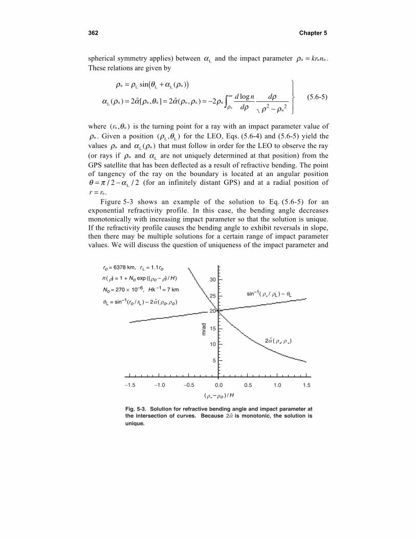
362 Chapter 5
spherical symmetry applies) between αL and the impact parameter ρ* * *= kr n .These relations are given by
ρ ρ θ α ρ
α ρ α ρ θ α ρ ρ ρρ
ρρ ρρ
* *
* * * * * *
*
L L L
L*
sin ( )
( ) ˜[ , ] ˜ ( , )log
= +( )
= = = −−
∞
∫2 2 22 2
d n
d
d (5.6-5)
where ( , )* *r θ is the turning point for a ray with an impact parameter value ofρ* . Given a position ( , )L Lρ θ for the LEO, Eqs. (5.6-4) and (5.6-5) yield thevalues ρ* and α ρL ( )* that must follow in order for the LEO to observe the ray(or rays if ρ* and αL are not uniquely determined at that position) from theGPS satellite that has been deflected as a result of refractive bending. The pointof tangency of the ray on the boundary is located at an angular positionθ π α= −/ /L2 2 (for an infinitely distant GPS) and at a radial position ofr r= *.
Figure 5-3 shows an example of the solution to Eq. (5.6-5) for anexponential refractivity profile. In this case, the bending angle decreasesmonotonically with increasing impact parameter so that the solution is unique.If the refractivity profile causes the bending angle to exhibit reversals in slope,then there may be multiple solutions for a certain range of impact parametervalues. We will discuss the question of uniqueness of the impact parameter and
αFig. 5-3. Solution for refractive bending angle and impact parameter atthe intersection of curves. Because 2 is monotonic, the solution isunique.
α L = sin–1(ro / rL ) – 2 ( o, o )˜θ
ro = 6378 km, r L = 1.1ro
No = 270 × 10–6, Hk –1 = 7 km
n ( ) = 1 + No exp (( o – ) / H )
5
−1.5 1.51.00.5−1.0 −0.5 0.0
10
15
20
25
30
mra
d
( * – o ) / H
sin–1( * / L ) – Lθ
α2 ( *,
* )
ρ ρ ρ
ρ ρ
ρ
ρρ
ρ ρ
ρ
˜
˜

Propagation and Scattering 363
total bending angle for a given LEO position ( , )L Lρ θ in Section 5.12, whichalso addresses multipath and ray caustics.
5.6.1 Defocusing
Because defocusing will arise when we apply the stationary phasetechnique in wave theory, we review it here in somewhat more detail than givenin Appendix A. Defocusing arises because of dispersive refraction. Incomingrays, which were collimated prior to encountering the atmosphere, are dispersedor spread out after entering the atmosphere because of the refractive gradient.To obtain a measure of the defocusing at a given point ( , )r θ , we compute theratio of the signal flux density of an incoming wave prior to encountering theatmosphere with the signal flux density at the point ( , )r θ . This ratio is readilyobtained from Bouguer’s law and by invoking the principle of conservation ofenergy. Let ∆σ be the perpendicular displacement in phase units between tworays (Fig. A-1) in the neighborhood of the point ( , )r θ that results fromchanging the impact parameter by an amount ∆ρ* . Conservation of energyrequires (assuming complete transparency) that the power through a crosssection of width ∆ρ* in the collimated beam prior to atmospheric entry mustequal the power through the cross section of width ∆σ at the point ( , )r θ afteratmospheric entry. Thus, the ratio ζ ρ σ= ∆ ∆* / gives us the defocusing, and itssquare root gives the ratio of the signal amplitudes: the amplitude of the waveat ( , )r θ divided by the amplitude of the collimated wave prior to atmosphericentry.
Upon differentiating Bouguer’s law given in Eq. (5.6-3) with respect to ρ* ,and defining γ θ α= + ˜ , one obtains
Incoming: / :
( / )sin ˜ ( , ) cos ,
Outgoing: / :
( / )sin ˜ ( , ) ˜ ( , ) cos
*
*
*
* * *
π γ π ρ
ρ γ θ α ρ ρ γγ π ρ
ρ γ θ α ρ ρ α ρ ρ ρ γ
> ≥ =
+ ′ + +( )< ≤ =
+ ′ + + −( )
2
0 2
2
∆
∆ ∆ ∆∆
∆ ∆ ∆ ∆
r n n n
r n n n
(5.6-6)
Here
∆ ∆ ∆
∆ ∆
∆ ∆
˜ ( , ) ˜ ˜ ,
˜ ( , ) ˜ ,
( ) , , , ˜
* * *
* * * *
α ρ ρ ∂α ∂ρ ρ ∂α ∂ρ ρα ρ ρ α ρ ρ
ρρ
γ θ α
= +
=
= + ′ ′ = = ′+ ′
= +
d d
k n rn r ndn
drk
dn
d
n
n rn
(5.6-7)
From Eq. (5.6-2), it follows that
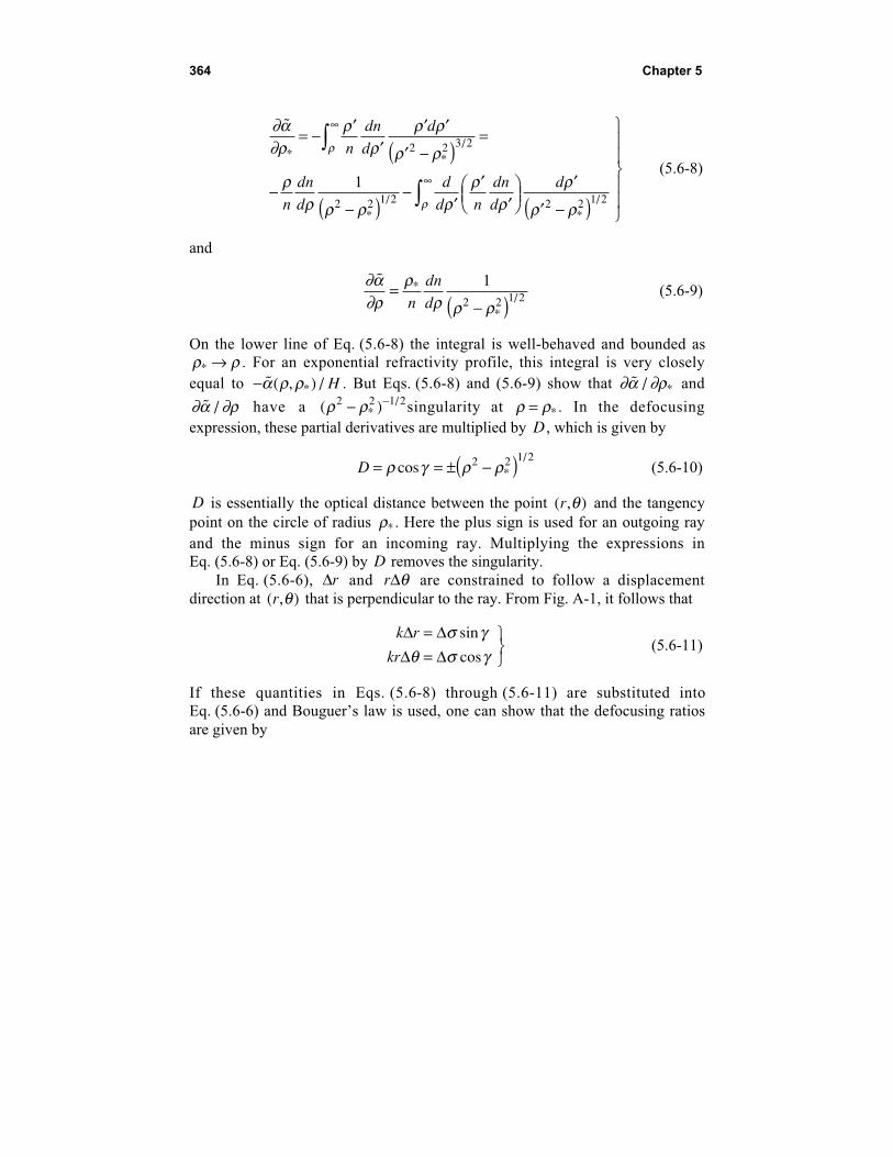
364 Chapter 5
∂α∂ρ
ρρ
ρ ρ
ρ ρ
ρρ ρ ρ ρ
ρρ
ρ
ρ ρ
ρ
ρ
˜
* */
*/
*/
= − ′′
′ ′
′ −( )=
−−( )
−′
′′
′
′ −( )
∞
∞
∫
∫
n
dn
d
d
n
dn
d
d
d n
dn
d
d
2 2 3 2
2 2 1 2 2 2 1 21
(5.6-8)
and
∂α∂ρ
ρρ ρ ρ
˜ *
*/=
−( )n
dn
d
12 2 1 2 (5.6-9)
On the lower line of Eq. (5.6-8) the integral is well-behaved and bounded asρ ρ* → . For an exponential refractivity profile, this integral is very closelyequal to − ˜ ( , ) /*α ρ ρ H . But Eqs. (5.6-8) and (5.6-9) show that ∂α ∂ρ˜ / * and
∂α ∂ρ˜ / have a ( )*/ρ ρ2 2 1 2− − singularity at ρ ρ= * . In the defocusing
expression, these partial derivatives are multiplied by D, which is given by
D = = ± −( )ρ γ ρ ρcos */2 2 1 2
(5.6-10)
D is essentially the optical distance between the point ( , )r θ and the tangencypoint on the circle of radius ρ* . Here the plus sign is used for an outgoing rayand the minus sign for an incoming ray. Multiplying the expressions inEq. (5.6-8) or Eq. (5.6-9) by D removes the singularity.
In Eq. (5.6-6), ∆r and r∆θ are constrained to follow a displacementdirection at ( , )r θ that is perpendicular to the ray. From Fig. A-1, it follows that
k r
kr
∆ ∆∆ ∆
==
σ γθ σ γ
sin
cos(5.6-11)
If these quantities in Eqs. (5.6-8) through (5.6-11) are substituted intoEq. (5.6-6) and Bouguer’s law is used, one can show that the defocusing ratiosare given by

Propagation and Scattering 365
Incoming: :
˜ ( , )
cos
Outgoing: :
˜ ( , ) ˜ ( , )
cos
*
*
*
*
* *
*
*
*
π γ π
σρ
∂α ρ ρ∂ρ
ρ γ
γ π
σρ
α ρ ρρ
∂α ρ ρ∂ρ
ρ γ
> ≥
= −
< ≤
= − −
2
1
02
1 2
nd
d
nd
d
d
d
(5.6-12)
For a point located at the LEO outside of the atmosphere, ˜ ( , )*α ρ ρ → 0 asρ → ∞ , and the outgoing form in Eq. (5.6-12) becomes
d
dD
d
d
σρ
αρ
α α ρ ρ* *
* *
˜
˜ ˜ ( , )
= −
=
1 2(5.6-13)
Here D becomes the distance (in phase units) of the LEO from the Earth’s limbminus ρ α ρ* *L ( ). In practice a GPS satellites is not infinitely distant; its orbitradius is only about 4 Earth radii. To compensate for the wave-front curvatureresulting from this finite distance, it is customary to use the “reduced distance”in Eq. (5.6-13), which is defined in the same way as the “reduced mass” in two-body dynamical systems. This is given by
D D D− − −= +1 1 1L G (5.6-14)
This definition for D follows directly from the Fresnel approximation in thethin phase screen theory (see Section 5.11). This form for D gives a slightlymore accurate measure of defocusing. It also is very useful in thin phase screenanalyses for diffraction and multipath.
For a circular LEO orbit, it follows from Fig. A-1 that ∆ ∆σ θ= D L , where∆θL is the displacement in orbital position of the LEO required to intercept twonearby rays separated in impact parameter by ∆ρ* . In this case of a circularorbit for the LEO, the defocusing equation in Eq. (5.6-13) can be written as
ζ σρ
θρ
αρ
− = = = −1 1 2d
dD
dD
d
d* *
L˜
d *
(5.6-13′)
From Eq. (5.6-2) it follows that
366 Chapter 5
d
d
d
d
d n
d
d
n
d n
d
d
˜ ( , ) ˜ log
˙ ,
* *
* **
*
*
*/ *
*
*
α ρ ρρ
αρ
ρρ ρ ρ
ρρ ρ
ρρ
ρ
ρ ρρ
ρ
ρ
= −
−
= −−( )
>>
∞
∞
∫
∫
2
2 2
2
2 2 2 1 2
1
10
(5.6-15)
For an exponential refractivity profile, d n d H dn d2 2 1/ /ρ ρ= − − , and it followsthat d d H˜ / ˙ ˜ /*α ρ α= − . In this case, the defocusing is related to the deflection2αD at the LEO expressed as the number of scale heights 2 ˜ /αD H thatrefractive bending induces.
At a turning point, γ θ α π= + →˜ / 2 . One could naïvely conclude that thedefocusing factor would reduce to 1 / ( )* * *n r n+ ′ , which is the reciprocal of thederivative of the impact parameter ρ* with respect to the radial coordinate krat the turning point ( , )* *r θ . Equations (5.6-8) and (5.6-10) show that thesingularity in ∂α ρ ρ ∂ρ˜ ( , )* * as ρ ρ→ * yields a finite contribution to thedefocusing ratio at a turning point. From Eqs. (5.6-8) and (5.6-10), Eq. (5.6-12)becomes at a turning point
nd
d n
dn
d
n
n r n**
*
*
*
* * **
σρ
ρρ ρ
= − =+ ′
1 (5.6-16)
thus, confirming our intuition.
5.7 More Asymptotic Forms
We will need asymptotic forms for the functions gl ( )ρ and G[ , ]ρ ν ,defined in Eqs. (5.5-19) and (5.5-20). We also must complete the unfinishedbusiness of fixing that form for gl ( )ρ . The derivation obtained in Section 5.5
based on modified Mie scattering fails when ρ ρ ν< †( ) . We know fromChapter 3 that the principal contributions to the scattering integrals come fromspectral coefficients with wavenumber values in the near vicinity of l = ρ*.Here asymptotic forms that exploit the relatively small value of | | /* *l − ρ ρ butthe large value of ρ* are appropriate. Therefore, we use the asymptotic formsfor the spherical Hankel functions in terms of the Airy functions of the first andsecond kind that have been given in Eq. (5.4-1).
It then follows upon replacing the spherical Hankel functions with theirAiry function asymptotic forms that for gl ( )ρ one obtains the following fromEq. (5.5-19):

Propagation and Scattering 367
g g y
K y y y y yy
K
l ( ) ( ˆ)
Ai [ ˆ] Bi [ ˆ] ˆ Ai[ ˆ] Bi[ ˆ]ˆ
ρ
π νν
→ =
′ + ′( ) − +( ) − +
2 2 2 2 221
5L
(5.7-1)
Here ν = +l 1 2/ . The quantities y and Kν are defined in Eq. (5.4-3) in terms
of ν and ρ . When ν ρ≈ , we can drop the ˆ /y Kν2 term in Eq. (5.7-1) because
of the enormity of ρ* .It follows from Eq. (5.5-20) that the applicable asymptotic form for G[ , ]ρ ν
is given by
Gd n
dg y d y[ , ] ˙
log ˆ , ˆ , ( )†ρ νρ
ρ ζ νρ
ρ ρ νρ
=′
′( ) ′ ′ =′
>∞
∫ (5.7-2)
Here ˆ′y and ′ρ are integration variables, and they are connected through theexpression for y given in Eq. (5.4-3).
If one uses the asymptotic forms applicable to negative arguments for theAiry functions given by Eq. (3.8-7), it follows from Eq. (5.7-1) that
g y y( ˆ) / ˆ ,/
= −( ) + ( ) + ⋅⋅⋅( ) <ρ ν ν ρ2 2 1 2 31 1 16 (5.7-3)
Similarly, from Eq. (5.7-2) it follows for negative arguments that
Gd n
dd[ , ] ˙
log, ρ ν
ρρ ν ρ ν ρ
ρ=
′′ − ′ <
∞
∫ 2 2 (5.7-4)
Even at ν ρ= this asymptotic form for G[ , ]ρ ν is very accurate. The differencebetween the values of G[ , ]ρ ν from Eqs. (5.7-2) and (5.7-4) is roughly0 2 1. / ( )β β− , yielding a relative accuracy in most conditions of a few parts in
105. A super-refractive region (where β ≥ 1 requires special treatment; seeSections 5.8 and 6.4.
From the cumulative bending angle given by Eq. (5.6-2), we have uponintegrating on ρ*
˜ ( , )log
˜ ( , )log
α ρ ν νρ
ρ ρ ρ ν ρ
α ρ ρ ρρ
ρ ν ρ
ν
ρ
ρ
ρ ρ
′ ′ =′
′ − − ′ −[ ] ′
= − ′ ′ ′ −′
′ − ′
∫ ∫
∫ ∫
∞
∞ ∞
dd n
dd
dd n
dd
2 2 2 2
2 2(5.7-5)
From Eqs. (5.7-4) and (5.7-5), it follows that

368 Chapter 5
G d d[ , ] ˙ ˜ ( , ) ˜ ( , ) , ρ ν α ρ ω ω α ω ω ω ν ρν
ρ
ρ= − − <∫ ∫
∞(5.7-6)
We recall that −G[ , ]ρ ν is the phase delay induced by the spherical symmetricatmosphere upon a radial wavelet of wavenumber ν at the radial positionρ = krn. Equation (5.7-6) provides a physical interpretation for these integralsof the bending angle. This is similar in form to the stationary phase conditionthat we found for the thin-screen model in Chapter 2. We note from Eq. (5.7-6)that −2G[ , ]ρ ρ corresponds to the thin-screen phase profile ϕ( )h given inEq. (2.5-1).
Differentiating G[ , ]ρ ν given in Eq. (5.7-2) with respect to ν and using thedefining differential equation for the Airy functions, Ai ˆ Ai Bi ˆ Bi′′ = ′′ =y y, ,[and the near-linear relationship between y and ν given in Eq. (5.4-3)], oneobtains
∂∂ν ρ
∂∂ν
ρ πρ
ρρ ν ρ
G d n
d
dg
dy
yd K
d n
dy y d=
′
′ = −′
′ + ′( ) ′∞ ∞
∫ ∫logˆ
ˆ˙
logAi[ ˆ ] Bi[ ˆ ]2 2 (5.7-7)
For negative arguments of y , we can use the negative asymptotic forms for theAiry functions; Eq. (5.7-7) becomes [alternatively, one can take the partialderivative of Eq. (5.7-4)]
∂∂ν
νρ ρ ν
ρ α ρ ν ν ρρ
G d n
dd˙
log ˜ ( , ), = −′ ′ −
′ = <∞
∫ 12 2
(5.7-8)
Comparing Eqs. (5.6-2) and (5.7-8), we conclude that, for negative values of y ,that is, for ν ρ< , ∂ ρ ν ∂νG[ , ] / may be interpreted as the cumulative bendingangle ˜ ( , )α ρ ν of an incoming ray at the radial position r ( ρ = krn) and withan impact parameter value ν . The accuracy of this correspondence deterioratesonly when ν lies in the immediate vicinity of ρ , that is, near a turning point( , )* *r θ where θ π α ρ ρ* * */ ˜ ( , )= −2 .
Figure 5-4 shows the level of this agreement in the vicinity of a turningpoint for an exponential refractivity profile that decreases with altitude. Itroughly corresponds to the dry air refractivity profile for the Earth near sealevel. Only for spectral numbers in the range ν ρ ν> − ~ 2K does the agreementdeteriorate. Note that ˜ ( , )α ρ ν is not defined for ν ρ> ( y > 0 ) and that
∂α ρ ν ∂ν˜ ( , ) / → ∞ as ν ρ→ − , whereas G[ , ]ρ ν and its derivatives are well-behaved in this neighborhood. However, the form for G[ , ]ρ ν derived inSection 5.5 and its asymptotic form, given in Eqs. (5.7-1) and (5.7-2), changerapidly with increasing ν ρ> because of the behavior of the Airy function of

Propagation and Scattering 369
the second kind. This form fails for ν ρ> . In fact, we show later that g y( ˆ) → 0for increasing y > 0 , and that G[ , ]ρ ν approaches a constant value. The smalldiscrepancies near the turning point result from the deviations of the Airyfunctions from their asymptotic forms for negative arguments, and also fromthe breakdown in accuracy of the spectral coefficients near a turning pointwhen they are derived from Eq. (5.5-21). Figure 5-5 compares ∂ ∂2 2G / ν , adefocusing quantity from wave theory, with the analogous quantity ∂ ∂˜ /α νfrom geometric optics.
That there should be this very close, although not perfect, agreementbetween ray quantities and spectral coefficients from wave theory when thelatter are evaluated at their stationary phase values should not be too surprising.In wave theory, the stationary phase process, which is discussed later, iseffected over spectral number. The value ν ρ= * , which we will show to bevery close to a stationary phase point in wave theory, also provides anequivalent ray in geometric optics between the GPS satellite and the point( , )r θ , and with an impact parameter value of ρ* . The ray path from geometricoptics is in fact a path of stationary phase. Using geometric optics, we may varythe impact parameter over impact parameter space for a ray with constrainedend points. The path has a stationary value of the phase delay when the impactparameter takes on the value ρ ν* = . Any other path with the same end pointsin the neighborhood of the actual ray path would present the observer at ( , )r θwith a phase delay that differed from the observed phase delay by an amountthat has only a second-order dependency on the coordinate and slope deviations
-3 -2 -1
10.2
10.4
9.8
9.6
9.4
1
y
with the cumulative refractive bending angle from geometric
optics, in the vicinity of a turning point.
Fig. 5-4. Comparison of the gradient of the wave theory phase function
( ) ~ , a n n
( ) ~ , a ro n
mra
d
[ ] /,∂ G ∂nro n
[ ] /,∂G ∂n r n ~a
n(r) ( )= 1 +ro - r
H
= 270 ¥
¥
10-6
, H = 7k
ro = kro(1+ No), r = kn(r)r
k = =2p /l 3.32 104
km-1
ro = 6378 km
No
No
exp
-1y n ror
oK )( -=

370 Chapter 5
of the alternate path. This second-order variation would be due to a deviation inthe value of the impact parameter. We will show that, when stationary valuesare assumed by the spectral number in wave theory and by the impactparameter in geometric optics, a close correspondence results.
Consider next the variability of G o[ , ]ρ ν with r for a fixed value of thewavenumber νo . At a point ( , )r θ on the approaching side at large distanceswhere n → 1, we set kr osinθ ν= ; that is, νo becomes the impact parameter forthe ray passing through the point ( , )r θ . Figure 5-6 shows an example ofG o[ , ]ρ ν versus ρ in the vicinity of ρ ν= o . Here an exponential refractivityprofile decreasing with altitude is used, but the altitude range shown in thefigure is very narrow, ~ /7K k
oν , or about 100 meters for the parameter values
shown. This is a small fraction of the refractivity scale height H (7 km)adopted in the figure. On the left side of the figure where y < 0 , that is, whereρ ν> o , the g y( ˆ) function is slowly decreasing with increasing y (decreasingρ ) (see Fig. 5-2), and G o[ , ]ρ ν decreases with increasing y because thegradient of the refractivity is negative. On the right side where y > 0 , g y( ˆ)breaks sharply negative because of the rapid growth of the Airy function of thesecond kind in this region. Therefore, G[ , ]ρ ν , according to the (erroneous)form given in Eq. (5.7-2), rapidly increases with increasing y because therefractivity gradient is negative in the example shown in Fig. 5-6. Therefore,G[ , ]ρ ν has a stationary value at the zero crossing of g y( ˆ) near ρ ν= o . Thecorrect form for G[ , ]ρ ν approaches a constant for increasing y > 0 . This point
( ) /~ ,∂α ∂νρo ν
/~∂α ∂ν
0.5
−3.0 −2.5 −2.0 −1.5 −1.0 −0.5 0.0 0.5 1.0
2.0
µra
d
( ) /,∂ G ∂νρo ν2 2
/∂ G ∂ν2 2
y
Fig. 5-5. Comparison of defocusing quantity from wave
theory with the analogous quantity from geometric optics,
in the vicinity of a turning point.
1.5
1.0

Propagation and Scattering 371
where g y( ˆ) = 0 marks a stationary phase point for al− ( )ρ (with l o= +ν 1 2/ ). It
also is a stationary point for al+ ( )ρ . Later, we will set a al l
+ −= at this point toensure no singularity at the origin from the spherical Hankel function.
For other refractivity profiles, there may be other stationary points forG[ , ]ρ ν , but their occurrence and location are dependent on the functional formof the index of refraction. However, there is always one near ρ ν= o (unlessdn d/ ρ ≡ 0 ), reflecting the “deepest penetration” by the corresponding ray intothe sphere. This region ( y > 0 ) corresponds to refractivity features lying belowthe impact parameter, or the point of closest approach of the associated ray.Such features lying below the point of closest approach are not “felt” by theray. Refractivity features lying near or above the point of closest approach( y ≤ 0 ) are “felt” twice by the ray, incoming and outgoing; these can have aprominent effect on the shape of G[ , ]ρ ν , depending on the actual refractivityprofile.
From the definition of G[ , ]ρ ν in Eq. (5.7-2) and the asymptotic form forg g yl ( ) ( ˆ)ρ → in Eq. (5.7-1), it follows that
∂∂ρ ρ
πρν
G d n
dg y
Kd n
dy y y y y
= −
= − ′ + ′ − +( )( )
log( ˆ)
˙log
Ai [ ˆ] Bi [ ˆ] ˆ Ai[ ˆ] Bi[ ˆ]2 2 2 2 2(5.7-9)
0.5
-4 -2 0 2
1.0
2.0
1.5
2.5
[ ], G r on =r onr
y
†y
y
Fig. 5-6. Variation of with near = obtained from
Eqs. (5.7-1) and (5.7-2). This form is invalid for increasing .
K K
n(r) ( )= 1 +ro - r
- rr r
H
= 270 ¥
¥
10-6
, H = 7k
ro
ro
ro
ro
= kro(1
( ) , r( /2)
+ No), r = kn(r)r
k = =2p /l 3.32 104
km-1
-1 1/3
r no = =
= =
o
G[
rr
] + c
on
sta
nt (ra
d)
,
6378 km,
No
No
exp
> †yy

372 Chapter 5
Upon setting ∂ ∂ρG = 0 , it follows that either g y( ˆ) = 0, or dn d/ ρ = 0 , or bothare zero. Consider first g y( ˆ) = 0 in Eq. (5.7-9). This yields a stationary point fory that is given by
ˆAi ˆ Bi ˆ
Ai ˆ Bi ˆ.†
† †
† †y
y y
y y=
′[ ] + ′[ ][ ] + [ ]
=2 2
2 2 0 44133L (5.7-10)
From the properties of the Airy functions, it can be shown that this value of ˆ†yis unique. We have seen this quantity before in Section 4.6 in regard to turningpoints for waves traveling in a Cartesian-stratified Airy medium.
Upon using Eq. (5.4-3), Eq. (5.7-9) yields a stationary phase point ρ ρ= †
that is a function of νo and which is given by
ρ ν
ρ
ρ
ρ
††
†
†
†
˙ ˆ
/
= −
=
o K y
K2
1 3 (5.7-11)
Thus, | | / / ~† †
†ρ ν ν
ρ− = −
o o y K2 102 6 for νo ~ 108 .
Continuing to the second derivative, ∂ ∂ρ2 2G / , and evaluating it atρ ρ ν= ( )†
o , it follows that
∂∂ρ
πρρ
νρ
2
2
2 2GK
d n
dy y
† †
˙log
Ai ˆ Bi ˆ† †= − [ ] + [ ]( ) (5.7-12)
Setting νo equal to kr n ro o( ) , adopting the Earth’s dry air conditions at sea
level, and using 19 cm for the GPS wavelength, ∂ ∂ρ ρ2 2 610G / | ~†
− rad. It
follows that G will vary from its stationary phase value by the order of 1 radianwhen G | | / ~† †ρ ρ ρ− −10 5 ; in other words, the stationary phase neighborhoodabout ρ ρ= † is very narrow (a few dekameters) when ρ† is so large
(~ 2 108× ).In stationary phase theory (to be discussed in a later section), we will use
∂ ρ ν ∂ν2 2G[ , ] / , which is related to defocusing. A comparison of this secondderivative with ∂α ρ ν ∂ν˜ ( , ) / , also used in geometric optics for defocusing, isshown in Fig. 5-5 for the same conditions given in Fig. 5-4. These also agreeclosely except near a turning point. Accordingly, we expect the accuracy of theamplitude predicted by the osculating parameter technique to degrade fory > −2 . Numerical results verify this threshold. At a turning point, the correct

Propagation and Scattering 373
value for the defocusing in a refracting medium without scattering is given byEq. (5.6-16). At a turning point, the stationary phase value in spectral numberusing the osculating parameter approach is equivalent to y ≈ 0 ; it predicts unitythere for the defocusing.
5.7.1 Equating dG dρ ν ν ν† ,(( ))[ ] // to α ν ν( , ) and d G d2 ρ ν ν ν† , 2(( ))[ ] // tod dα ν ν ν(( )) //,,
We note in Fig. 5-4 at the turning point that the value of ∂ ρ ν ∂νG o[ , ] / at
ν ν ρ ρ= = +† †ˆo K yo
is very close to the value of ˜ ( , )α ρ ρo o . In fact, the actual
numbers for Fig. 5-4 are 10.114 mrad for ˜ ( , )α ρ ρo o and 10.115 mrad for∂ ρ ν ∂νG o[ , ] / . Since ρ ρ ν= †( ) marks a stationary point for G[ , ]ρ ν where∂ ∂ρG / = 0 , it follows that
dG
d
dG
d
G† †
†
( ) ( ), [ , ]νν
ρ ν νν
∂ ρ ν∂ν ρ ρ
≡ [ ] =
=
(5.7-13)
Hence, dG d†( ) /ν ν also will be very close in value to ˜ ( , )α ν ν . We show inAppendix J that
dG
d
d n
d
G G
†
†
( ) ˜ ( , ) O
( ) ( ),†
νν
α ν ν ρρ
ν ρ ν ν
= +
= [ ]
2
2(5.7-14)
Therefore, the difference between dG d†( ) /ν ν and ˜ ( , )α ν ν depends on thecurvature in the refractivity profile. For the thin-atmosphere conditions shownin Fig. 5-4, it can be shown that ρ ρo d n d2 2 310/ mrad( ) ≈ − , which we can
ignore. The difference becomes significant when near-super-refractivityconditions are encountered. See Appendix J.
Similarly, it can be shown that
d G
d
d G
d
G G
d
d
d n
d
2
2
2
2
2
2
2
2
2
2
† †
†
( ) ( ),˙
[ , ] [ , ]
˜ ( , )
O
νν
ρ ν νν
∂ ρ ν∂ρ
∂ ρ ν∂ν
α ν νν ρ
ρ ρ≡ [ ] = − +
= +
=(5.7-15)
For thin-atmosphere conditions, the curvature term here also can be dropped.Equations (5.7-14) and (5.7-15) will play key roles when we apply the

374 Chapter 5
stationary phase technique in wave theory to outgoing waves. Equation (5.7-14)is related to the ray bending angle, and Eq. (5.7-15) is related to defocusing.
Regarding the near-equivalence of dG d[ ( ), ] /†ρ ν ν ν and ˜ ( , )α ν ν , we note aproperty of Bauer’s identity. It is given in cylindrical coordinates inEq. (4.10-9). We can transform θ θ α→ + to obtain
exp cos ( )expi i J illl
l
l
ρ θ α ρ θ α+( )[ ] = +( )[ ]=−∞
=∞
∑ (5.7-16)
Noting that G o[ , ]ρ ν shows up in the exponential term in the spectral seriesrepresentations for the electromagnetic field, its variability with spectralnumber will be related to the angle α above. Thus, we would expect∂ ρ ν ∂νG o[ , ] / to be closely related to an angle, which turns out to be thebending angle.
5.7.2 Fixing the Form for g y( )ˆ when y > 0 by Asymptotic Matching
We have noted the failure of the modified Mie scattering approach tosecure the correct form for g y( ˆ) when ˆ ~y > 0 . Equation (5.7-1) predicts thatg y( ˆ) → ∞ for increasing y > 0 ; in fact, g y( ˆ) should approach zero. We can usethe form for g y( ˆ) obtained from an Airy layer as guidance. In an Airy layerwith a boundary at r r= 0 , the profile for the index of refraction is given by
n n n n r r202
0 02= + ′ −( ), where n0 and ′n are constants. The quadratic term
( ) (( / ))′ −n r r r r02
0 02 is negligible.
In Chapter 4, Section 4.12, we showed that the solutions to the waveequations in a spherical Airy layer are given by the Airy functions. Let U y± ( ˜)be a solution for the scalar field, with the top sign for an outgoing wave and thebottom sign for an incoming wave. When β < 1, from Eq. (4.10-3) andEqs. (4.12-4) through-(4.12-6) we have
U y c y i y± ±= ( )( ˜) Ai[ ˜] Bi[ ˜]m (5.7-17)
where c± are complex constants obtained from matching this Airy functionsolution and its derivative at the boundary r r= 0 with the incoming andoutgoing wave forms applicable on the other side of the boundary. Theargument of the Airy functions is given by

Propagation and Scattering 375
˜ ( )( ˜ ˜ ) ˜
˜
/yK
l
n r
n
kn r
=−
− − + −( )
= − ′
=
1
11
0
2 3 0 0
0
0
0
ρ ββ ρ ρ ρ
β
ρ
(5.7-18)
These forms also apply in a super-refracting medium where β > 1. Also, it iseasily shown that in an Airy layer
ρ ρ
ρ β ρ ρ β ρ ρ ρ
= = + + ′( ) −( ) + ′ −( )= + − −( ) − −( )
krn r k n n r r r kn r r( )
˙ ˜ ( ) ˜ ˜ ˜ ˜ / ˜
0 0 0 0 02
0 0 02
01(5.7-19)
The quadratic term is negligible, and it is dropped. Note that ρ ρ0 0= ˜ . It followsthat the arguments of the Airy functions are related by
ˆ ˙ ˜ /yK
l y= −( ) = −11
0
2 3
ρρ β (5.7-20)
From Eq. (5.7-17), it follows that the phase ψ lA−
of the incoming Airyfunction solution (for β < 1) is given by
ψ lA y
y
−=
+−tanBi[ ˜]Ai[ ˜]
constant1 (5.7-21)
Similarly, by expressing an incoming spherical Hankel function ξ ρl− ( ) in terms
of its Airy function asymptotic form, its phase is given by
ψ lH y
y
−=
+−tanBi[ ˆ]Ai[ ˆ]
constant1 (5.7-22)
The difference ψ ψlA
lH− −
− is the phase accumulation in the l th spectral
coefficient al− ( )ρ for an Airy layer. We denote this phase of the spectral
coefficient by the function ϑ ρ ψ ρ ψ ρl lA
lH− = −
− −( ) ( ) ( ). Taking the derivative
∂ϑ ∂ρl− / , we obtain
∂ϑ∂ρ π ρ
l
K
y
y y
y
y y y
−= −
+−
+
1 1
0
2 2 2 2
˜
Ai[ ˜] Bi[ ˜]
ˆ
Ai[ ˆ] Bi[ ˆ] ˆ(5.7-23)

376 Chapter 5
We note that ∂ϑ ∂ρl− / rapidly approaches zero for increasing y > 0 .
We compare this expression with ∂ ρ ν ∂ρG[ , ] / given in Eq. (5.7-9). Fornegative y , we replace the Airy functions in Eq. (5.7-23) with their asymptoticforms. Then, using Eq. (5.7-20), we obtain
∂ϑ∂ρ
ββ β
ρ ν
ρ
ρ
l
Ky y
y
Ky
n
−→ − − − −( ) =
−− → − ′
−−
1 1
1 1
0
0
3 2 3 2
2 2
( ˜) ( ˆ)ˆ
( )ˆ
/ /
(5.7-24)
whereas, from Eq. (5.7-9), ∂ ρ ν ∂ρG[ , ] / becomes
∂∂ρ ρ ρ β
ρ ννG d n
dg y K
d n
dy
n= − → − − = − ′−
−log( ˆ)
log ˆ21
2 2 2 (5.7-25)
These asymptotic forms are identical for decreasing y < 0 .
Equation (5.7-23) for ∂ϑ ∂ρl− / applies only to an Airy layer, but it is
essentially exact and it applies without restriction on the value of y . On theother hand, ∂ ρ ν ∂ρG[ , ] / obtained from Eq. (5.7-9) is a general form applyingto any physical profile for n r( ) , but it fails for increasing y > 0 . Clearly, wehave a potential match made in heaven. Over the troublesome interval, saybeginning at y > −2 , we can use the form for ∂ϑ ∂ρl
− / given in Eq. (5.7-23).
The range − ≤ ≤2 2y corresponds to a spatial range of 4 6010
k K− ≈ρ m .
Approximating the index of refraction profile by a constant gradient ′n shouldbe fairly accurate in most circumstances, especially since the phase variabilityis rapidly dying out with increasing y > 0 .
If a single Airy layer is not sufficient, then we can form a concatenatedseries of Airy layers near a turning point. Any physical refractivity profile canbe approximated by a series of Airy layers. In this case, β and y would bediscontinuous, according to Eqs. (5.7-18) and (5.7-20), across each boundarybetween Airy layers (see Section 4.7). Applying the continuity conditions to thewave functions and their derivatives across each boundary ties the Airyfunction solutions together for the different layers, which enables one to derivethe phase in any layer. For a given spectral number, whenever one reachesdownward through successive Airy layers to a radial distance ρ ρ ν< †( ) , y
will become positive there, and ∂ϑ ∂ρl− / for that Airy layer rapidly approaches
zero for increasing y > 0 .
Figure 5-7 shows two comparisons of ∂ϑ ∂ρl− / and ∂ ρ ν ∂ρG[ , ] / versus y .
In Fig. 5-7(a), the refractivity profile corresponds to dry air at sea level, but in

Propagation and Scattering 377
Fig. 5-7(b), a rather hefty value of β = 0 9. has been used, hardly thin-atmosphere material.
5.7.3 Behavior of the WKB Solution at a Turning Point
The phase of a wave approaches a constant value as a function of ρ belowa turning point. Its behavior can be quantified by examining the WKB solutions
-3 -2 -1
30
20
mrad/r
ad
mra
d/r
ad
-10
-20
-30
1 2 3
y
y
Fig. 5-7. Gradient of the phase of in an Airy layer: (a) = 0.24 and
(b) = 0.9. is the exact value; - (d log n/d )g( ) is from modified Mie
scattering theory.
b = 0.24
b = 0.9
brb
(a)
(b)
∂Jl-/∂r
∂Jl-/∂r
∂Jl-/∂r
l- ( )a r
yg ( )- d log n
dr
yg ( )- d log n
dr
-3 -2 -1
1.0
0.5
-0.5
-1.0
1 2 3
y
10

378 Chapter 5
to the radial wave equation in Eq. (5.3-5), which are given in Eq. (5.3-10) withf u n u l l ul ( ) ( ( )) /= − +2 2 21 . The incoming and outgoing WKB solutions,
W ul− ( ) and W ul
+ ( ) , can be linearly combined to yield in the fl < 0 regimewhere ρ ν< an exponentially damping solution for decreasing ρ ν< , and alsoan exponentially increasing solution. Using the connection formulas [6]between the WKB solutions for these two regimes, ρ ν< and ρ ν> , we have
f u f u f u
ff du
ff du
ff du
f
l l o l
ll
u
u
ll
u
u
ll
u
u
l
o
o
o
( ) ( ) ( )
exp cos
sinexp
/ /
/
< = >
−( )− −
→
( )−
+
−( )−
←
( )
∫ ∫
∫
0 0 0
1
2
14
4 1
1 4 1 4
1 4 1
π
ϕ π
// cos4 f dulu
u
o∫ +
ϕ
(5.7-26)
where ϕ is an arbitrary phase that is not too close in value to −π / 4 .8 Forf ul = and ϕ π= + / 4 , these are the leading terms of the asymptotic forms for
the Airy functions of the first and second kind.It follows that one solution to the wave equation is exponentially increasing
for decreasing ρ ν< , and the other is exponentially damping to zero. The
asymptotic form of the incoming wave, Ul− , in the ρ ν< regime is a linear
combination of these two exponential solutions. Therefore, the phase of Ul−
must approach a constant value with decreasing ρ ν< . The Airy layer analysis
just discussed shows that the phase of Ul− rapidly approaches a constant;
therefore, ∂ ∂ρG / must rapidly approach zero. Expanding fl in powers of
u uo− and setting n u lo o = leads to f y K y Kl o o= − +ˆ / O[ ˆ / ]ρ ρ
2 2 2 . The
exponential terms in the WKB solutions become exp( ˆ / )/±2 33 2y . For y = 2 ,the ratio of their amplitudes is about 100:1; for y = 3, it is 2000:1.
8 The arrow in each of these two connection formulas indicates the applicable directionof information transfer. For example, continuing the exponentially damping solution inthe f < 0 regime into the f > 0 regime leads to a stable sinusoidal solution in thatregime with “twice” the amplitude and a phase offset of −π / 4 . But the reverse cannotbe guaranteed. Inaccuracy in the numerical computation of the solution to the waveequation starting in the f > 0 regime and integrating downward into the f < 0 regime,even with the phase set equal to −π / 4 exactly, leads inevitably to a numerical solutionthat blows up for decreasing ρ ν< .
Propagation and Scattering 379
5.7.4 Setting G[ , ]ρ ν for ρ ρ ν≤≤ †( )
In the discussions to follow, we have taken a simpler approach in view ofEq. (5.7-6) and also the very close agreement between dG d[ ( ), ] /†ρ ν ν ν and˜ ( , )α ν ν . We let G[ , ]ρ ν run its course based on Eq. (5.7-2) for ρ ν ρ†( ) ≤ < ∞.
I t has a stat ionary value at ρ ρ ν= †( ) . Then we set
G G G[ , ] [ ( ), ] ( )† †ρ ν ρ ν ν ν= = for ρ ρ ν≤ †( ) , a constant value for a given valueof ν . In summary, we modify Eq. (5.7-2) as follows:
G
d n
dg y d
d n
dg y d
[ , ]
log( ˆ ) , ( )
log( ˆ ) , ( )
†
††
ρ νρ
ρ ρ ρ ν
ρρ ρ ρ ν
ρ
ρ
=′
′ ′ ≥
′
′ ′ ≤
∞
∞
∫
∫(5.7-27)
Also, we have
∂ ρ ν∂ρ
ρρ ρ ν
ρ ρ ν
Gd n
dg y[ , ]
log( ˆ ), ( )
, ( )
†
†
=−
′
′ ≥
≤
0
(5.7-28)
This arrangement, which involves some approximation (see Fig. 5-7), alsosimplifies and clarifies the strategy for matching the incoming and outgoingspectral coefficients to eliminate the Hankel function singularity at the origin.We discuss this further in Section 5.8.
5.8 Spectral Representation of an ElectromagneticWave in a Spherical Stratified Medium
We will need to distinguish between an incoming region in the medium andan outgoing region. Figure 5-8 provides an example of the simplest topologyfor these regions. The boundary between these regions is given by the locus ofpoints ( , )* *r θ , which defines the turning point for each ray, where for aspherical symmetric medium E rθ θ( , )* * = 0 . In geometric opticsθ π α ρ ρ* * */ ˜ ( , )= −2 , which is obtained from Eq. (5.6-5). By “incoming” wemean the field at any point where the Poynting vector S E H= ×c( ) / 4π for thewave is such that S r⋅ < 0 . For the simple topology shown by Fig. 5-8, forexample, the incoming region includes any point with a radial position r andan angular position θ that satisfies the condition θ θ π* < < .
When the profile of the refractivity gradient has reversals in polarity, theseregions may not be so simply connected. When a scattering surface is present,

380 Chapter 5
one could obtain both incoming and outgoing waves at the same point.Figure 5-9 sketches a more complicated refractivity profile that also producescoincident incoming and outgoing waves in certain regions.
We first develop the spectral coefficients for the pure refraction case, andwe assume that no scattering surfaces are present in the medium. Scattering ordiffraction occurs where sharp changes in gradient or discontinuities in therefractivity occur. We will deal with those cases later. In particular, we assumethat n r( ) and its derivatives are continuous throughout the medium and that thesimple topology of the kind shown in Fig. 5-8 applies.
Let us evaluate the electric field vector E( , )r θ at a point within therefracting medium in terms of its incoming and outgoing spectral coefficients.We assume that the planar asymptotic boundary condition applies to theapproaching wave and, therefore, al
− is obtained from Eq. (5.5-21). The proper
functional form for al+ is more problematical, and we defer that to later in this
section. From Eqs. (5.3-6), (5.5-2), and (5.5-8), we have the following spectralrepresentation for the in-plane (φ = 0 ) radial and transverse components of theelectric field for the TM wave:
EE
l l a a
EE
a a
ro
l l l l ll
ol l l l l
l
= + ( )
= ′ ′( )
− − + +
=
∞
− − + +
=
∞
∑
∑
21
2
21
1
ρξ ξ θ
ρξ ξ ∂
∂θθθ
( ) P (cos )
P (cos )
+
+
1
1
(5.8-1a)
Because of the enormity of ρ and of l from where essentially all contributionsto these summations originate, we can replace these summations by integrals,which are given by
Fig. 5-8. Schematic of simple incoming and outgoing regions.
Incoming
Outgoing
< s ∑ r > = 0
r*
q*

Propagation and Scattering 381
EE
a a d
EE
a a d
ro
l l l l l
ol l l l l
= ( )
= ′ ′( ) ′
− − + +∞
− − + +∞
∫
∫2
2
22
0
0
ρν ξ ξ θ ν
ρξ ξ θ νθ
+
+
1
1
P (cos )
P (cos )
(5.8-1b)
A similar set holds for the magnetic field. In the limit as n assumes a constantvalue throughout the medium, a a al l l
+ −→ → , and Eq. (5.8-1) reduces to the
collimated form in Eq. (5.5-1) with a i l l lll= + +−1 2 1 1( ) / ( ) , as it must. Also,
using stationary phase arguments, we will show later that in the incomingregion well away from a turning point only the al l
− −( ) ( )ρ ξ ρ term contributes
significantly to the scattering integral; in the outgoing region, only the al l+ +ξ
term contributes. Only for points very near a turning point must we includecontributions from both spherical Hankel functions. This means that, exceptnear a turning point, we may replace the terms al l
± ±ξ / 2 with al l±ψ for
computational purposes, which decays to zero rapidly with increasing l > ρ .
5.8.1 Behavior of ∂ ∂νG /
The spectral representation for the electric field in Eq. (5.8-1b) involvesintegrals over spectral number. To evaluate these integrals using the stationaryphase technique as an aid, we need to find those spectral neighborhoods wherethe phase accumulation of the integrands is stationary. In this regard, we studythe variability of G[ , ]ρ ν with spectral number, ∂ ∂νG / , in terms of therefractivity profile that determines it. We first look at ∂ ∂νG / for two differentrefractivity profiles. Both examples adhere to the thin-atmosphere assumptions.For Case A, n is exponentially distributed so that d drα / is monotonicnegative with altitude; therefore, no multipath or shadow zone situations arise.For this case, ∂ ∂νG / already has been shown in Fig. 5-4. In Case B, n has a
/2
Fig. 5-9. Example of a topology with overlapping incoming and
outgoing regions, from a sharp change in refractivity gradient.
a
To GPS

382 Chapter 5
Gaussian distribution; multipath, shadow zones, and caustics are prominentfeatures for this distribution. These two profiles for the index of refraction aregiven by
n N Ho o= + − −( )[ ]1 exp /ρ ρ (5.8-2a)
n N Hw w w= + − −( )[ ]1 22 2exp /ρ ρ (5.8-2b)
Case B is useful for study of spherical shell structures embedded in an ambientprofile such as that given by Case A. Case B could be used to describe therefractivity profile of a sporadic E-layer in the ionosphere or a marine layer inthe lower troposphere. Case A can be used to describe the Earth’s refractivityprofile for dry air, and the values used for No and H in these examples
correspond roughly to dry air refractivity ( No = × −270 10 6 ) and scale height
( k H− =1 7 km ) at sea level. For computational convenience, we now havewritten these refractivity profiles in terms of ρ ρ= krn( ) , i.e., r is an implicitfunction of ρ .9
For the exponential refraction profile given by Case A, it can be shownusing the thin-atmosphere assumption in the defining path integral for ˜ ( , )α ρ ν ,given in Eq. (5.6-2) [see also Appendix A, Eq. (A-30)], that ˜ ( , )α ρ ν is given by
9 The extraction of n given a value of u kr= through iteration of Eq. (5.8-2) iscumbersome because ρ ρ= un( ) . However, this form for an exponential distribution interms of ρ has some advantages. It results in the very simple form for ˜ ( , )α ρ ν given inEq. (5.8-3), which closely agrees with the numerical integration version for ˜ ( , )α ρ νgiven in Eq. (5.6-2). Provided | / |un n′ < 1, there is a unique relationship between uand ρ . Equation (5.8-3) includes the effects of second-order ray path bending in thepath integral in Eq. (5.6-2). When a positional exponential form is used instead,n u N u u Ho o u( ) exp[ ( ) / ]= + − −1 , the form for ˜ ( , )α νu requires a series in powers of
( / )un n′ to account for higher-order ray path bending. This has been discussed inAppendix A. For a given value of scale height H Hρ = , the version in Eq. (5.8-2a)
gives a smaller radial gradient than the positional exponential version (about 20 percentless for dry air at sea level). This is seen by noting that, for the two versions of theexponential distributions, one obtains the following for dry air at sea level:
H H d n d d n d u d u d n nu / ˙ ( log / log ) ( log / log ) log / log / .ρ ρ ρ ρ= = = − ′ ≈1 1 2
One can adjust the values of the parameters No and H in Eq. (5.8-2a) to attain a close,
but not exact, match with the profile from the positional exponential form; also, thebending-angle profiles from the two versions can be matched rather closely.
For near-super-refractivity situations where un n′ → −/ 1, then the functionalform n( )ρ becomes inconvenient because dn d n un/ /( )ρ = ′ + ′ → ∞1 . But thedefining integral for G[ , ]ρ ν readily allows a change of variable to u .

Propagation and Scattering 383
˜ ( , ) ˙ ( ) erf , α ρ ν ρ πρ ρ νρ
ν ρ= −( ) − −
<n
H H1
21
2
2 2
(5.8-3)
where n( )ρ is given by Eq. (5.8-2a). This expression is very accurate whencompared to the value from the path integral in Eq. (5.6-2). For the decreasingexponential distribution given in Eq. (5.8-2a), the difference is less than1 percent for dry air. Equation (5.8-3) accounts for both the first- and second-order ray path bending effects when the refractivity profile in Eq. (5.8-2a) isused. For the dry air component of the Earth’s atmosphere, the first-orderbending term, 2 1−( ) ′un n/ , contributes less than 10 percent of the total. Thesecond-order ray path bending effect for dry air at sea level amounts to roughly1 percent of the total.
Figure 5-10 shows the variation of ∂ ∂νG / with ν while holding ρ fixedfor Case A. It was obtained from the integral in Eq. (5.7-7). For ν ρ< , we havealready noted from Eqs. (5.6-2) and (5.7-8), and from Fig. 5-4, that∂ ∂ν α ρ νG / ˙ ˜ ( , )= , which holds very accurately for all values of ν nearly up toν ρ= . Numerical integrations of ∂ ∂νG / from Eq. (5.7-7) and ˜ ( , )α ρ ν fromEq. (5.6-2) show microradian-level agreement for both Cases A and B when theinequality ν ρ ρ− < −~ 2K and the thin-atmosphere assumptions are satisfied.
The three curves for ∂ ∂νG / in Fig. 5-10 correspond to three differentradial positions, which are defined, respectively, by ρ ρ− =o H H0 2, / , , andρ ρ= un( ) . The dashed curves in Figs. 5-10 and 5-11 mark the value of ∂ ∂νG /for ν ρ ρ= +* ˆ†
*y K as a function of ρ* , which is a stationary point for G[ , ]*ρ ν .
-1.5 -1.0 -0.5 0.0 1.51.00.5
(~ ,a r* )r*
(~ ,a r* )r*
Fig. 5-10. curves for an exponential refractivity profile. The
dashed curve shows at as varies or, equi-
valently, .
r* ro
+ H /2=r* r
o+ H=
n r*)/H( -
r* ro=
[∂G
∂n,r* ]n
r*
G /∂ ∂nG /∂ ∂n
2
8
6
4
10
14n(r) ( )= 1 +ro - r
H
= 270 ¥
¥
10-6
, H = 7k
ro = kro(1+ No), r = kn(r)r
k = =2p /l 3.32 104
km-1
ro = 6378 km
mra
d
No
No
exp
r*r*= +n †
y K
12

384 Chapter 5
We have shown that at this stationary point dG d G/ / ˙ ˜ ( , )ν ∂ ∂ν α ρ ρ= = withhigh accuracy. Here, ˜ ( , )α ρ ρ is given from either Eq. (5.6-2), or fromEq. (5.8-3) when Case A applies.
Figure 5-11 shows the resulting curves for ∂ ∂νG / , obtained from theintegral in Eq. (5.7-7) when the Gaussian refractivity profile in Eq. (5.8-2b) isused. If this profile also is applied in Eq. (5.6-2) to obtain ˜ ( , )α ρ ρ , a bipolarrefractive bending-angle profile results, which is shown in Appendix E,Fig. E-1, and also as the dashed curve in Fig. 5-11. The bending-angle profilemimics the shape of dn d/ ρ , but it is modified to reflect the geometry of a raytransecting a spherical shell. The intersection of the ∂ ∂νG / curve with the˜ ( , )α ρ ρ curve in Fig. 5-11 also occurs very near the point ν ρ ρ= + ˆ†y K . The
point where the polarity change occurs for ∂ ∂νG / at its initial break pointdepends on the location of the center of the Gaussian distribution relative to ρo.For ρ ρw o< the initial break is negatively directed, but for ρ ρ< w the slope ofn( )ρ becomes negative and ∂ ∂νG / will then break positive. Physically, thisregime where the variability of G[ , ]ρ ν approaches zero, see Eqs. (5.7-26)through-(5.7-28), corresponds to the Gaussian layer being located below thelevel, ρ νo = ; the layer cannot be “sensed” by a ray with an impact parameterν ρ> o . We will show later that there are no stationary phase points in spectralnumber for this regime.
-3
6
-2
1 2 3
Fig. 5-11. curves for a Gaussian refractivity profile for different
locations of its center. The dashed curve is the value of at
(~ ,a r* *)r
[∂G
∂n
,r* ]nn = 1 +
r o2
2
- r-
H
= 0.0001, = 1.6k
r r= D+o
Nw
Nw Hw
Hw
w2
exp( )
*
D = -3/2, - 1, - 1/2, 1/2, 1, 3/2
+ 3/2
mra
d(~ ,a r* )r* or, equivalently, .
wn ro)/H( -
G /∂ ∂nG /∂ ∂n
r* r*= +n †
y K
-1
4
2
-2
+1/2
+ 1
-3/2
- 1
- 1/2
Propagation and Scattering 385
5.8.2 Accuracy of the Osculating Parameter Technique
To check the accuracy of the spectral representation used in this section, asgiven in Eq. (5.8-1), we again use the Airy layer model for a refracting mediumwith spherical stratification. We embed this layer in an otherwise homogeneousmedium. These analytic solutions can be compared with the osculatingparameter and numerical solutions. We let
n n ndn
d
dn
d
kn r kn r n
A A AA
A
A A A A A A
2 2 20
= + −( ) =≤
>
= = = =
˜˜ ,
˜
constant, ˜
, ˜
˜ , ˜ , constant
ρρ ρ
ρρ ρ
ρ ρ
ρ ρ ρ
(5.8-4)
Here ρ ρ= A marks the upper boundary of the Airy layer, and nA is the valueof the index of refraction there. From Sections 4.10 and 4.11, we know that thewave equations for this case are given by
d U
d
n
n
l lU V i
d U
dl
Al l
l2
2
2
21
0˜
˜( )
˜˜ , ˜
˜
˜ρρ ρ
ρ ρρρ
( ) +
− +
( ) = = − ( )
(5.8-5)
U( ˜ )ρ describes the field along the normal to the plane of propagation (they-direction in Fig. 4-10). For a given value of l , U( ˜ )ρ also provides the radialspectral component of the electric field, and V( ˜ )ρ describes the tangentialcomponent parallel to the plane of stratification and in the plane of propagation(the θ -direction in Fig. 4-10).
This model has been discussed in Section 4.12, where a correspondencebetween spherical and Cartesian stratification was established, and also inSection 5.7 to obtain an asymptotic form for G[ , ]ρ ν valid for ν ρ> . There thesolutions to the wave equations in Eq. (5.8-5) are given to a goodapproximation by the Airy functions with their argument y given byEq. (4.12-5). Thus, in the medium described by Eq. (5.8-4) for r rA≤ , we have
˜ ˙ Ai[ ˜],Bi[ ˜] , ˜ ˙ Ai [ ˜],Bi [ ˜] ,
˜ , ˜
˜ ,
˜ ˜ ˜
/˜
/˜
ρ ρ β
ρ βρ
ρ
ββ ρ ρ
ρ
ρ
U y y V i K y y n
kn rn
dn
d
yK
l
l l A A
A AA
AA A
A
A
= = − ′ ′
= = −
= −−
−( ) −( ) −
−1
1
1
11
1 3 1
2 3 −−( )( )
ρA
(5.8-6)

386 Chapter 5
For the region r rA> , the solutions are the spherical Bessel functions of the firstand second kinds, ψ ρ χ ρl l( ˜ ), ( ˜ ) . We note here that nA is a constant in the Airylayer. Hence, − = =β ρ ρ( / ˜ ) ˜ / ( / ) /dn d n dn dr r n .
At the boundary r rA= , we must match these two solution sets for eachinteger value of l to ensure the continuity of the tangential components of theelectromagnetic field across the boundary. We first match the solutions whenthe Ai[ ˜]y solution applies in the region r rA≤ , that is, the solution that vanishesfor decreasing ρ with ρ < l . Upon noting from Eq. (5.8-6) that
∂ ∂ρ β ρ˜ / ˜ //˜y KA A
= − −1 1 3 (with βA < 1), we set
Ai ˜ ˜ ˜
Ai ˜ ˜ ˜˜
/
y c d
K y c d
A l l A l l A
A A l l A l l AA
[ ] = ( ) + ( )− −( ) ′[ ] = ′( ) + ′( )
−
ψ ρ χ ρ
β ψ ρ χ ρρ
1 1 31(5.8-7)
Using the asymptotic forms for both the spherical Bessel functions and the Airyfunction for − >>y 1 and for − >>y 1, we obtain values for the matchingcoefficients that are given by
cK
X X dK
X X
X y X y
lA
l l lA
l l
l A l A
A A
=−
−( ) = −−
−( )
= −( ) + = −( ) +
1 1
23 4
23 4
1 6 1 6
3 2 3 2
βπ
βπ
π πρ ρ
/
˜
/
˜
/ /
cos ˜ ˆ , sin ˜ ˆ ,
˜ ˜ , ˆ ˆ
(5.8-8)
Here y is given in Eq. (5.8-6), and y is given by Eq. (5.4-3). Their ratio ˆ / ˜y y
is equal to | | /1 2 3− βA .Similarly, for a Bi[ ˜]y solution in the region r rA≤ , that is, the solution that
blows up for decreasing ρ with ρ < l , we set
Bi ˜ ˜ ˜
Bi ˜ ˜ ˜/
˜
y e f
Ky e f
A l l A l l A
AA l l A l l A
A
[ ] = ( ) + ( )
−−
′[ ] = ′( ) + ′( )
ψ ρ χ ρ
βψ ρ χ ρ
ρ
1 1 3 (5.8-9)
When the asymptotic forms apply, that is, at a location well away from aturning point, we obtain

Propagation and Scattering 387
eK
X X d
fK
X X c
lA
l l l
lA
l l l
A
A
= −−
−( ) =
= −−
−( ) = −
1
1
1 6
1 6
βπ
βπ
ρ
ρ
/
˜
/
˜
sin ˜ ˆ
cos ˜ ˆ
(5.8-10)
Referring to our discussion in Section 4.6 on incoming and outgoing wavesin a Cartesian Airy layer, it follows in this case that outgoing and incomingwaves at the boundary can be expressed in the form
Ai ˜ Bi ˜y i y c idA A l l l A[ ] [ ] = ( ) ( )±m m ξ ρ (5.8-11)
The top sign applies to an outgoing wave, and the bottom sign to an incomingwave. Also, the complex coefficients c idl lm( ) provide the phase delay (modulo2π ) between the incoming and outgoing waves at the boundary due to therefracting medium below. This phase delay offset remains invariant for r rA>because the medium is taken to be homogeneous for r rA≥ . From Eqs. (5.8-8)and (5.8-10), it follows that the ratio
c id
c idi X Xl l
l ll l
−+
= −( )( )exp ˜ ˆ2 (5.8-12)
provides the round-trip phase delay between the incoming and outgoingwavelets of spectral number l at the boundary r rA= . From Eqs. (5.8-6) and
(5.8-8) and noting again that in the Airy layer ˆ / ˜ | | /y y A= −1 2 3β , it follows that
˜ ˆ ˜ ˆ
ˆ ˙
/ /
//
X X y y
yl
l l A A
A
AA
A A
A
A
A
− = −( ) − −( )( )
= ⋅−
−( ) = ⋅−
−( )
23
23 1
13 1
2
3 2 3 2
3 23 2β
βρ β
βρρ
(5.8-13)
We return to this expression momentarily after discussing the form of G[ , ]ρ νfor this model of the refracting medium.
Now we use the osculating parameter technique in the spectralrepresentation given in Eq. (5.8-1) to describe the wave in the refracting Airymedium where r rA≤ . The basis functions are the spherical Hankel functions
( ), ( )ξ ρ ξ ρl l+ − , where ρ = knr and n now is variable and given by Eq. (5.8-4).
For a given spectral number, the form for the radial term from Eq. (5.8-1) isgiven by

388 Chapter 5
a a C iG iGl l l l l l l− − + + − += − +( )ξ ξ ρ ν ξ ρ ρ ν ξ ρ+ exp( [ , ]) ( ) exp( [ , ]) ( ) (5.8-14)
Here Cl is a spectral number-dependent complex factor that depends onboundary conditions, which we will discuss later in regard to turning points; itis not of interest here.
From Eq. (5.7-2), it follows that G[ , ]ρ ν for an Airy layer is given by
Gn
dn
dy y
Gn
dn
dy y y y
G
AA A
AA A
[ , ] ˙ ( ˆ) ˆ , ( ) ,
[ , ] ˆ ( ˆ) , ˜ , ˆ ,
[ , ] ,
†
/ /
ρ ν πρ
ρ ρ ν ρ ρ
ρ νρ
ρ
ρ ν ρ
=
− ( )( ) < ≤
→
−( ) − −( ) << −
≡ ≥
61
23
11
0
3 2 3 2
Γ Γ
ρρA
(5.8-15)
Here Γ( ˆ) /y 3 is the integral of g y( ˆ) given in Eq. (5.7-1). Γ( ˆ)y has beendiscussed in Section 4.9 with regard to osculating parameters in a Cartesian-stratified medium, and it is given by Eq. (4.9-5). It is shown in Fig. 5-12. Γ( ˆ)yhas only the two roots shown in this figure, and it is monotonic elsewhere.
For a given value of l in both Eqs. (5.8-13) and (5.8-15), what is the valueof y in Eq. (5.8-15), that is, what value for ρ must we use to match the round-trip phase delay −2G[ , ]ρ ν with the asymptotically exact value of this phase
delay 2( ˜ ˆ )X Xl l− , given from Eq. (5.8-13)? Noting that n is variable inEq. (5.8-15), it follows from Eq. (5.8-4) that
-2 -1
-1
-2
-3
-4
-5
-6
1 2
y
yG(
)
Fig. 5-12. Variation of G(y) in the vicinity of a turning point.
Propagation and Scattering 389
11n
dn
dA
A
Aρρ β
β
= −−
(5.8-16)
We see upon comparing Eq. (5.8-15) with Eq. (5.8-13) that y must be zero.However, the negative argument asymptotic forms for the Airy functions do notapply at y = 0 ; instead, we must set Γ( ˆ)y = 0 in Eq. (5.8-15). This is discussed
in Appendix I, Eq. (I-11), with regard to relating dG d[ ( ), ] /†ρ ν ν ν to ˜ ( , )α ν ν .The roots of Γ( ˆ)y occur at ˆ ˙ .y = −0 2 and +0 9. , and Γ( ˆ)y reaches a stationary
value of almost zero at ˆ ˆ†y y= . It is nearly zero there compared to the value of
( ˆ ) /−yA3 2 when − >>yA 1 (see Fig. 5-12). Thus, we set ρ ρ ν ρ= = −† †K y to
force a near alignment of Eq. (5.8-15) with Eq. (5.8-13). The relative error ofthis choice is Γ Γ( ˆ ) / ( ˆ ) .†y yA ≈ 0 001 for this example.
In Section 5.5, Eqs. (5.5-22) through (5.5-25), we discussed the spectralcoefficients al
+ for an outgoing wave in terms of G[ , ]ρ ν . The equation for al+
involved a constant of integration al+[ , ]* *ρ ρ . The question of the appropriate
value of ρ* to use in this constant of integration was left rather moot in that
discussion. Here we set ρ ρ*†= and
a il
l liGl
l+ −[ ] = ++
−( )ρ ρ ρ ν† † †,( )
exp [ , ]1 2 11
(5.8-17)
This provides a rationale for setting ρ ρ ν= †( ) in 2G[ , ]ρ ν for the outgoingwave, at least when well away from a turning point so that yA < 0 . We willreturn later to this question of linking the incoming and outgoing spectralcoefficients.
5.8.3 Numerical Comparisons
Although the close comparison between 2G[ , ]†ρ ν and c id c idl l l l−( ) +( )/at the boundary of the Airy layer is encouraging, we should compare theosculating parameter representation for the wave given in Eq. (5.8-14) with theexact solution obtained from integrating the wave equations in Eq. (5.8-5).Their level of agreement as a turning point is approached is of particularinterest. Figure 5-13(a) shows the solution for Ul ( )ρ , which is the solution tothe wave equations in Eq. (5.8-5), and it also shows the osculating parametersolution from Eq. (5.8-14). They are virtually doppelgangers over the rangeshown for y . In this example, ν ρ= + = =l ko1 2 6400/ , ρA k= 6432 ,
k = −100 1km , ′ = × −n 1 56 10 4. , and no = 1. The solution is closelyapproximated by Ai[ ˜]y . It yields a single-sided bending angle at

390 Chapter 5
ρ ρ* = =o k6400 of 10 mrad, and this medium has a moderate ray pathcurvature index β of about 0.1. The general procedure in Figs. 5-13 through5-16 for comparing these solutions is as follows. For initial conditions, we setU yl ( ) Ai[ ˜ ]† †ρ = , and we also equate their derivatives at this point. Thisgenerates a numerical solution for Ul ( )ρ that exponentially damps to zero fordecreasing ρ in the vicinity of the turning point at ρ νo = (but it blows up forρ ρ<< o because of limited numerical precision). Then at ρ ρ= A , which in theexample shown in Fig. 5-13 corresponds to a y value of about –50, we set
C a al l l l l( ( ) ( ) ( ) ( ))− − + +ρ ξ ρ ρ ξ ρ+ equal to the numerical solution for Ul ( )ρ there,and we also equate their derivatives there. This sets the complex value of Cl inEq. (5.8-14) and gives the osculating parameter solution for decreasing ρ .
-30-40 -20 -10
0.004
0.002
0.006
-0.004
-0.002
-0.006
y
Fig. 5-13. Comparison of from a numerical integration of Eq.
(5.8-5) in an Airy layer with the osculating parameter solution: (a)
wave equation solutions and (b) the difference between the solutions.
-30-40 -20 -10
0.4
0.2
0.6
0.8
-0.4
-0.2
-0.6y
(U )~l r
D =
(a)
(b)
Ul (r) and
Ul (r- )
Cl l(a+l+(r) (r)x + la- -
l(r) (r))x
Cl l(a+l+(r) (r)x + la- -
l(r) (r))x

Propagation and Scattering 391
Figure 5-13(b) shows the difference between Ul ( ˜ )ρ and the osculatingparameter form with the same initial conditions at the boundary r rA= . HereG[ , ]ρ ν is obtained from Eq. (5.5-20), integrated on ρ over the Airy layer fromρA to ρ . In the osculating parameter solution for these two panels, G[ , ]*ρ ρaccumulates about 3 1/2 cycles between rA and r† , where r k n† † †/ ( )= −1ρ ρ .This accumulation of 3 1/2 cycles is required to keep the solutionC a al l l l l( )− − + +ξ ξ+ in Eq. (5.8-14) aligned in phase with the exact solution Ul ( )ρover the entire Airy layer. Better than 1 percent numerical agreement holdsbetween solutions except very near a turning point. As expected, for ˆ ~y > −2the osculating parameter solution begins to deteriorate, but even at y = 0 it stillis moderately accurate for this example; the difference is 0.007. The differentialequations in Eq. (5.8-5) become numerically unstable for y > 0 . Any smallnumerical errors in matching the boundary conditions or in the numericalintegration will magnify greatly in the region y > 0 ; that is, Bi[ ˜]y beginsleaking into the numerical solution. See the discussion of the connectionformula for the WKB solutions in Eq. (5.7-26). Matching boundary conditionscloser to y = 0 , for example at y = −5 , improves the overall agreement, but theosculating parameter solution still deteriorates rapidly for y > 0 . But, thenumerical solution for Ul also deteriorates for y > 0 because of limitedprecision.
The wavenumber k = −100 1 km used in Fig. 3-14 is more than 300 timessmaller than the wavenumbers of the GPS navigation signals. The smaller valueis used here to save computational time and to preserve computationalaccuracy—for given values of rA and r*, the number of cycles in the solutiondepends linearly on k . It is difficult to maintain coherency between solutionsby matching both the solution and its derivative at the same point for highlyoscillatory systems. The runoff error is roughly proportional to k . Small errorsin the computation of Ul and G[ , ]ρ ν inevitably lead to runoff. An alternatematching strategy to reduce runoff is to pick two separate points and matchsolutions there, but not their derivatives.
Figure 5-14 shows another comparison between the numerical andosculating parameter solutions. Here a moderately strong refractivity gradienthas been used, leading to single-sided bending-angle variations of more than30 mrad over a tangency point altitude range of 8 km. Figure 5-14(a) shows theprofile of the refractivity change, and Fig. 5-14(b) shows the resulting bending-angle profile. In the lowest layer, ρ ρdn d/ .= −0 8 , which gives a ray pathcurvature index of β = 4 9/ . But in the middle layer, ρ ρdn d/ .= +0 8 , whichyields β = −4 , a rather extreme negative ray path curvature. Figure 5-14(c)
compares the two solutions, Ul ( )ρ and a al l l l− − + +( ) ( ) ( ) ( )ρ ξ ρ ρ ξ ρ+ . Here the

392 Chapter 5
-0.75
-0.50
-0.25
0.00
0.25
0.50
0.75
1.00
2 4 6 8
Fig. 5-14. Comparison of wave equation solutions in a strong
refracting medium: (a) refractivity profile, (b) bending angle
profile, and (c) wave equation solutions, and(r )Ul+ r x+ rC
l(a
l( )
l( )
+ - r x - ral
( )l
( )).
(r ) and
+ r x+ r + - r x- r
Ul
Cl(a
l( )
l( ) a
l( )
l( ))
r - ro (km)
(c)
-10
20
30
40
50
10
4 6 82
(mra
d)
a
r - ro (km)
(b)
-100
-200
-300
-400
-500
2 4 6 8
¥10
6N
r - ro (km)
(a)

Propagation and Scattering 393
radial distance r , with a range of 8 km and with k = −400 1km , is used for theabscissa instead of y . Per the discussion in Section 5.7 concerningEqs. (5.7-25) and (5.7-26), by forcing the osculating parameter solution tofollow the Airy layer solution for y values greater than ~ −2 , roughly 1/2 km
above the turning point for k = −400 1km (~30 m for GPS wavelengths), onecan greatly improve the solution below the turning point, until the numericalsolution itself begins to fail.
Figure 5-15 compares the wave equation solutions for a severely refractingmedium that includes a super-refracting layer, 1-km thick in the ranger r rd u< < . The refractivity profile is shown in Fig. 5-15(a). Within the super-refracting layer, the ray path curvature index has a value of β = 2 . Above thelayer, β = 0 4. , and below it, β = 0 3. . These refractive gradients lead toenormous swings in the ray path bending angle. Figure 5-15(b) shows theresulting single-sided bending-angle profile versus tangency point radius,including the super-refracting zone r r rc
u< <* . For tangency points within thisrange, no rays can occur when spherical symmetry applies. Figure 5-15(c)shows the variation in impact parameter in the vicinity of this super-refractinglayer. The impact parameter has a negative slope within the layer.Figure 5-15(d) compares the wave equation solutions. In this example, theturning point is well below the critical radius, i.e., r ro
c< . Good agreement
holds except near the turning point. A wavenumber value of k = −1000 1km isused in Figs. 5-15 and 5-16. The wave equation solutions in Fig. 5-15(d) showa slight amplitude bulge and a slight reduction in frequency in the vicinity ofthe super-refracting layer, which is expected. Referring to the WKB solutionconnection formulas in Eq. (5.7-26), the amplitude and frequency factorexpressed in length units is f k y K yl ( ) ˙ ˆ / ˆ kmρ ν= − ≈ − −2 2 246 . When β < 1,∂ ∂ˆ /y r < 0 ; but in a super-refracting medium where β > 1, then ∂ ∂ˆ /y r > 0 . Itfollows that ∂ ∂f rl / > 0 for r rd< ; but within the super-refracting layer,r r rd u< < , ∂ ∂f rl / < 0 . For a turning point below the critical tangency point,
i.e., for ν < kn r rc c( ) , fl ( )ρ remains positive for all r k n r> −1ν / ( ), but itbecomes less positive with increasing r within the super-refracting layer,which is reflected in the figure by the increasing amplitude ( ~ /1 4 fl ) and
decreasing frequency ( ~ fl ) within the layer. Above the layer, ∂ ∂f rl / returns
to positive territory. When ν < kn r rc c( ) , the l th spectral component of thewave effectively powers through the super-refracting layer, as shown inFig. 5-15(d). The corresponding ray, with an impact parameter valueρ ν* ( ) ( )= ≤ =kn r r kn r rc c
u u, also powers through, although it is severely
refracted as ρ* ( )→ kn r rc c from below.

394 Chapter 5
Fig
. 5-1
5.
C
om
pari
so
n o
f w
ave eq
uati
on
so
luti
on
s in
a severe
ly re
fracti
ng
m
ed
ium
w
ith
a su
per-
refr
acti
ng
la
yer:
(a)
refr
acti
vit
y p
rofi
le,
(b)
ben
din
g a
ng
le p
rofi
le,
(c)
imp
act
para
mete
r p
rofi
le,
an
d (
d)
wave e
qu
ati
on
so
luti
on
s;
sp
ectr
al
nu
mb
er
.
2
10
1 023
23
45
67
8
46
8
−0.2
0.2
0.4
−0.4
(d)
(c)
(b)
(a)
Ul(
ρ) a
nd
Cl
r−
r o
r ur d
−r o
r ∗
=kn
(ro)r
o <
kn(r
c)r
cν
r ur d
rc
rc
rc
l(a
+l+
( ρ)
( ρ)
ξ+
la
−− l
( ρ)
( ρ))
ξ
2
−600
−400
−500
−200
−100
−300
−700
46
−r o
r(k
m)
810
−r o
r(k
m)
ρρ −)/k (km) (o ∗
uρ d ρ
50
40
30
20
10 0
2
No R
ays
04
68
r ur d
× N106
()(mrad) r ~α

Propagation and Scattering 395
Fig
. 5-1
6.
Co
mp
ari
so
n o
f w
ave eq
uati
on
so
luti
on
s w
ith
th
e sp
ectr
al
nu
mb
er
locate
d in
th
e su
per-
refr
acti
ng
zo
ne:
(a)
wave
eq
uati
on
so
luti
on
s w
ith
, (
b)
pro
file
fo
r
fo
r (a
), (
c)
wave e
qu
ati
on
so
luti
on
s w
ith
, an
d (
d)
pro
-
file
fo
r f
or
(c).2
46
8
−0.5
0.5
1.0
−1.0
(c)
(d)
(b)
(a)
Ul(
ρ)
r−
r o
kn
(ru)r
u<
<kn
(r c
)r c
νkn
(ru)r
u<
<kn
(r c
)r c
ν
= kn(r
c)r
cν= kn(r
c)r
cν
24
68
−0.5
0.5
1.0
−1.0
r−
r o
1
−8 −10−4−2 −6
23
−r o
r
45
y
y
1
III
V
IVIV
I
II
−8 −10−4−22 −6
23
−r o
r
45
yy
Ul(
ρ)C
ll
(a+
l+( ρ
)( ρ
)ξ
+l
a−
− l( ρ
)( ρ
))ξ
Cl
l(a
+l+
( ρ)
( ρ)
ξ+
la
−− l
( ρ)
( ρ))
ξ

396 Chapter 5
As the ray path tangency point approaches the critical radius r rc* = , the
bending angle approaches a limit, shown in Fig. 5-15(b), and the wave solutionshows a marked transition from an oscillatory form to an exponential form inthe vicinity of the layer. A delicate situation occurs when the turning point issuch that kn r r kn r rc c
d d( ) ( )≤ ≤ν . Here fl ( )ρ reverses sign at kn r r( ) = ν , with
the lower root to the equality lying in the range r r rcu< < , and the upper root at
r ru> . In this case, we have two zones where Ul ( )ρ must be exponential-like:in that region in and above the super-refracting layer where fl < 0 , and belowthe turning point where fl < 0 again. Inasmuch as there are no rays for
tangency points in the range r r rcu< <* , we expect the wave equation
equations to give a damped amplitude for the field.Lastly, Fig. 5-16 shows the case where the spectral number has been
increased (actually, the refractivity profile was lowered in altitude relative to afixed turning point) so that the spectral number lies in the rangekn r r kn r r kn r rc c
o o d d( ) ( ) ( )≤ = ≤ν . This figure shows the wave equationsolutions and the profile for y . Figures 5-16(a) and 5-16(b) are for the case
where ν = =kn r r kn r rc cu u( ) ( ) , the critical impact parameter value marking the
boundaries of the zone corresponding to the altitude range r r rcu< <* , within
which no ray path tangency points may lie. Figures 5-16(c) and 5-16(d) are forthe case where the spectral number lies within the critical rangekn r r kn r ru u d d( ) ( )< <ν , the equivalent of about 150 m in radial distance above
rc for k = −1000 1km . Figures 5-16(a) and 5-16(c) were normalized so that theamplitudes of all of the wave equation solutions in Figs. 5-16(a) and 5-16(c)have the same asymptotic value with increasing r well above the atmosphere.Here the agreement between Ul ( )ρ and the osculating parameter solutionsdegrades significantly in the vicinity and below the super-refracting layerbecause y becomes positive over a limited interval about the upper boundary atr ru= . It also becomes positive again below the turning point. Although the
amplitudes of the two solutions diverge below the layer, their phases remainaligned right down to the turning point.
A super-refracting layer acts like a second turning point when the spectralnumber lies in the critical zone kn r r kn r rc c
d d( ) ( )≤ ≤ν . We note fromEq. (5.7-26) that the slightest hint of a positive value for y in the super-
refractive zone ( − = ≈f k y K yl ˙ ˆ / ˆν 7 ) causes Ul ( )ρ to damp to near-zerobelow the lower critical point where y = 0 . The easiest way to see this is toconsider the reverse sense of propagation. Consider a solution for Ul ( )ρ that isforced to damp to zero below the turning point at ρ ρ= o . With these initialconditions on Ul ( )ρ and its derivative, the solution then is propagated outward.

Propagation and Scattering 397
When the region above the turning point where fl ( )ρ first becomes negative isencountered, the solution becomes exponential-like. This causes the amplitudeof Ul ( )ρ , which still has an Airy function-like character (of the first kind)below this point, to be catapulted to an astronomical magnitude if fl ( )ρremains negative for a sufficient interval.10 But we have normalized theasymptotic values of the outbound amplitudes to correspond to the amplitude ofan incoming wave, which is essentially invariant over the narrow range ofspectral numbers considered here. This forces the amplitude of Ul ( )ρ in theregion below the lower point at which fl ( )ρ = 0 to be greatly diminished whenˆ ˆ
MAXy yu= is positive. In Fig. 5-16(a), ˆ ˙MAXy = 0 , and the amplitude of Ul ( )ρbelow the layer is beginning to attenuate. But in Fig. 5-16(c), ˆ
MAXy is barelypositive, 1.1, and fl ( )ρ is negative only over a 40-m interval about r ru= .Already for these slight intrusions the amplitude of Ul ( )ρ is an order ofmagnitude diminished below the layer. For GPS wavelengths, ∆y = 1
corresponds to ∆r = 14 m and − ≈f yl 70 ˆ . Therefore, the cutoff in amplitudeof Ul ( )ρ below a super-refracting layer for spectral numbers greater than thelimiting value yielding ˆ
MAXy = 0 is extremely sharp.The lower point for r ru< in the super-refracting layer where y = 0 is also
the first point where the bending-angle integral for a hypothetical ray with animpact parameter value of ρ ν* = would become complex, if such a ray were toexist. Here kn r r( ) becomes smaller than ρ* for increasing r above this pointuntil the upper point where y = 0 is reached at r ru< .
A better approximation approach (but not used here) for the osculatingparameter solution to obtain closer alignment with Ul ( )ρ in and below thesuper-refraction zone is to break the spherical medium into regimes. InFig. 5-16(d), these regimes are designated by Roman numerals, and they haveboundaries in the radial coordinate r at the points where y ≈ −2 . In I and IV,the osculating parameter solution applies because y < −2 throughout theseregimes. In each of the tunneling regimes, II, III, and V, the refractivity profile
10 An easy refractivity model with which to see this amplification process is given by
′ = < − × − −n constant km 157 10 6 1 in the super-refracting layer r r rd u
≤ ≤ , and ′ ≡n 0
elsewhere. The wave equation solutions are: below the layer, Ai[ ˆ]y ; within the layer,a y b yAi Bi[ ˜] [ ˜ ]+ ; and above the layer, c y d yAi Bi[ ˆ] [ ˆ]+ . Equating these solutions and
their derivatives across their respective boundaries, at r rd
= and at r ru
= where
ˆ ˆmax
y y= , leads to an explicit evaluation of the coefficients c and d . It can be shown
that the amplitude | | ( ) exp( ( /( )) ˆ / )/ /
max
/c d y2 2 1 2 1 6 3 22 1 2 1 3+ → − −β β β , when ˆmaxy > 0 .
The extreme case ′ → −∞n with ∆n finite is addressed in Chapter 3 (Mie scatteringtheory) and in Section 5.13.

398 Chapter 5
is approximated by an Airy layer, which has a wave equation solution given byEq. (5.8-6). Since y need not be too positive before the solution below the layeris essentially damped to zero, this Airy layer approximation should be valid.The coefficients of these different solutions are tied together by using thecontinuity conditions on the solutions and their derivatives across eachboundary; these boundaries are marked in Fig. 5-16(d). The amplitude of theosculating parameter solution in IV then will damp to zero rapidly below thelayer, which Ul ( )ρ also does, except for spectral numbers in the transition zonewhere ˆ
MAXy ≈ 0 . On the other hand, in region IV below the super-refractionzone, G[ , ]ρ ν contains valid phase information because ˆ ~y < −2 .
In summary, Figs. 5-13 through 5-16 show good agreement between theexact and osculating parameter solutions over almost all regions except those inthe immediate neighborhood of a turning point or in that delicate transition
across the critical spectral number range ν ≈ ( )kn r rc c , below a super-refractinglayer. Here ˆ
MAXy ≈ 0 , but it is not yet positive enough to rapidly damp Ul ( )ρ tozero below the layer. In calculating the electric field from the integrals overspectral number that are given in Eq. (5.8-1b), Section 3.16 shows that theprincipal contribution to these integrals comes from a neighborhood in spectralnumber where the phasor in the integrand is varying the least. This is astationary phase neighborhood, which may or may not be unique, depending onthe refractivity profile. If the field is being evaluated at an incoming point wellaway from a turning point, then a stationary phase neighborhood will not belocated near y = 0 , but rather in negative territory. Therefore, except forincoming positions near a turning point, we expect the accuracy of theosculating parameter technique applied to the spectral integrals in Eq. (5.8-1b)to be adequate. Moreover, near a turning point, one can use the Airy layerapproximation to greatly improve the accuracy there, which is discussed inSection 5.11. The issue of outgoing points remains, and it is discussed later.
5.8.4 Comparison of Phase Delays in an Airy Layer from WaveTheory and Geometric Optics
According to geometric optics, the single-sided phase delay for an initiallycollimated incident ray with an impact parameter ρ ρ* ≤ A is given by
ck kn rdr
n r n r
d n
dd
r
rA Aτρ
ρ ρ ρ
ρ ρ ρ α ρ ρ α ρ ρ
ρ
ρ=
−= − −
+ − + − ( )( )
∫ ∫2
2 2 2 2
2 2
2 2
* *
*
* * * * *
* *
log
˜ ( , ) ˜ ,A A
(5.8-18)
The second equality follows from integrating by parts and using Eq. (5.6-2) forthe bending angle. Using Bouguer’s law, we see that the bottom line simply

Propagation and Scattering 399
equals ρ θ αA Acos sec( ˜ )∆ through second order in ∆ ˜ ˜ ( , )* *α α ρ ρ= − ˜ ( , )*α ρ ρA .Therefore, the extra single-sided phase delay caused by the refractive gradientfor a ray with an impact parameter ρ ρ* ≤ A is given by
ckd n
dd
r r
r
A A
A
A∆τρ
ρ ρ ρ β ρβρ
ρ= − − =
−( )−( )
∫ log
˙*
** *
*
/2 2
3 2
3 1
2(5.8-19)
The approximate expression on the RHS applies to the Airy layer model, and itis accurate when thin-atmosphere conditions apply and r* / λ >> 1 (seeAppendix A). This expression also gives about 3 1/2 cycles for the conditionsshown in Fig. 5-13, and it matches the phase delay expression given inEq. (5.8-13).
Equation (5.8-13), which is an asymptotically exact result for an Airy layer,Eq. (5.8-15), which gives G[ , ]ρ ν from use of the osculating parametertechnique, and Eq. (5.8-19), which is from geometric optics, all essentiallyagree on the phase induced by the refractive gradient on a wave passing throughthe Airy layer. We return to this model in Section 5.11, where calculating thefield at a turning point is discussed.
Equation (5.8-19) provides us with further insight into the character ofG[ , ]ρ ν . When ν ρ*
*= , G[ , ]*ρ ρ provides the extra path delay for a ray withan impact parameter value of ρ* , both from the curvature component of the raythat is induced by the refractive gradient and from the change in wave velocityalong the ray in the medium.
5.8.5 Asymptotic Matching the Spectral Coefficients for Incomingand Outgoing Waves
Let ( , )* *r θ mark a turning point and ρ* * *= kr n be the impact parameterassociated with the ray passing the turning point. We know from Bouguer’s lawfor a spherical symmetric medium that ρ* is a constant when evaluated alongthat ray path.
When the planar asymptotic boundary conditions apply to the approachingwave, then the incoming spectral coefficient al
− ( )ρ is uniquely determinedfrom Eq. (5.5-21). It is independent of the impact parameter ρ* associated with
the point ( , )r θ at which al− ( )ρ is evaluated because the asymptotic boundary
conditions in Eq. (5.5-3) for a planar approaching wave are independent ofimpact parameter. Because the wave front surface is not symmetric about theturning-point boundary (the approaching waves are collimated prior toimpacting the medium; the departing waves are dispersed), the outgoingcoefficient depends on the value of ρ* . For the outgoing wave, it follows from
Eq. (5.5-23) that we can obtain al+[ , ]*ρ ρ if we know the value of al
+[ , ]*ρ ρ .
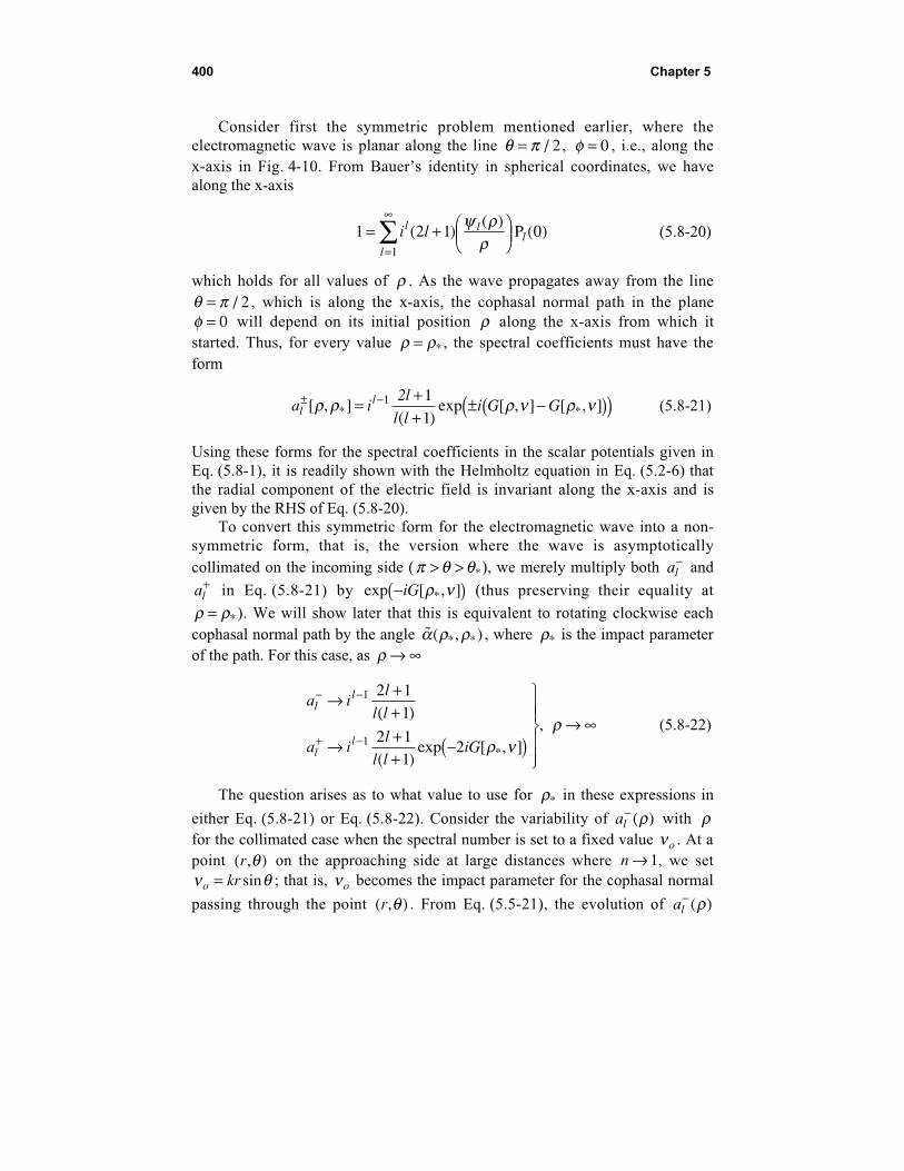
400 Chapter 5
Consider first the symmetric problem mentioned earlier, where theelectromagnetic wave is planar along the line θ π= / 2 , φ = 0 , i.e., along thex-axis in Fig. 4-10. From Bauer’s identity in spherical coordinates, we havealong the x-axis
1 2 1 01
= +
=
∞
∑ i ll ll
l
( )( )
P ( )ψ ρ
ρ(5.8-20)
which holds for all values of ρ . As the wave propagates away from the lineθ π= / 2 , which is along the x-axis, the cophasal normal path in the planeφ = 0 will depend on its initial position ρ along the x-axis from which itstarted. Thus, for every value ρ ρ= * , the spectral coefficients must have theform
a il
l li G Gl
l± −= ++
± −( )( )[ , ]( )
exp [ , ] [ , ]* *ρ ρ ρ ν ρ ν1 11
2(5.8-21)
Using these forms for the spectral coefficients in the scalar potentials given inEq. (5.8-1), it is readily shown with the Helmholtz equation in Eq. (5.2-6) thatthe radial component of the electric field is invariant along the x-axis and isgiven by the RHS of Eq. (5.8-20).
To convert this symmetric form for the electromagnetic wave into a non-symmetric form, that is, the version where the wave is asymptoticallycollimated on the incoming side ( π θ θ> > *), we merely multiply both al
− and
al+ in Eq. (5.8-21) by exp [ , ]*−( )iG ρ ν (thus preserving their equality at
ρ ρ= * ). We will show later that this is equivalent to rotating clockwise eachcophasal normal path by the angle ˜ ( , )* *α ρ ρ , where ρ* is the impact parameterof the path. For this case, as ρ → ∞
a il
l l
a il
l liG
ll
ll
− −
+ −
→ ++
→ ++
−( )
→ ∞
1
1
2 11
2 11
2
( )
( )exp [ , ]
,
*ρ νρ (5.8-22)
The question arises as to what value to use for ρ* in these expressions in
either Eq. (5.8-21) or Eq. (5.8-22). Consider the variability of al− ( )ρ with ρ
for the collimated case when the spectral number is set to a fixed value νo . At apoint ( , )r θ on the approaching side at large distances where n → 1, we setν θo kr= sin ; that is, νo becomes the impact parameter for the cophasal normal
passing through the point ( , )r θ . From Eq. (5.5-21), the evolution of al− ( )ρ

Propagation and Scattering 401
with ν while traveling along this particular ray path can be obtained bystudying the behavior of G[ , ]ρ ν with ν fixed. Figure 5-6 shows an example ofG oρ ν,[ ] versus ρ in the close vicinity of ρ ν= o . G[ , ]ρ ν has a stationary value
at ρ ν ρ= −o y Kˆ† , where ˆ†y is given by Eq. (5.7-10). This point marks a
stationary phase point for al− ( )ρ [and for al
+ ( )ρ ] with respect to ρ . We knowthat the forms for G[ , ]ρ ν given in Eq. (5.5-20) or Eq. (5.7-2) begin to fail forincreasing y > 0 , and that the correct form for G[ , ]ρ ν rapidly assumes aconstant value. Figure 5-7 shows a comparison between the exact phase rate∂ϑ ∂ρl
− / and ∂ ρ ν ∂ρG[ , ] / for an Airy layer.Consistent with the approximation chosen in Eq. (5.7-27) for G[ , ]ρ ν , we
now set a al l+ −= at the point where ˆ ˆ†y y= to ensure no singularity at the origin
from the Hankel functions and to attain a close match with the refractivebending angle. Note that this stationary phase point in ρ space varies with the
value of νo . At this stationary point, ρ ρ ν ν ρ† †
††( )= = − K y , we set
a a il
l liGl l
l+ − −[ ] = ( ) = − [ ]( )ρ ρ ρ ρ ν† †, exp ,† †1 2 11
+
( + )(5.8-23)
This is exactly the same form for al+[ , ]* *ρ ρ that we obtained in Eq. (5.8-17) at
the boundary of an Airy layer to force alignment between the round-trip delayobtained from the osculating parameter technique with the round-trip delayfrom the Airy layer solution. Here G[ , ]ρ ν would include the delay from theAiry layer and from the overlying medium. Of course, our Airy layer can bemade as thin as we please relative to the extent of the overlying medium. Thus,we asymptotically match the incoming and outgoing spectral coefficients.
From Eq. (5.5-23) it follows that al+ ( )ρ is given by
a a i G G
il
l li G G
l l
l
+ +
−
= [ ] − [ ] −( )( )= − [ ] −( )( )
( ) , exp , [ , ]
exp ( ), [ , ]
† †
†
†ρ ρ ρ ρ ν ρ ν
ρ ν ν ρ ν1 2 11
2+
( + )
(5.8-24)
At the LEO, which is located at ( , )L Lr θ and assumed to be outside of therefracting medium where n ≡ 1, the second term in Eq. (5.8-24) is zero; that is,G ρ νL ,[ ] ≡ 0 . It follows that
a il
l li G
y K
ll+ −( ) = − [ ]( )
= −
ρ ρ ν ν
ρ ν ρ
L
† ††
exp ( ),†1 2 11
2+
( + ) (5.8-25)

402 Chapter 5
Thus, − ≡ −2 2G G† †( ) [ ( ), ]ν ρ ν ν is the two-way phase accumulation of the l thspectral coefficient from the stationary point ρ ρ† † †( )= kr n to outside of therefracting medium. It corresponds in geometric optics to the extra phaseaccumulation induced by the refractivity gradient while traveling along a raythat has completely transected the atmosphere and that has an impactparameter value of ν .
We will show later that the value of ν that yields a stationary phase in thewave theory spectral representation in Eq. (5.8-1) is essentially equal to thevalue of the impact parameter for the ray passing through the LEO providedthat the inequality ρ ρ α ρ ρ* * * *| / | ˜ ( , )d n d2 2 << is satisfied. The latter value isgiven from Bouguer’s law by
ν ρ θ α ρ= = = +( )* * * *L L Lsin ( )kr n kr (5.8-26)
where α ρ α ρ ρL ( ) ˜ ( , )* * *= 2 is obtained from Eq. (5.6-5). When multipathsituations occur, this value may not be unique; we will discuss that later. Itfollows that the stationary point for the spectral number in wave theory is givenby
ν ν ρ ρ= = +†* ˆ†
*y K (5.8-27)
A continuing issue for outgoing points concerns the accuracy of theadopted form in Eq. (5.7-27) for G[ , ]ρ ν and, therefore, the accuracy of−2G[ ( ), ]†ρ ν ν in representing the round-trip phase delay. Because of the failure
of the osculating parameter technique for decreasing ρ ρ< † , this adopted formhas some error. But the adopted form for G[ , ]ρ ν does have a stationary value
at ρ ρ= † , and the correct form must rapidly approach a fixed value for ρ ρ< †
(see Fig. 5-7). In addition, we have already noted in Section 5.7 the closecorrespondence between G[ ( ), ]†ρ ν ν and the component of the phase delay inthe eikonal equation induced by the refractivity gradient for a ray with animpact parameter value of ν . Also noted there and in Appendix J is the highaccuracy of the relationship, dG d[ ( ), ] / ˙ ˜ ( , )* * * * * *
†ρ ρ ρ ρ α ρ ρ= , provided that thecurvature in the refractivity profile is moderate. In this section, the closecomparison between −2G[ ( ), ]†ρ ν ν and the exact solution for the round-tripphase delay in an Airy layer has been noted. Moreover, a byproduct of thenumerical solutions presented in Figs. 5-13 through 5-16 (along with the secondnumerical solution for Ul ( )ρ with the boundary conditions generated from
Bi[ ˜ ]†y ) is the exact value of the extra phase delay induced by the refractivitygradient of the medium. G[ ( ), ]†ρ ν ν , based on Eq. (5.7-27) and calculated fromEq. (5.7-2), may be directly compared to this numerical result for the different

Propagation and Scattering 403
refractivity models assumed in these examples. The agreement is generally inthe range of 0.5 to 0.1 percent when the curvature index β is not too close tounity. The computational imprecision in these results also is of the order of0.1 percent. Section 6.5 compares the adopted form for dG d[ ( ), ] /†ρ ν ν ν , akey spectral quantity in the recovery of the refractivity profile from the LEOamplitude and phase observations, with the exact form for an Airy layer. Itgives the error as a function of the ray path curvature index.
An alternative rationale for picking the form given in Eq. (5.8-24) for al+ is
based on probabilistic arguments derived from summing over all possible raypaths. The rationale is similar to the Feynman sum-over-histories technique inquantum electrodynamics to calculate the probability of a quantum event. Onthe incoming side, for an initial planar wave, the probability density distributionof impact parameter values for the rays is a flat curve; each value is equallylikely to occur. Bouguer’s law requires that the flat distribution be preservedafter atmospheric encounter. Therefore, the values of ρ* at a turning point areuniformly distributed. If we set the outgoing spectral coefficient to be thespatial average over all possible impact parameter values to be used inEq. (5.8-22), we end up with an averaging integral to evaluate. The stationaryphase value of this integral yields ρ ρ ν*
†( )= . Therefore, the stationary value of
G[ , ]ρ ν at ρ ρ ν= †( ) should be adopted in Eq. (5.8-22).
5.9 Interpreting Wave Theory in a Refracting MediumUsing the Stationary Phase Technique
We now return to the wave theory spectral representation in Eqs. (5.8-1a)and (5.8-1b) for the electric field at a point ( , )r θ in the refracting medium.Before presenting numerical examples using this spectral representation, weapply stationary phase concepts to aid in the interpretation of those numericalresults to compare with geometric optics. We follow Chapter 3 closely here; inparticular, we refer to the material in Sections 3.10 through 3.13. The integralsin Eq. (5.8-1b) are characterized by a slowly varying factor multiplied by thesum of four phasors that are rapidly oscillating over most of the spectralnumber space. The main contributions to these integrals come fromneighborhoods where any one of these phasors is varying the least. Our tasknow is to use the stationary phase technique on these integrals to identify thepossible stationary phase neighborhoods for each phasor and to calculate thevalues for Er and Eθ at a given point ( , )r θ .
5.9.1 Geometric Interpretation of the Phasors
We rewrite the asymptotic forms for the Hankel and Legendre functions inEq. (5.8-1) in a phasor form that provides a useful geometric interpretation.
404 Chapter 5
Except for a point ( , )r θ located very near a turning point, we will show that thestationary phase neighborhoods in ν space are sufficiently below the valueρ ρ= krn( ) that the negative argument asymptotic forms for the Airy functionsgiven in Eq. (3.8-7) can be used. In this case, from Eqs. (3.10-1) through(3.10-4), the spherical Hankel functions can be rewritten as
ξ ρ ρ ν θ π π
ξ ρρ
ν θ π π
νν ν
νν ν
l
l
Di D
Di D
±
±
± + −( ) −( )( )′
± + −( ) −( )( )
( ) ~ exp / /
( ) ~ exp / /
/
/
1 2
1 2
2 4
2 4
(5.9-1)
where
D krnν νρ ν θ νρ
ρ ρ ν ρ= − =
= <−2 2 1, sin , ( ), (5.9-2)
Similarly, from Eq. (3.10-5), the asymptotic form for the Legendre polynomialP (cos )l
1 θ is given by
P (cos ) ~sin
exp expll
i i1
2 4 4θ
π θνθ π νθ π− +
+ − +
(5.9-3)
The geometric interpretation of θν as the central angle to the point ρ θν,( )and with Dν as its tangential distance in phase units from a spherical causticsurface of radius ν has been given in Chapter 3, Eqs. (3.11-1) and (3.11-2), andin Figs. 3-14 and 3-15. Those figures are applicable to an outgoing wave, butthe concepts are the same, whether incoming or outgoing. Figure 3-14 showsthe geometric relationships given by Eq. (5.9-2). Two rays, originallycollimated from the GPS direction, reach the point L located at ( , )ρ θ . Thedirect path is a straight path to the tangential point P1 and then straight on to thepoint L. Along the retrograde path via P2 , the ray arrives tangentially at P2 ,travels along the arc P P2 2′ , and then departs tangentially from ′P2 going straighton to the point L. We note that, when it is assumed that the stationary phasevalue ν* lies in the range 0 < <ν ρ* , it follows that 0 2< <θ πν * / . As νincreases through its range of values in the spectral integrals in Eq. (5.8-1b), theradius of this caustic sphere expands, and its center descends.
The four phasors appearing in the integrals in Eq. (5.8-1b) result from theproduct of the spherical Hankel and Legendre functions in Eqs. (5.9-1) and(5.9-3) times the incoming and outgoing spectral coefficients given in

Propagation and Scattering 405
Eqs. (5.5-21) and (5.8-24), respectively. To further interpret these phasorsgeometrically, we let
outgoing:
incoming:
θ θ θθ π θ θ
ν
ν
= +
= − +( )
∆
∆v
v (5.9-4)
Because the stationary neighborhoods for ν will be close to ν ρ θ α* sin )= +( ,we would expect ∆θν to be small in these neighborhoods. Figure 3-15 providesa geometric interpretation of ∆θν in terms of the extra phase ν θν∆ along theθ = 0 direction that results from the offset θ θν− for an outgoing wave (andθ π θν− −( ) for an incoming wave).
5.9.2 Stationary Phase Conditions
We now insert the asymptotic forms in Eqs. (5.9-1) through-(5.9-3) intoEq. (5.8-1b), and we substitute the forms for the spectral coefficients al
− and
al+ given by Eqs. (5.5-21) and (5.8-24), respectively. After some manipulation
of Eq. (5.8-1b), the spectral representation for E rr ( , )θ and E rθ θ( , ) becomes
E
Ee e e e d
E
Ee e e
r
o i i i i
o i i i
=
+ + +( )
=
+ +
∞ + + + − − + − −
∞ + + + − − +
∫
∫
2
2 2
1
2
0
0
1
2
πρ θθθ
ν
πρ θθ
ν
ν
θ
ν
sin
sin
cos
sin
sin 2
3( , ) ( , ) ( , ) ( , )
( , ) ( , ) ( , )
Ψ Ψ Ψ Ψ
Ψ Ψ Ψ ++( )
− −e diΨ( , ) ν
(5.9-5)
where the four phases are given by
Ψ
Ψ
Ψ
Ψ
( , ) [ , ] ,
( , ) [ , ] ,
( , ) [ , ]
( , )
†
†
+ + = + +( ) + + − [ ]
+ − = + −( ) − + − [ ]
− + = − − − −( ) + −
− − = − −
D G G
D G G
D G
D
ν ν
ν ν
ν ν
ν ν
ν θ θ π ρ ν ρ ν
ν θ θ π ρ ν ρ ν
ν θ θ π π ρ ν
ν θ
42
42
34
++ −( ) + −
θ π π ρ ν
4G[ , ]
(5.9-6)

406 Chapter 5
Here (±,±) designates use of certain combinations of spherical Hankel functionsand spherical harmonic asymptotic functions. For example in (+, –) the plussign in the first argument designates use of the spherical Hankel function of thefirst kind ξl
+ , and the minus sign in the second argument designates use of thenegative exponential term in the asymptotic form for the Legendre polynomial.In the integrals in Eq. (5.9-5), θν varies slowly with ν , but the phasor termsare rapidly varying except at stationary phase points. The principal contributionto these integrals comes from neighborhoods about stationary phase points. Inthe stationary phase technique, the phase of each phasor is expanded in a Taylorseries through second degree about possible stationary phase values of ν . Thus,the first-degree term is zero, and the Taylor series contains only a zeroth-degreeterm and a quadratic term. Upon evaluating the slowly varying terms at astationary phase point, the integral reduces to a Fresnel integral.
To see if a stationary phase point exists for the four phasors given inEq. (5.9-6), we substitute Eq. (5.9-4) into Eq. (5.9-6) to obtain
Ψ ∆
Ψ ∆
Ψ ∆
Ψ
( , ) [ , ] ,
( , ) [ , ] ,
( , ) [ , ]
( , )
†
†
+ + = + +( ) + + − [ ]
+ − = − − + − [ ]
− + = − − − −( ) + −
− − = −
D G G
D G G
D G
D
ν ν ν
ν ν
ν ν ν
ν
ν θ θ π ρ ν ρ ν
ν θ π ρ ν ρ ν
ν θ π θ π ρ ν
24
2
42
2 234
++ + −
ν θ π ρ νν∆
4G[ , ]
(5.9-6′)
Comparing the terms in Eq. (5.9-6′) with Fig. 3-14, we conclude that ( , )+ + isassociated with an outgoing wave from the far side of the scatteringsphere—that is, it is associated with the retrograde path; ( , )− − is associatedwith the incoming wave on the near side, and so on. We can eliminate byinspection the phase terms Ψ( , )+ + and Ψ( , )− + , because these are associatedwith waves that travel around the far side of the sphere in Fig. 3-14 viapoint P2 . They will provide negligible contributions to the spectral integrals forthe electric field when ro / λ is large and the point L is located well into thefirst or second quadrants in θ . The term 2νθν in their arguments results in veryhigh rates of phase accumulation for essentially all values of ν .
5.9.3 Stationarity of Ψ( , )± ±
Returning to Eq. (5.9-6), we take the partial derivative of the phase Ψ( , )± ±with respect to ν in each of these four phasor combinations that appear inEq. (5.9-6) and attempt to set the resultant equal to zero. We conclude

Propagation and Scattering 407
(remembering that 0 2< ≤θ πν / and that 0 < <θ π ) the following with regardto the possibility of achieving a stationary value for each of these phases:
∂ ∂νΨ( , ) / :+ + = 0
no, if θ ∂ ρ ν ρ ν ∂ν> [ ] −( )2G G*†, [ , ] / ,
∂ ∂νΨ( , ) / :+ − = 0
yes, if θ π ∂ ρ ν ρ ν ∂ν< − [ ] −( )/ , [ , ] /*†2 2G G ,
∂ ∂νΨ( , ) / :− + = 0
no, if θ ≥ 0
∂ ∂νΨ( , ) / :− − = 0
yes, if θ π ∂ ρ ν ∂ν> − [ ]/ , /*†2 G .
As already mentioned, for an occultation from a LEO, we can effectively ruleout the ( , )+ + and ( , )− + combinations. These are contributions to the integralsin Eq. (5.9-5) that originate from the far side of the sphere (Fig. 3-14). They arenegligible when θ lies well into the upper quadrants and when the ratio ro / λis very large, both of which are assumed here. The combination ( , )+ −corresponds to an outgoing wave on the near side of the sphere where thespherical Hankel function ξ ρl
+ ( ) is used; the combination ( , )− − corresponds to
an incoming wave on the near side where ξ ρl− ( ) applies.
5.9.4 Plane Waves
As an illustrative case, consider the stationary phase possibilities for aplanar wave in a homogeneous medium. Here n' ≡ 0 and, therefore,G[ , ]ρ ν ≡ 0 . An appropriate spectral representation for this case is given fromBauer’s identity (Section 5.3) in spherical coordinates:
exp cos ( )( )
P (cos )i i ll ll
jρ θ ψ ρ
ρθ( ) = +∑
=
∞2 1
0(5.9-7)
Here, expressing ill lψ P in terms of phasors (with ψ ξ ξl l l= ++ −( ) / 2 ) leads to
the same combinations Ψ( , )± ± given in Eq. (5.9-6) but with G[ , ]ρ ν ≡ 0 .Attempting to set ∂ ∂νΨ( , ) /± ± = 0 for the four possible sign combinations inthe region 0 < <θ π produces the following conditions on θν :

408 Chapter 5
( , ): ; impossible
( , ): ; possible if 0
( , ): ; impossible
( , ): ; possible if
+ + = −+ − =− + = +− − = − >
θ θθ θ θ πθ θ πθ π θ π θ π
ν
ν
ν
ν
< < / 2
> / 2
It follows that the ( , )+ − case corresponds to a departing planar wave and thatthe ( , )− − case corresponds to an approaching wave. In either case, a stationary
value for Ψ( , )± − is achieved when the spectral number ν ν ρ ρ θ= = =** sin
(see Eq. 5.9-6 with G[ , ]ρ ν ≡ 0 ). For this value, D Dν ρ ρ θ**
| | | cos |= = . The
second derivative of Ψ( , )± − is ∂ ∂ν ν2 2 1Ψ / *= ± −D .
We can evaluate the summation in Bauer’s identity using the stationaryphase technique. Expanding Ψ( , )± − in a Taylor series about the stationary
phase point ν ρ**= through the quadratic term yields
Ψ( , ) ˙ ,
sin , cos
*
*
*
*
**
± − = ± −( )
= = =
DD
D
νν
ν
ν ν π
ν ρ ρ θ ρ θ
12 4
2m
(5.9-8)
Replacing the summation in Bauer’s identity by an integral and usingEq. (5.9-8), we obtain
i l D i d
iDiD i
Dd iD
l ll
j( ) P (cos ) ˙ exp ( , )
˙ exp exp( )
exp
/
*
*
*
*
*
2 11
2
12 2
0
1 2
0
2
0
+∑ = ± ± −( )
= ± ±( ) ± −
= ±( )
=
∞ −∞
∞
∫
∫
ψρ
θπ
ν
πν ρ ν
ν
νν
νν
Ψ
(5.9-9)
By a change of variable π ν ρ νs D2 2= −( ) /* * , the integral in Eq. (5.9-9) is
transformed into a complex Fresnel integral. Since ρ* >> 1, this is essentially a
complete Fresnel integral equal to ( )*/±2 1 2π νiD . Thus, Eq. (5.9-9) reduces to
exp( ) exp( )**
± =iD iDν ρ , which equals the left side of Bauer’s identity.
Note again that 2ψ ξ ξl l l= ++ − . However, ξl− appears in Ψ( , )− − , and ξl
+
appears in Ψ( , )+ − . Therefore, only ξl− contributes to the spectral sum in
Eq. (5.9-9) for a position well within the incoming region, i.e., for an incomingwave. Only ξl
+ contributes for an outgoing wave. This is consistent with the
asymptotic forms that ξl+ and ξl
− assume when ρ ν>> . Here

Propagation and Scattering 409
ξ ρ ρ ρlli i± +→ ±/ ( ) exp( ) /m 1 . Thus, ξ ρl
+ / corresponds to an outgoing
spherical wave, and ξ ρl− / corresponds to an incoming spherical wave.
5.9.5 The Electric Field for an Incoming Wave
We now evaluate the integrals in Eq. (5.9-5) for the electric field vectorusing the stationary phase technique. We first assume that the point ( , )r θ is inthe incoming region well away from a turning point, so that the negativeargument asymptotic forms for the Airy functions apply. In an incoming region,π θ π α ρ ρ> > −/ ˜ ( , )* *2 . If we set as a criterion for “well away” that the point( , )r θ must be such that y < −2 at its stationary phase point, then by applyingBouguer’s law in Eq. (5.6-3), one can show that a suitable criterion isθ π α ρ ρ ρ> − +/ ˜ ( , ) /* * *
2 2 K . For GPS signals in the Earth’s atmosphere,
2 3/ mrad.*
Kρ ≈ In an incoming region well away from a turning point, only
the phase ( ) ( , )i Ψ Ψ= − − contributes significantly to the spectral integrals.We denote the field in an incoming region by (i) E( , )ρ θ , and we
let ( ) ( , )i Ψ Ψ= − − . Thus, ( )i Ψ is the spectral density function for the phasedelay at the point ( , )ρ θ for an incoming wave. It follows from Eqs. (5.9-5) and(5.9-6) for ρ ρ> * that
( )/
( )
( )/
( )
( , )sin
sin
cosexp ( , , ) ,
( , )sin
sin cos exp ( , , )
ir
o i
i o i
EE
i d
EE
i d
ρ θπρ θ
θθ
ρ θ ν ν
ρ θπρ θ
θ θ ρ θ ν ν
ν
ν
θ ν ν
=
( )
= ( ) ( )
∞
∞
∫
∫
2
2
3
0
1 2
0
1 2
Ψ
Ψ
(5.9-10)
To evaluate these integrals using the stationary phase technique, we expand( )i Ψ in a Taylor’s series through second order in spectral number about itsstationary phase value. Using Eqs. (5.9-2) and (5.9-6), ∂ ∂ν( ) /i Ψ becomes
∂∂ν
θ θ π ∂∂νν
( )i GΨ( ) = − + − +
= 0 (5.9-11)
and the second derivative becomes
∂∂ν
∂∂νν
2
2
2
21( )i
D
GΨ( ) = − − (5.9-12)

410 Chapter 5
Let ν* be a spectral number value that provides a stationary phase; that is, itsatisfies the stationarity condition in Eq. (5.9-11). Then from Eqs. (5.9-2) and(5.9-11), one obtains
θ π θ ∂ ρ ν∂ν
ν ρ θ
νν ν
ν
**
*
[ , ]
sin*
= − −
=
=
G
(5.9-13)
We define δ ρ θ ν( , , ) by
θ π θ δ
δ π θ νρ
ρ ρ
ν = − −
= − −
=
−sin
( )
1
krn
(5.9-14)
where for a thin atmosphere δ δ ρ θ ν* *( , , )= generally will be a small quantity.
When ν assumes a value so that δ ∂ ∂ν* /= G , Eq. (5.9-14) shows that we havea stationary phase point. In our discussion in Section 3.12 on stationary phaseprocesses in Mie scattering theory, we noted that δ * should be very close invalue to the refractive bending angle. Here δ * should be close in value to thecumulative bending angle ˜ ( , )*α ρ ρ for a ray passing through the point ( , )ρ θwith an impact parameter value of ρ* . Here ρ ρ θ α ρ ρ* *sin ˜ ( , )= +[ ]. FromEq. (5.7-8), it follows that ∂ ρ ν ∂ν α ρ νG[ , ] / ˜ ( , )= to high accuracy provided
that ν ρ ν< − ~ 2K (see Fig. 5-4). The differences between δ * and ˜ ( , )*α ρ ρ and
between ν* and ρ* can be obtained by expanding Eq. (5.9-14) in a powerseries for G[ , ]ρ ν about the point ν where ∂ ∂ν αG / ˜= , exactly. One obtains
ν ρ δ α ρ θ α
δ α ν ν ∂ ρ ν∂ν ν ν
**
*
* *
˙ ˜ cos( ˜ )
˜ ˙ ˜ [ , ]*
− = −( ) +
− = −( )
=
2
2G (5.9-15)
We expect that ν will be close to ρ* . Upon setting ∂ ∂ν ∂α ∂ρ2 2G / ˜ / *= , itfollows that
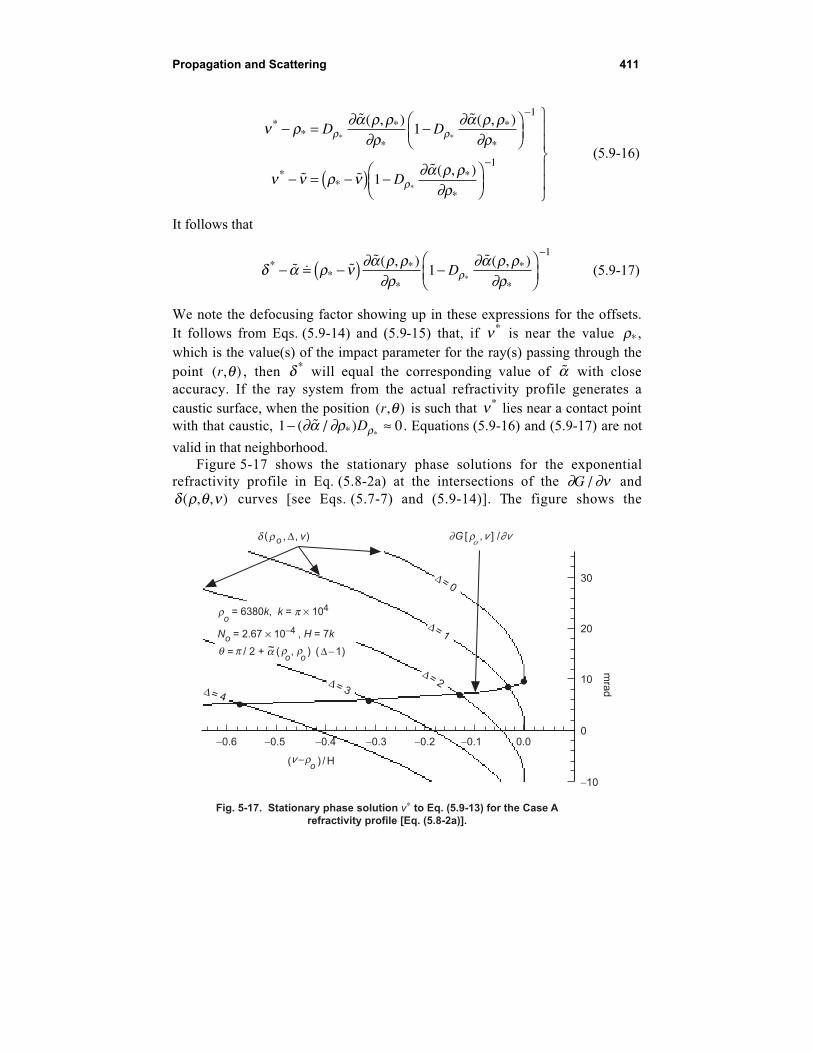
Propagation and Scattering 411
ν ρ ∂α ρ ρ∂ρ
∂α ρ ρ∂ρ
ν ν ρ ν ∂α ρ ρ∂ρ
ρ ρ
ρ
**
*
*
*
*
**
*
*
* *
*
˜ ( , ) ˜ ( , )
˜ ˜˜ ( , )
− = −
− = −( ) −
−
−
D D
D
1
1
1
1(5.9-16)
It follows that
δ α ρ ν ∂α ρ ρ∂ρ
∂α ρ ρ∂ρρ
**
*
*
*
*
˜ ˙ ˜˜ ( , ) ˜ ( , )
*− = −( ) −
−
11
D (5.9-17)
We note the defocusing factor showing up in these expressions for the offsets.It follows from Eqs. (5.9-14) and (5.9-15) that, if ν* is near the value ρ* ,which is the value(s) of the impact parameter for the ray(s) passing through thepoint ( , )r θ , then δ * will equal the corresponding value of α with closeaccuracy. If the ray system from the actual refractivity profile generates acaustic surface, when the position ( , )r θ is such that ν* lies near a contact pointwith that caustic, 1 0− ≈( ˜ / )* *
∂α ∂ρ ρD . Equations (5.9-16) and (5.9-17) are not
valid in that neighborhood.Figure 5-17 shows the stationary phase solutions for the exponential
refractivity profile in Eq. (5.8-2a) at the intersections of the ∂ ∂νG / andδ ρ θ ν( , , ) curves [see Eqs. (5.7-7) and (5.9-14)]. The figure shows the
Fig. 5-17. Stationary phase solution v* to Eq. (5.9-13) for the Case A
refractivity profile [Eq. (5.8-2a)].
mra
d
∂ r v ∂vGo
[ ] /,d r v, ),o D(
D = 0
D = 1
D = 2D = 3D = 4
ov - r( ) / H
pro = 6380k, k = ¥ 104
No = 2.67 ¥ 10-4 , H = 7k
q a D - 1)/ 2 + p ro
ro
( ) (~ ,
-0.6 -0.5 -0.4 -0.3 -0.2 -0.1 0.0
10
0
-10
20
30
=

412 Chapter 5
stationary phase solution for four position points ( , )r θ , all at the same radialdistance ro and with θ increasing from the turning point atθ θ π α ρ ρ= = − ( )* / ˜ ,2 o o in four equally spaced increments up toθ π α ρ ρ= + ( )/ ˜ ,2 3 o o . Even at θ π= / 2 , which is very close to the turning
point and where one might worry that either (1) the asymptotic form at negativearguments for the Airy functions might break down or (2) the approximationsfor the spectral coefficients given in Eq. (5.5-21) for al
− and Eq. (5.8-24) for al+
might fail, the agreement is close. At θ π= / 2 , the intersection point yields astationary phase value that corresponds to an Airy function argument ofˆ*y ≈ −20 . This value for ˆ*y also is corroborated by evaluating Kρ ρ ρ− −1( )*
from Bouguer’s law in Eq. (5.6-3). This justifies our use of the negativeargument asymptotic forms for the Airy functions in the expressions forΨ( , )− − in Eq. (5.9-1) when θ is at least π / 2 or greater. The intersectionpoint for θ π= / 2 in Fig. 5-17 yields a value for ∂ ∂νG / of 8.056 mrad, whichdiffers by only ~ rad5 µ from the value for ˜ , *α ρ ρo( ), ρ ρ* cos= o ∆ , predicted
by ray theory in Eq. (5.6-2). A lower bound on θ already has been establishedfrom Bouguer’s law, where we set ˆ*y = −2 ; this gave θ π α ρ ρ ε≥ − ( ) +/ ˜ ,2 o o ,
ε α= √ ≈−2 31Kuo˜ / . Thus, except for a very narrow range of θ values near the
turning point, the stationary phase point ν* should be very close to ρ* whenthe curvature in the refractivity is relatively slight, i.e., when K kH
oρ / ( ) is
small. K kHoρ / ( ) essentially is the ratio of the Airy function transition scale (a
change in ρ and/or ν corresponding to ∆y = 1) to the refractivity scale height(in phase units), which for the example shown in Fig. 5-17 is about 0.002.
Even at the turning point at θ θ π α ρ ρ= = − ( )* / ˜ ,2 o o , the intersection point
in Fig. 5-17 (where y ≅ 0 in this case) yields a value δ ρ θ ν( , , )* =∂ ∂ν νG / . mrad* = 9 894 ; the ray theory value from Eq. (5.6-2) for ˜ ,α ρ ρo o( ) is
10 110. mrad . We already have noted the levels of agreement between thesequantities, which are shown in detail in Figs. 5-5 and 5-6. These figures showthe close agreement between the wave-theoretic and geometric opticsrepresentations of bending angle under thin-atmosphere conditions except inthe immediate vicinity of a turning point.
5.9.6 Evaluating the Electric Field Vector Using the StationaryPhase Technique
Using the stationary phase technique, we now evaluate the integrals inEq. (5.9-10) for the electric field vector in the incoming region. We assume thatthe point ( , )r θ is well into the incoming region so that the negative argumentasymptotic forms for the Airy functions apply. We have just seen that the

Propagation and Scattering 413
criterion θ π α ρ ρ> −/ ˜ ( , ) /* *2 2 3 should suffice. Inserting into Eq. (5.9-10) theTaylor’s series expansion through second-order terms for( ) ( , , ) ( , )i Ψ Ψρ θ ν = − − evaluated at the stationary phase point, and usingEqs. (5.9-11) through-(5.9-15), one obtains for E rr ( , )θ and E rθ θ( , )
( )( ) *
( ) *
( ) *
( ) * ( ) *
˙sin
cos
sin
sin,
, ,
( ) *
*
*
*ir o
ii
i
i iD
i i
E E eiD
e d
DG
G
i
θ ν
ν νζ
ν
γ
γ
γπ θ
ν
ρ θ ν π ν ∂∂ν
ν
− −( )
∞=
( )( )
− ( )
= ( ) − = − + −
∫Φ
Φ Ψ
2
4
2
2
0
− − −
=
= +
=
= +
=
=
−
=
−
=
=
ν ν
ν ν ν ν
ν
ν
∂∂ν
νρ
π θ ∂∂ν
ζ ∂∂ν
ρ ν
γ θ ∂∂ν
ν ν
*
* *
*
,
sin ,
, [ , ],
( ) *
( ) ( )
( ) *
i
i i
i
G
DG
G G
G
Ψ= 1
2
2
1
0
1
νν
ν
π γ π
ρ γ ν ρ γ
*
*
, ,
cos , sin
( ) *
( ) ( ) * * ( ) *
> >
= − ( ) ≥ = ( )
i
i i iD
2
0
(5.9-18)
The integrals in Eq. (5.9-18) for ( )irE and ( )i Eθ (upon noting that − ≅ −∞ν* )
are readily transformed through a change of variable into the form
exp /−( )−∞
∞
∫ i t dtπ 2 2 , which is the complex conjugate of the complete Fresnel
integral, with a value of 1 2 1 2− = −i i( ) / . Hence, the electric field for theincoming wave in Eq. (5.9-18) may be written as
( )( ) ( ) *
( ) * ( ) *
( )( ) ( ) *
( ) * ( ) *
˙sin
sinsin exp
˙sin
sincos exp
ir o
i ii i
io
i ii i
E E i
E E i
=( ) ( ) ( )
=( ) ( ) ( )
ζ γθ
γ
ζ γθ
γθ
Φ
Φ
(5.9-19)
We recognize in Eqs. (5.9-18) and (5.9-19) the phase delay term ( ) *i Φ ,which here is largely a phase advance for the incoming wave because it isreferenced to the θ π= / 2 line. Recalling the asymptotic relationships betweenG[ , ]ρ ν and ∂ ∂νG / and bending-angle quantities given by Eqs. (5.7-6) and

414 Chapter 5
(5.7-8), respectively, we see that the equivalent form for ( ) *i Φ in geometricoptics is
( ) ** * *
( ) **
˙ cos ˜ ( , ) ˜ ( , )
˜ ( , ) ˜ ( , )
˙ ˜ ( , )
*
i
i
d d
Φ = +( ) +
+ +
= +
∫ ∫∞
ρ θ α ρ ρ ρ α ρ ρ
α ρ ν ν α ω ω ω
γ θ α ρ ρ
ρ
ρ
ρ(5.9-20)
The leading term ρ θ α ρ ρcos ˜ ( , )*+( ) is the optical path delay (negative for thisincoming case) from the tangent point on the spherical surface radius ρ* to thepoint ( , )ρ θ . The second term is an arc-length term along a sphere of radius ρ*
due to refractive bending. The third and fourth terms—equal to −G[ , ]*ρ ν inwave theory [see Eq. (5.7-6)]—account for the extra phase delay due to therefractive gradient-induced bending through the atmosphere that a ray of impactparameter value ρ* from the GPS satellite (assumed to be at infinity) undergoesin reaching the incoming point ( , )r θ .
Equation (5.9-20) may be compared to the relationship with the eikonalequation given in Eq. (5.10-11). Here the spectral density function for thecomplete phase delay at ( , )r θ , ( ) ( , , )i Ψ ρ θ ν , has a close correspondence to the
eikonal S ( )ρ associated with the path delay along a ray. When ( ) ( , , )i Ψ ρ θ ν is
eva lua ted a t a s ta t ionary phase poin t ν ρ**= , t hen
( )* *( , , ) ( ) ( )i Ψ ρ θ ρ ρ ρ⇔ −S S .
We also recognize the defocusing factor ( )i ζ in Eq. (5.9-18), which has itsanalog in geometric optics to account for the dispersive effect of the refractiongradient on signal power (see Section 5.6). From Eq. (5.7-7), ∂ ∂ν2 2G / isgiven by
∂∂ν
πρ
ρρ
2
2 2G d n
dy y y y d˙
logAi[ ˆ]Ai [ ˆ] Bi[ ˆ]Bi [ ˆ]=
′′ + ′( ) ′
∞
∫ (5.9-21)
Using the asymptotic forms for the Airy functions given in Eq. (3.8-10) whenρ ν> , one obtains
∂∂ν
νρ
ρ
ρ ν
∂α∂ν
α α ρ νρ
2
22
2 2 3 2G d n
d
d˙
log ˜, ˜ ˜ ( , )/= −
′′
′ −( )= =
∞
∫ (5.9-22)
The integral here can be integrated by parts to eliminate its near singularity.Figure 5-5 compares ∂ ∂ν2 2G / and ∂α ∂ν˜ / for the exponential refractivity

Propagation and Scattering 415
profile given in Eq. (5.8-2a). It follows that in terms of geometric opticsquantities the defocusing factor can be written as
( ) ˙ cos ˜ ( , )˜ ( , )
*
i ζ ρ θ α ρ ν ∂α ρ ν∂ν ν ρ
−
== − +( )
1 1 (5.9-23)
When ∂α ∂ν˜ / > 0 , then ( )i ζ < 1 because π θ α ρ ρ π> + >˜ ( , ) /* 2 .When the refractivity profile results in a unique stationary phase path from
the GPS satellite to the point ( , )r θ [e.g., Case A], then Eq. (5.9-19) shows thatthe refracted wave, which was planar before entering the atmosphere, is stillnearly planar (for a thin atmosphere) at the point ( , )r θ . However, its Poyntingvector S is pointed away from the original axis of propagation by an angulardisplacement α . Its phase is delayed by an additional amount ( cos )( ) *i Φ − ρ θ .
Its amplitude is modified by the factor ( sin( ˜ ) sin )( ) /i ζ θ α θ+ 1 2 , which may besignificantly greater or less than unity depending on the magnitude of∂ ∂ν2 2G / at the stationary phase point.
If we have a multipath situation where, for example, three different totalbending-angle values satisfy the boundary conditions, then Eq. (5.9-19) willappear in triplet form (or even in higher odd multiples for more complicatedrefractivity profiles). The Gaussian refractivity profile given in Eq. (5.8-2b)will produce triplets for a certain range of altitudes. The total field in this casewould be obtained by vector addition of the field components from eachcontribution. We note again the failure of the stationary phase technique whenthe stationary phase points are too near each other or, alternatively, when theyare too near the first contact points with the caustic surfaces for the completeray system generated by varying the position of the point ( , )r θ . In wave theory,the accuracy of the stationary phase technique for evaluating the integrals inEq. (5.9-10) depends on the magnitude of ∂ ∂ν2 2( )i Ψ being sufficiently large.Caustics occur when stationary phase points in spectral number space alsocoincide, or nearly so, with ∂ ∂ν2 2 0( )i Ψ = . The conditions for the validity ofthe stationary phase approach and the third-order approach leading to the Airyfunction of the first kind are discussed in Appendix D. Multipath scenarios andcaustics are discussed more fully in Section 5.12.
Finally, we note the breakdown in accuracy of this osculating parameterapproach if one attempts to use it exactly at a turning point. As we approach aturning point, Dν * → 0 . Because ∂ ρ ν ∂ ν2 2G[ , ] / is finite at ν ρ= , we see
from Eq. (5.9-18) that the defocusing factor ζ predicted by this techniqueapproaches unity at a turning point. But from geometric optics [Eq. (5.6-16)],we know that ζ − → + ′1 1 u n n* * */ , which results from the singularity in∂α ρ ν ∂ν˜ ( , ) / as the turning point i s approached, i .e . ,

416 Chapter 5
D dn d nν∂α ∂ν ρ ρ˜ / ( / )( / )→ − as Dν → 0 . Turning points using an Airy layerapproach are discussed in Section 5.11.
5.9.7 An Outgoing Electric Field
For a point in the outgoing region well away from a turning point, only thephase combination ( ) ( , )o Ψ Ψ= + − in Eq. (5.9-6) contributes significantly to thescattering integrals for the electric field representation given in Eq. (5.9-5). Foran outgoing region, 0 2< ≤ −θ π α ρ ρ/ ˜ ( , )* * , and we have
( )/
( )
( ) / ( )
( , )sin
sin
cosexp ( , , )
( , )sin
sin cos exp ( , , )
or
o o
o o o
EE
i d
EE
i d
ρ θπρ θ
θθ
ρ θ ν ν
ρ θπρ θ
θ θ ρ θ ν ν
ν
ν
θ ν ν
=
( )
= ( ) ( )
∞
∞
∫
∫2
2
3 1 2
0
1 2
0
Ψ
Ψ
(5.9-24)
Referring to Eq. (5.9-6), we see that ( ) ( , )o Ψ Ψ= + − is obtained from( ) ( , )i Ψ Ψ= − − through the transformation
( ) ( ) †, [ , ] ( ), [ , ]o i G G GΨ Ψ= − ⇒ [ ] −ρ ν ρ ν ν ρ ν2
( )o Ψ is the spectral density function for the phase delay at the point ( , )ρ θ foran outgoing wave. We need only apply this transformation to the incomingforms in Eq. (5.9-18) to obtain the stationary phase evaluation of the spectralintegrals for an outgoing wave. Carrying through the stationary phasecomputations in Eq. (5.9-24) yields the electric field for the outgoing wave. Itmay be written as
( ) ( ) *( ) ( ) *
( ) *
( ) ( ) *( ) ( ) *
( ) *
( ) *
˙ sinsin
sinexp
˙ cossin
sinexp
†
*
or o
oo o
o
oo
oo o
o
o
E E i
E E i
dG
d
G
= ( ) ( ) ( )
= ( ) ( ) ( )
= + −
=
γζ γ
θ
γζ γ
θ
γ θν
∂∂ν
θ
ν ν
Φ
Φ
2
(5.9-25)
where the outgoing phase ( ) *o Φ is given by

Propagation and Scattering 417
( ) *
* * * *
††
*
*
* *
( )
˙ ˜ ( , ) ˜ ( , )
˜ ( , ) ˜ ( , ) ˜ ( , ) ,
o DdG
d
GG G
D
d d d
Φ = + −
− −
= + −( )+ − −
=
∞ ∞
∫ ∫ ∫
νν ν
ρ
ρ ρ
ρ
ρ
νν
∂∂ν
ρ α ρ ρ α ρ ρ
α ω ω ω α ρ ω ω α ω ω ω
2 2
2
2
GG G G G D† †
*( ), , [ , ], *= [ ] = = −
ρ ν ν ρ ν ρ ρρ
2 2
(5.9-26)
The leading term Dρ* is the optical path delay from the tangent point on the
spherical surface of radius ρ* to the point ( , )ρ θ . The second term is an arc-length term along a sphere of radius ρ* due to cumulative refractive bending2 ˜ ( , ) ˜ ( , )* * *α ρ ρ α ρ ρ− to the outgoing point ( , )ρ θ . The first and second termscombined reference the phase to the line θ π= / 2 for an incident-collimatedwave originating from the direction θ π= . The third, fourth, and fifth terms inwave theory account for the extra phase delay due to the refractive gradient-induced bending through the atmosphere that a ray of impact parameter valueρ* from the GPS satellite (assumed to be at infinity) undergoes in reaching theoutgoing point ( , )ρ θ .
The defocusing factor ( )o ζ in Eq. (5.9-25) also has its analog in geometricoptics to account for the dispersive effect of the refraction gradient on signalpower (see Section 5.6). It is given by
( )†
** *
**
[ ( ), ] [ , ]
˙ ˜ ( , ) ˜ ( , )
*
*
o Dd G
d
G
Dd
d
ζ ρ ν νν
∂ ρ ν∂ν
ρα ρ ρ ∂
∂ρα ρ ρ
ν
ν ν
ρ
= − −
= − ( ) − ( )
−
=−
1 2
1 2
2
2
2
2
1
1(5.9-27)
Forms for 2 2 2 2 2d G d G[ , ] / [ , ]† †ρ ρ ν ∂ ρ ν ∂ν− are given in Appendix J andEq. (5.9-22).
As has already been shown for the incoming case, Eq. (5.9-25) shows the(small) deflections in angular displacement 2 ˜ ˜*α α− . Its phase is delayed by an
additional amount, ( ) * coso Φ − ρ θ . Its amplitude is modified by the factor
( sin ( ˜ ˜ ) sin )*/ζ θ α α θ+ −2 1 2 , and so on.
We have already commented in the incoming case about multipath and thepossible non-uniqueness of these solutions, depending on the profile of therefractivity.

418 Chapter 5
5.9.8 The Electric Field at the LEO
We assume that the LEO is well out of the refracting medium and receivinga signal from an outgoing wave. The equations given for the outgoing case alsodescribe the field at the LEO except that they are somewhat simplified because˜ ( , )*α ρ ρ → 0 as ρ → ∞ . They become
E E i
E E i
DdG
dG D d
r o
o
ρ θ γ ζ γθ
ρ θ γ ζ γθ
νν
ρ α α ν ν ν
θ
νν
ρ ρ
L L
L
L L
L
*
††
* **
, ˙ sinsin
sinexp
, ˙ cossin
sinexp
˙ ˜ ˜ ( , )
**
*
**
*
** *
( ) = ( )
( ) = ( )
= + −
= + +
∞
∫
Φ
Φ
Φ 2 2 2
(5.9-28)
where
D D
Dd G
dD
d
d
dG
d
ν ρ
ν ρ
ρ γ ρ θ α
ζ ζ ν ρν
αρ
γ θν
θ α γ π
**
*
†
*
†
cos ˙ cos( ˜ ),
, ˙ ˜
,
˙ ˜ ,
**
**
*
*
** *
*
= = = +
= ( ) = −
= −
= +
= + > <
− −
L L
L
2
1 2 1 2
2 2 02
2
2
1 1
,, sin ,
( ), , ˜ ˜ ( , ), sin ˜
* ( ) *
* ** * * * *
† †
ν ρ γ
ρ ν ν α α ρ ρ ρ ρ θ α
=
= [ ] = = +( )
o
G G L 2
(5.9-29)
Here it is understood that both ˜*α and the impact parameter ρ* are implicitfunctions of the LEO position coordinates ( , )L Lr θ through the application ofBouguer’s law and the total refractive bending angle given in Eq. (5.6-5).
5.10 Comparison of Geometric Optics and Wave Theory
Here we briefly review the scalar diffraction results applied to a thin phasescreen model. These results then are compared with those from wave theory.Thin-screen models were discussed in Chapter 2, notably in Section 2.3. A thinphase screen model provides a proxy for the actual atmospheric mediumthrough which the electromagnetic wave travels. A thin phase screen modelmimics the transmission effects of the real atmosphere on a traversingelectromagnetic wave. The closeness of this match is limited, of course, bylimitations in the thin-screen model itself. However, it is surprising how
Propagation and Scattering 419
accurate a description of certain electromagnetic processes can be achievedfrom the model in most situations when thin-atmosphere conditions apply.Thin-atmosphere conditions are defined in Chapter 2, Eqs. (2.2-8) and (2.2-9).Basically, thin-atmosphere conditions imply that the curvature of the ray path ismuch smaller than the curvature of the ambient equipotential surface, and thatthe length along the ray where refracting or bending occurs is small comparedto the radius of curvature of the equipotential surface. Both of these conditionsare related to the refractive gradient in the atmosphere. A somewhatstrengthened thin-screen requirement for a perpendicularly mounted thin screenis that no caustics may occur in that screen. The condition for this is given inEq. (2.3-13). Thin phase screen models offer considerable simplification incalculations of electromagnetic processes, including refractive bending and pathdelay, but also of other important properties, such as diffraction, multipath,caustics, and shadow zones. Chapter 2 discusses two alternate thin-screenmodels, a planar screen oriented perpendicularly to the LEO/GPS line near thepoint of tangency of the actual ray in the Earth’s atmosphere and an impactparameter “screen,” actually the post-encounter impact parameter space curvegenerated by varying the impact parameter ρ* = ka .
In Chapter 3, we discussed rainbow caustic effects that would be difficult,but not impossible, for a thin-screen model to predict. Processes at turningpoints also would be difficult for a thin-screen model, as well as super-refractivity situations. Also, the thin planar screen model will encounterdifficulty when caustics occur in the screen, i.e., when 1 0+ =a d daα α / . Foran exponentially distributed refractivity, this is equivalent to requiringβ π< ≈−( ) ./2 0 41 2 , where β is the ray path curvature parameter given inEq. (2.2-9) as part of the thin-atmosphere definition. This thresholdβ π= −( ) /2 1 2 is exceeded across some marine layer boundaries in the lowertroposphere, but rarely is exceeded at higher altitudes.
5.10.1 Comparison of Wave Theory with Geometric Optics
We now compare stationary phase terms in spectral number from wavetheory with phase terms from geometric optics. In ray theory, the phase at thepoint rL L,θ( ) relative to the phase at the line θ π= / 2 for a collimated incident
wave traveling along the direction θ = 0 is given by [see Eqs. (A-55)through (A-57)]
ϕ ρ θ α ρ α α ω ωρ
= +( ) + +∞
∫L L L L L*
cos ( )* d (5.10-1)
In wave theory, a stationary value of the spectral density function for the phasedelay at the LEO, ΦL
* , referenced to the line θ π= / 2 , is given fromEq. (5.9-28) by

420 Chapter 5
ΦL L
††
*
L
†
*
L
† †
,
sin , ( ) ( ),
* = − + −
− −
=
=
= [ ]
=
=
−
ρ ν νν
θ θν
θ νρ
ν ρ ν ν
ν ν
νν ν
ν
2 2
1
2 2
2 0
dG
dG
dG
d
G G
(5.10-2)
The second line is the stationary phase condition that the spectral number mustsatisfy. We have seen in Section 5.7, Eqs. (5.7-4) and (5.7-14) (see alsoAppendix J), that
2
2
2
2dG
d
d n
d
G d
†
†
( )( ) O
( ) ˙ ( )
L
L
νν
α ν ρρ
ν α ω ω
ρ ν
ν
= +
= −
=
∞
∫(5.10-3)
This means that the term ρ ρ( / )d n d2 2 must be much smaller than α L tomaintain close agreement between spectral number in wave theory and impactparameter in ray theory. This translates into a scale height in distance (i.e., not ascale height in impact parameter) for an exponential refractivity profile thatmust be greater than about 1 km. This scale height limit already is super-refractive in the lower troposphere, i.e., β > 1; rays won’t exist for a certaincritical altitude range of tangency points lying in and below the super-refractivelayer. (See Section 6.4.) If this stationary phase condition in Eq. (5.10-2) can besatisfied, and if the curvature condition is met, i.e., ρ ρ α ρ* * *| / | ( )Ld n d2 2 << ,
then ν ρ θ α ν* *˙ sin( ( ))L L L= + , and it follows that the stationary value for thespectral density function is given by
ΦL L L L L L*˙ cos ( )* * ** = + ( )( ) + ( ) +
∞
∫ρ θ α ν ν α ν α ω ων
d (5.10-4)
The spectral number ν * will be close to ρ* if the inequality
ρ ρ α ρ* * *| / | ( )Ld n d2 2 << holds; then the stationary value of phase delayspectral density function in Eq. (5.10-4) is essentially identical to the phasedelay or eikonal function from geometric optics in Eq. (5.10-1). Therefore,when a stationary phase value for the spectral number exists, then the twosystems give stationary values for the phase delay that are essentially the same
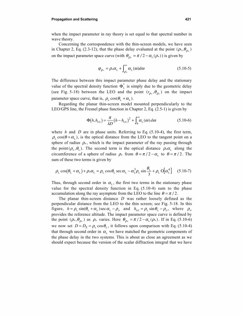
Propagation and Scattering 421
when the impact parameter in ray theory is set equal to that spectral number inwave theory.
Concerning the correspondence with the thin-screen models, we have seenin Chapter 2, Eq. (2.3-12), that the phase delay evaluated at the point ( , )* *
ρ θ ρ
on the impact parameter space curve (with θ π α ρρ* L/ ( )*= −2 ) is given by
ϕ ρ α α ω ωρ ρ* L L*
* ( )= +∞
∫ d (5.10-5)
The difference between this impact parameter phase delay and the stationaryvalue of the spectral density function ΦL
* is simply due to the geometric delay(see Fig. 5-18) between the LEO and the point ( , )
* *rρ ρθ on the impact
parameter space curve, that is, ρ θ αL L Lcos( )+ .Regarding the planar thin-screen model mounted perpendicularly to the
LEO/GPS line, the Fresnel phase function in Chapter 2, Eq. (2.5-1) is given by
Φ h hD
h h dh
, ( )LG LG L( ) = −( ) +∞
∫πλ
α ω ω2 (5.10-6)
where h and D are in phase units. Referring to Eq. (5.10-4), the first term,ρ θ αL Lcos( )+ , is the optical distance from the LEO to the tangent point on asphere of radius ρ* , which is the impact parameter of the ray passing throughthe point ( , )L Lρ θ . The second term is the optical distance ρ α* L along thecircumference of a sphere of radius ρ* from θ π α= −/ L2 to θ π= / 2 . Thesum of these two terms is given by
ρ θ α ρ α ρ θ α α ρ θ ρ αL L L L L L L L LL
L Lcos cos sec sin O*3+( ) + = − + [ ]
34 (5.10-7)
Thus, through second order in α L , the first two terms in the stationary phasevalue for the spectral density function in Eq. (5.10-4) sum to the phaseaccumulation along the ray asymptote from the LEO to the line θ π= / 2 .
The planar thin-screen distance D was rather loosely defined as theperpendicular distance from the LEO to the thin screen; see Fig. 5-18. In thisfigure, h o= + −ρ θ α α ρL L L Lsin( )sec and h oLG L Lsin= −ρ θ ρ , where ρo
provides the reference altitude. The impact parameter space curve is defined bythe point ( , )* *
ρ θ ρ as ρ* varies. Here θ π α ρρ* L/ ( )*= −2 . If in Eq. (5.10-6)
we now set D DS= = ρ θL Lcos , it follows upon comparison with Eq. (5.10-4)that through second order in α L we have matched the geometric components ofthe phase delay in the two systems. This is about as close an agreement as weshould expect because the version of the scalar diffraction integral that we have
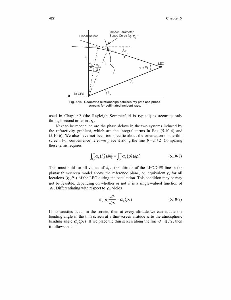
422 Chapter 5
used in Chapter 2 (the Rayleigh–Sommerfeld is typical) is accurate onlythrough second order in α L .
Next to be reconciled are the phase delays in the two systems induced bythe refractivity gradient, which are the integral terms in Eqs. (5.10-4) and(5.10-6). We also have not been too specific about the orientation of the thinscreen. For convenience here, we place it along the line θ π= / 2 . Comparingthese terms requires
α α ρ ρρL L
** *′( ) ′ = ′( ) ′
∞ ∞
∫ ∫h dh dh
S SS*
(5.10-8)
This must hold for all values of hLG , the altitude of the LEO/GPS line in theplanar thin-screen model above the reference plane, or, equivalently, for alllocations ( , )L Lr θ of the LEO during the occultation. This condition may or maynot be feasible, depending on whether or not h is a single-valued function ofρ* . Differentiating with respect to ρ* yields
αρ
α ρL L( ) ( )*
*hdh
d= (5.10-9)
If no caustics occur in the screen, then at every altitude we can equate thebending angle in the thin screen at a thin-screen altitude h to the atmosphericbending angle α ρL ( )* . If we place the thin screen along the line θ π= / 2 , thenit follows that
q L
Fig. 5-18. Geometric relationships between ray path and phase
screens for collimated incident rays.
LEO
q L
aL
aL a
L
rL
aL+
Planar Screen
D
2 2
To GPS
qImpact Parameter
Space Curve ( , )rr* *
r*
r*

Propagation and Scattering 423
h o o= − = −ρ α ρ θ ρ α ρ* *sec sin secL L L (5.10-10)
In a medium with large refractive gradients, thin-screen caustics wheredh d/ *ρ = 0 can arise. The perpendicularly mounted thin screen is not suitablefor these situations.
5.10.2 Duality between Systems
It follows from the previous discussions that when stationary values of thespectral density function exist with respect to spectral number, and when super-refractivity situations are avoided, then we have a kind of duality between thestationary phase processes over spectral number in wave theory and overimpact parameter in geometric optics. For thin-atmosphere conditions awayfrom turning points, rainbow caustics, etc., we may establish a correspondencebetween wave theory and geometric optics when stationary phase values ineach system are assumed. For wave theory applied to a spherical refractingmedium on one hand, and for the scalar diffraction integral applied to a thin-screen proxy for this refracting medium on the other hand, Table 5-1 shows thecorrespondence between these systems when stationary phase values areassigned in each system. Table 5-1 shows this correspondence at a LEOposition. Here G G G† † †( ) [ ( ), ]= ≡ν ρ ν ν , and ρ ν ν ρ
† †( ) ˆ †= − y K .
In summary, a thin phase screen model combined with scalar diffractiontheory gives results that closely match those from wave theory applied to aspherical geometry when (1) caustics do not occur in the thin screen,dh d/ *ρ ≠ 0 , which is related to the thin-atmosphere conditions cited earlier,(2) the observer is relatively far from the refraction zone, and (3) certain LEOrainbow caustic and reflection locations are avoided.
On the other hand, there are situations where wave theory and wave/opticsapproaches give disparate results. One example is when no stationary spectralnumbers occur; this corresponds to super-refractivity in geometric optics or totransition across a shadow boundary. Another example is a caustic contact pointwhere second-order geometric optics predicts infinity for the amplitude of theray and it errs in predicting the exact location of maximum flaring. Wavetheory accurately addresses these cases. Although addressed later, one also canmake a close correspondence between wave theory and geometric optics resultswhen reflections occur.

424 Chapter 5

Propagation and Scattering 425
5.10.3 Amendments to Account for Wave-Front Curvature from theFinite Distance of the Emitting GPS Satellite
Almost all of the discussion in this monograph has assumed an infinitedistance for the emitting GPS satellite. The wave-front curvature effects froman emitting GPS satellite at a finite distance can be accommodated as follows.From geometric optics, see Appendix A, Eq. (A-55), the phase delay along aray, now referenced to the emitting GPS satellite, is given by
ϕ ρ ρ ρ ρ ρ α ρ α ω ωρ
= − + − + +∞
∫L G L L*
* * * *( ) ( )2 2 2 2 d (5.10-11)
Here it is assumed the emitter and the receiver are well out of any refractingmedium. Otherwise, we would have to break the terms involving α L intoseparate parts, one for δ L , the ray path deflection angle at the LEO, and one forδ G , the ray path deflection angle at the GPS, with α δ δL L G= + ; see Fig. A-3.
This form for the phase delay in Eq. (5.10-11) is the eikonal function S ( )rin geometric optics. The eikonal equation is | |∇ =S n, and a constant value forS defines the geometric optics equivalent of a surface of constant phase delayof the electromagnetic wave (essentially a wave-front or cophasal surface).
The main change in wave theory for a finite GPS distance is in theasymptotic form that the incoming spectral coefficients assume for large radialdistances out of the atmosphere. This difference between collimated andspherical incident waves was briefly discussed in Section 5.5, Eqs. (5.5-3a) and(5.5-3b). When one accounts for wave-front curvature, the spectral densityfunction Ψ( , )+ − for an outgoing wave at the LEO [see Eq. (5.9-6)] is amendedto the form (always with θ πG ≡ )
Ψ = − + − + + −( ) − −
=
=
−
−
ρ ν ρ ν ν θ θ θ ν π
θ νρ
θ νρ
ν ν
ν
ν
G LG L
L
G
G
L
L
†( )
sin
sin
2 2 2 2
1
1
24
G
(5.10-12)
Then the stationary value of Ψ( , )+ − , if one exists, is obtained by setting∂ ∂νΨ( , ) /+ − = 0 . This yields
∂∂ν
θ θ θνν ν
Ψ = + −( ) − =G LL
†
2 0dG
d(5.10-13)

426 Chapter 5
Letting Φ ΨL ** ( , ) /= + − +=ν ν π 4 and using Eq. (5.10-3), we obtain
ΦL G L*
G L L L*
* * *†
† *
* * * *
( )
( ) ( )
= − + − +
−
→ − + − + +∞
∫
ρ ν ρ ν νν
ν
ρ ρ ρ ρ ρ α ρ α ω ω
ν
ρ
2 2 2 2
2 2 2 2
2 2dG
dG
d
(5.10-14)
The lower line is obtained by letting ν ρ**→ , and it is in agreement with the
eikonal form in Eq. (5.10-11) given from geometric optics.
5.11 The Electric Field at a Turning Point
At a turning point, r r= * and θ θ= * . We have discussed in Section 5.8 thebreakdown in accuracy of the representation of the field by osculatingparameters when the field is evaluated in the immediate neighborhood of aturning point. When certain scale factors permit, we can accurately approximatethe medium by a spherical Airy layer in the neighborhood of a turning point.We have seen in Sections 4.7 and 4.8 for a Cartesian stratified medium that theosculating parameter approach works well at a turning point when the Airyfunctions are used as basis functions. For the boundary r rA= between the Airylayer below and the medium above, Section 5.8 uses the continuity conditionsfrom electrodynamics to match the osculating parameter solution for r rA≥ tothe Airy solution for r rA≤ .
The Airy layer approximation works well when the effect of curvature inthe refractivity profile is sufficiently small over the width of the layer. Two keyscale factors can permit this approximation. The first is related to ′′ ′n n/ . Foran exponential medium, this factor becomes H −1, where H is the scale height(here in length units). In this case, we want the width of the Airy layer ∆r to besmall enough that, in the power series expansion of the exponentialrepresentation of the medium, the quadratic and higher-order terms in ∆r H/are negligible, i.e., ∆r H/ .<< 1 On the other hand, we don’t want the boundaryr rA= of the Airy layer to be chosen so close to the turning point radius that theaccuracy of the osculating parameter approach has begun to deteriorate, whichoccurs when ˆ ~y > −2 . Using Eq. (5.4-3) to express ∆y in terms of ∆r over thewidth of the Airy layer, we have
∆ ∆y
kH
K
r
HA
= −ρ
(5.11-1)
Thus, the two dimensionless factors permitting an Airy layer approximation arekH and K kn r
A A Aρ = ( )/ /2 1 3; the latter is related to rA / λ . When H

Propagation and Scattering 427
corresponds to the Earth’s dry air conditions ( km)H ≈ 7 and for GPSwavelengths, kH K
A/ ρ ≈ 500 . In this case, we could set ∆r H/ ~ .0 01,
achieving better than 0.01 percent accuracy in the representation of therefractivity by an Airy layer, with a boundary above which the osculatingparameter approach also is sufficiently accurate. We also want to keep ∆ysmall enough that phase runoff in the Airy function approximate solution, givenin Eq. (5.8-6), as compared to the exact solution is negligible. This also isrelated to the size of ′′ ′n n/ .
In matching the solution in the Airy layer involving the Airy function of thefirst kind with the osculating parameters/spherical Hankel functions that holdabove the layer, we apply the continuity conditions from electrodynamics. Thisresults in the matching coefficients cl and dl given in Eq. (5.8-8). We maymultiply these coefficients by any complex factor that we wish [for example,i l l ll ( ) / ( )2 1 1+ + ], provided that we apply that factor to both coefficients or,equivalently, to both the incoming and outgoing components of the field. Also,
at the boundary the outgoing phase term 2G G Aρ ν ρ ν†, ,[ ] − [ ], which is givenin Eq. (5.8-24), must equal the exact value of the round-trip phase delaythrough the Airy layer. This fixes ρ† at the Airy layer boundary perEq. (5.8-15). For a given value for l , the asymptotically exact value for theround-trip phase delay through an Airy layer is given by Eqs. (5.8-12) and(5.8-13). Fortunately, we need not explicitly apply this condition; we need onlythe representation by the Airy function of the first kind at the turning point. Butin practice the numerical integration of these wave equations has a stabilityproblem below the turning point. The slightest phase error in the initialconditions at the boundary r rA= results in a blowup below the turning pointor, equivalently, to a leakage of the Airy function of the second kind into thenumerical solution. See the discussion of the WKB solutions and Eq. (5.7-26).
Near a turning point, we start with the integral version of the spectralrepresentation for the field given in Eq. (5.8-1b). Because we are evaluating thefield near a turning point, we do not have unrestricted use of the negativeargument asymptotic form for the Airy function. But we still can use thenegative exponential form for the Legendre function, which generally isapplicable for large spectral numbers and for 0 < <θ π .
We replace the form a al l l l− − + +ξ ξ+ in Eq. (5.8-1) with Ai[ ˜]y times a
spectral number-dependent coefficient. When the negative argument asymptoticforms hold at the boundary of the Airy layer, we have from Eq. (5.8-8) theconnecting relationship between the solution below the boundary and thesolutions above the boundary. This is given by
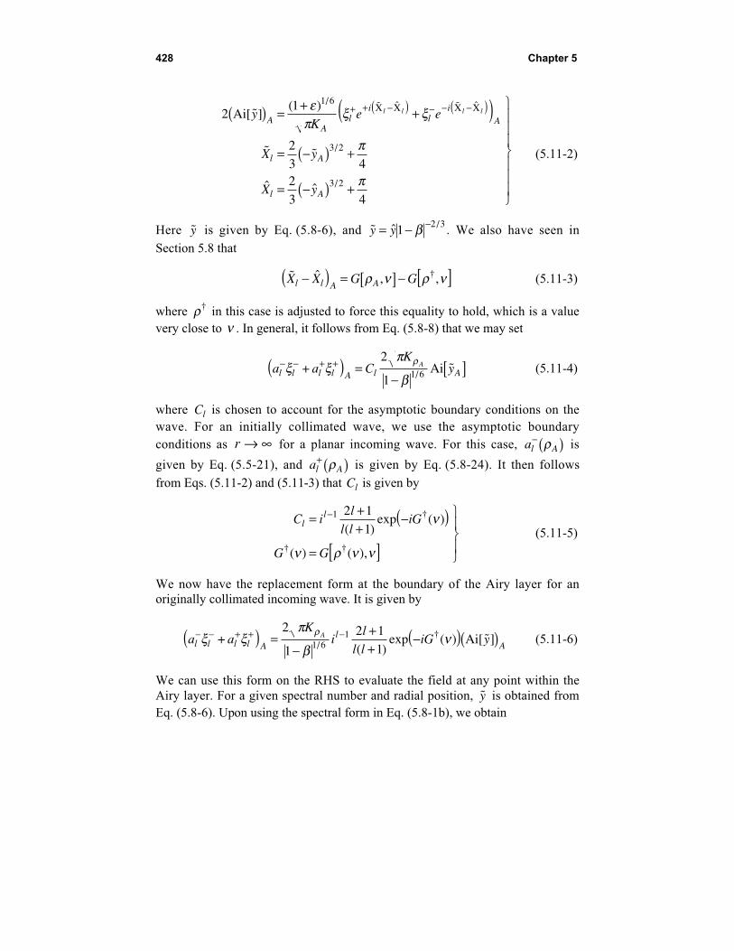
428 Chapter 5
21
23 423 4
1 6
3 2
3 2
Ai[ ˜]( )
˜ ˜
ˆ ˆ
/ ˜ ˆ ˜ ˆ
/
/
yK
e e
X y
X y
AA
li
li
A
l A
l A
l l l l( ) = + +( )= −( ) +
= −( ) +
+ + −( ) − − −( )επ
ξ ξ
π
π
Χ Χ Χ Χ
(5.11-2)
Here y is given by Eq. (5.8-6), and ˜ ˆ /y y= − −1 2 3β . We also have seen inSection 5.8 that
˜ ˆ , ,†X X G Gl l A A−( ) = [ ] − [ ]ρ ν ρ ν (5.11-3)
where ρ† in this case is adjusted to force this equality to hold, which is a valuevery close to ν . In general, it follows from Eq. (5.8-8) that we may set
a a CK
yl l l l A l AA− − + +( ) =
−[ ]ξ ξ
π
βρ
+2
1 1 6/ Ai ˜ (5.11-4)
where Cl is chosen to account for the asymptotic boundary conditions on thewave. For an initially collimated wave, we use the asymptotic boundaryconditions as r → ∞ for a planar incoming wave. For this case, al A
− ( )ρ is
given by Eq. (5.5-21), and al A+ ( )ρ is given by Eq. (5.8-24). It then follows
from Eqs. (5.11-2) and (5.11-3) that Cl is given by
C il
l liG
G G
ll= +
+−( )
= [ ]
−1 2 11( )
exp ( )
( ) ( ),
†
† †
ν
ν ρ ν ν(5.11-5)
We now have the replacement form at the boundary of the Airy layer for anoriginally collimated incoming wave. It is given by
a aK
il
l liG yl l l l A
lA
A− − + + −( ) =−
++
−( )( )ξ ξπ
βνρ
+2
1
2 111 6
1/
†
( )exp ( ) Ai[ ˜] (5.11-6)
We can use this form on the RHS to evaluate the field at any point within theAiry layer. For a given spectral number and radial position, y is obtained fromEq. (5.8-6). Upon using the spectral form in Eq. (5.8-1b), we obtain

Propagation and Scattering 429
EK
Ey e d
EK
iEy e
ro
i G
oi
( ˜ , )sin
Ai[ ˜] ,
( ˜ , )sin
Ai [ ˜]
/ / ( )
/ /
*
†
*
ρ θβ
θνρ
ν
ρ θβ
θνρ
ρ
ν π θ ν
θρ
ν π θ
=−
=−
′
− − −
∞
− − −
∫1
1
1 6 3 22
0
1 6
2
1 22
GG
A
d
yK
l
kn rn
dn
dK
†
*
*
*
( )
/ * *
**
/
,
˜ ( )( ˜ ) ( ) ,
˜ , ˜
˜ , , ˜ ˜
ν
ρ
ρρ
ν
ββ ρ ρ ρ
ρ βρ
ρ ρ ρ ρ
∞
∫
= −−
− − − −( )
= = −
=
≤
0
2 3
1 3
1
11
12
(5.11-7)
The constant gradient of the refractivity in the Airy layer, ′ =n dn d/ ρ , is set bythe actual values of n( )ρ at the turning point r* and at the boundary at r rA= .Thus, the gradient of the refractivity will be discontinuous at the boundary, butrefractivity itself will be continuous.
5.11.1 Fourier Transform of the Airy Function
We have seen in previous sections on stationary phase processes that, neara turning point and at the stationary phase value in spectral number,dG dρ ρ ρ ρ α ρ ρ†( ), / ˙ ˜ ( , )* * * * *[ ] = with very high accuracy for thin-atmosphereconditions. But for now let us consider the integrals in Eq. (5.11-7) as Fouriertransforms. When throughout the medium n( ) constantρ = , then G[ , ]ρ ν ≡ 0 orat most a constant; it can be removed from the integrands in Eq. (5.11-7). From[8], we have the integral representation for the Airy function:
Ai[ ˆ]( )
exp ( ) ˆ/
/ya
i at a yt dt= +( )( )−∞
∞
∫32
31 3
3 1 3
π(5.11-8)
where a is any positive constant. It is easy to show that this integral formsatisfies the differential equation for the Airy function Ai ˆ Ai′′ = y . Using theDirac delta function,
δ ωπ
ω( ) exp= ( )−∞
∞
∫12
i t dt (5.11-9)
it follows from Eqs. (5.11-8) and (5.11-9) that the Fourier transform of Ai[ ˆ]y isgiven by
Ai[ ˆ]exp ˆ ˆ expy i y dyiω ω( ) = −
−∞
∞
∫3
3(5.11-10)

430 Chapter 5
If we set ω π θρ= −K ( / )2 and we use the approximation ν =
ρ ρ ρ+ +K y y Kˆ ˆ /2 60 [see Eq. (5.4-3)], then we obtain
Ai[ ˆ] ˆ ˙( / ) / ( / ) / ! ( / ) / ! cosy dy e ei i ie ν π θ ρ π θ π θ π θ ρ θ2 2 2 3 2 53 5−−∞
∞ − − − + −( )∫ = = (5.11-11)
Thus, the Fourier transform of the Airy function of the first kind, at least near aturning point, is the phasor associated with the optical path length along the raymeasured from the turning point, hardly a surprising result.
We can carry the Fourier transform approach a bit further and apply it tothe radial component of the electric field in Eq. (5.11-1) for the case of thehomogeneous medium where G[ , ]ρ ν ≡ 0 . Again using the Dirac delta function
and its derivatives, it can be shown upon expanding the term ( / ) /l ρ 3 2 inpowers of y that
1 3 22
sinAi( ˆ) ˆ ˙ sin
// cos
θ ρθν π θ ρ θl
y e dy ei i
=−( )−∞
∞
∫ (5.11-12)
which we already know from physical considerations to be true.Returning to the stratified case in Eq. (5.11-7), we now evaluate the radial
component of the field at the turning point Er ( , )* *ρ θ , where
θ π α ρ ρ* * */ ˜ ( , )= −2 . We expand G[ , ]†ρ ν in powers of spectral number aboutthe given value ρ* where ( [ ( ), ] / ) ˙ ˜ ( , )†
* * *dG dρ ν ν ν α ρ ρρ = . We also make a
change of variable in the integration from ν to y using Eq. (5.11-7). We obtain
E E e yi d
ddy
G kr n
d
d
d
r oi
( , ) ˙cos ˜
Ai[ ˜]exp˜
( ) ˜,
˜ ( ), , ( ),
˜ , ˜ ˜ ( ,
* **
*
**
* *†
* * * * *
* *
*
*
ρ θ βα
αρ
ν ρ
ρ α ρ ρ ρ ρ ρ
θ π α αρ
α ρ
ρ
ρ
= − − −
= − [ ] =
= − =
−∞
∞
∫12
2
2Φ
Φ
ρρρ
α α ρ ρ
ν ρ β βρ
ρ ρρρ
), ˜ ˜ ( , ),
˙ ˜( ) , ˜
˜ , ˜
* * *
*/
**
*
d
y Kn
dn
dkn r
=
= + − = −
=
112 3
(5.11-13)
We note the phase term Φ ρ*. It may be written as
Φ ρ ρρ α ρ ρ ρ ρ ρ ρ α ρ ρ α ω ω ω
**
* * *†
* * * * *˜ ( , ) ( ), ˜ ( , ) ˜ ( , )= − [ ] = +∞
∫G d (5.11-14)

Propagation and Scattering 431
The first term is simply an optical path length along the circular arc of radiusρ* measured from the reference point (θ π= / 2 ) to the angular positionθ π α= −/ ˜*2 . The second term, from Eq. (5.7-6), is the phase retardationinduced by the gradient in the refractivity that the ray incurs in travelingthrough the atmosphere to the tangency point at r*.
The quadratic term in the integral in Eq. (5.11-13) involvingd G d d d2 2/ ˜ /ν α ν= is related to the defocusing of the incident collimatedwave resulting from the gradient of the refractivity.
5.11.2 Fresnel Transform of the Airy Function
To obtain the Fresnel transform of the Airy function, we again use theintegral form for the Airy function given by Eq. (5.11-8). We obtain
Ai[ ˜]exp ˜ ˜ ˜ ˜/ ( ) ˜ ˜y i y y d y e e dy dziz i z y yσ τπ
σ τ+( )( ) =
−∞
∞
−∞
∞ + +( )−∞
∞
∫ ∫ ∫2 312
3 2
(5.11-15)
Here σ and τ are constants. From Eq. (5.11-13), it follows for our case that
τ β αρρ= − −( )1
212 4 3K
d
d*
/
*
˜(5.11-16)
Equation (5.11-15) is a more general version of the Fresnel transform; the latteris obtained by setting σ = 0 . Upon completing the square in the inner integralof Eq. (5.11-15), one can write it in terms of the complete Fresnel integral.Then with a change of variable and the use again of the integral form for theAiry function given in Eq. (5.11-8), one finally obtains
Ai[ ˜]exp ˜ ˜ ˜| |
Ai[ ]expy i y y dy b icσ τ πτ
+( )( ) = ( )−∞
∞
∫ 2 (5.11-17)
where
b
c
= − +
= ± + − +
1 8
16
41
192
1 4
64
2
3
2
3
σττ
πτ
σττ
( )(5.11-18)
Here +π / 4 is used in the expression for c when τ > 0 , and −π / 4 is usedwhen τ < 0 . Thus, the Fresnel transform of the Airy function yields an Airyfunction again but with offsets in phase and argument and with a modifiedamplitude. We note the defocusing term | |τ appearing in the denominator ofEq. (5.11-17).

432 Chapter 5
Using the Fresnel transform of the Airy function, the value of the integralin Eq. (5.11-13) becomes
EE
b i cro( , )
cos ˜ | |Ai[ ]exp* *
/
**
ρ θβα
πτ ρ=
−+( )( )1 1 2
Φ (5.11-19)
We note that, for thin-atmosphere conditions, τ << 1. For an exponentialatmosphere,
τπ
β βρ= −
−1
41
1 24 3K
kH*
//( ) (5.11-20)
For GPS signals with dry air at sea level, τ ~ 10 3− . In this case, Eq. (5.11-17)essentially collapses to unity as τ → 0 and for σ = 0 . In this case,Eq. (5.11-19) reduces to the form
EE
iro( , )
cos ˜exp* *
/
**
ρ θβα ρ=
− ( )1 1 2
Φ (5.11-21)
We see the defocusing factor 1 1 2− β / appearing here. Squaring this factoryields the defocusing in signal power, which essentially agrees withEq. (5.6-16), the prediction from geometric optics for the defocusing at aturning point.
For Eθ , one can use the Fresnel transform of Ai [ ˆ]′ y to derive similarresults. Eθ should be essentially zero at a turning point. Also, the integral ofAi [ ˆ]′ y over the real axis is zero.
5.12 Caustics and Multipath
Whether or not there is a unique ray, or possibly no ray, arriving at thepoint ( , )r θ depends on the nature of the profile of n( )ρ , which may or may notresult in caustics for the ray system and consequent multiple ray paths withinthe multipath zone. We have discussed caustics and their effects in Chapters 2and 3, and they arise again here. These chapters also show examples of theconverse of a multipath zone: the shadow zone, which in second-ordergeometric optics is a zone devoid of rays in the limit and extreme defocusing inactuality. A shadow zone based on geometric optics has an analog in wavetheory. In shadow zones, wave theory using the spectral integrals inEqs. (5.8-1) or (5.9-24) predicts much-diminished amplitudes for the field, butnot zero. Also, wave theory accounts for diffraction. Using the stationary phasetechnique, it is readily shown that, in a strict shadow zone in geometric optics,the wave theory spectral integrals have no stationary phase points in spectral

Propagation and Scattering 433
number; thus, a small but non-zero fluctuating amplitude results. In the thin-screen model, geometric optics predicts no rays within a shadow zone, but thescalar diffraction integral from a thin screen yields a small but non-zeroamplitude in this zone. The scalar diffraction integral applied to a thin screenintegrates the path delay phasor over impact parameter space in the thin screen.Section 5.10 discussed the close correspondence between stationary phasevalues of spectral number in wave theory and stationary phase values of impactparameter in the scalar diffraction/thin screen. Under most conditions, thescalar diffraction/thin-screen model generates essentially the same values forthe electromagnetic field at a point well away from the screen, includingdiffraction effects, that are obtained from wave theory using the spectraltechnique described here.
We have already shown a specific example without caustics in Fig. 5-10 fora monotonic profile for the refractivity, the exponential profile given inEq. (5.8-2a). In that example, for a given position ro ,θ( ) , the stationary phasecondition on wavenumber in Eq. (5.9-11) is satisfied uniquely at theintersection of the δ and ∂ ∂νG / curves versus ν . These curves are generatedfrom Eqs. (5.9-14) and (5.7-7), respectively, for several values of θ , and theyapply to an incoming region. The curve for ∂ ∂νG / (and implicitly the δcurve) in Fig. 5-10 uses a refraction profile that corresponds closely to thephysical conditions for the dry air component of the Earth’s atmosphere with rocorresponding to sea level. The value of ν at the intersection point of the∂ ∂νG / and δ curves is essentially the impact parameter at the Earth’s surface.Fixing ro ,θ( ) to a different pair of values would cause displacements of the δcurve (see Eq. (5.9-14)) and the ∂ ∂νG / curve (see Eq. (5.7-7)) and, therefore,to an intersection at a different bending angle ˜ ,α ρ νo( ) , which yields a differentν value.
5.12.1 A Numerical Example of Multipath and Caustics
As a simple first example, we consider the refractivity profile fromEq. (5.8-2b), where n( )ρ has a non-super-refracting Gaussian distribution. Amore realistic case, to be considered later, embeds this distribution in abackground distribution corresponding to the near-exponential form for dry air.This dry air distribution causes significant defocusing, which has the effect ofgreatly compressing the bending angle spread from the multiple rays.
In the case of a Gaussian refractivity profile, d d˜ /α ρ is not monotonic,and, therefore, caustics and multipath arise for certain positions ( , )r θ . We usethe refractivity profile given by Eq. (5.8-2b) to obtain the electric field at theLEO. When this Gaussian profile is used in Eq. (5.6-5), a bipolar bending-angleprofile results, ˜ ( , )* *α ρ ρ (see Appendix E). The total refractive bending angleat the LEO is α ρ α ρ ρL ( ) ˜ ( , )* * *= 2 .
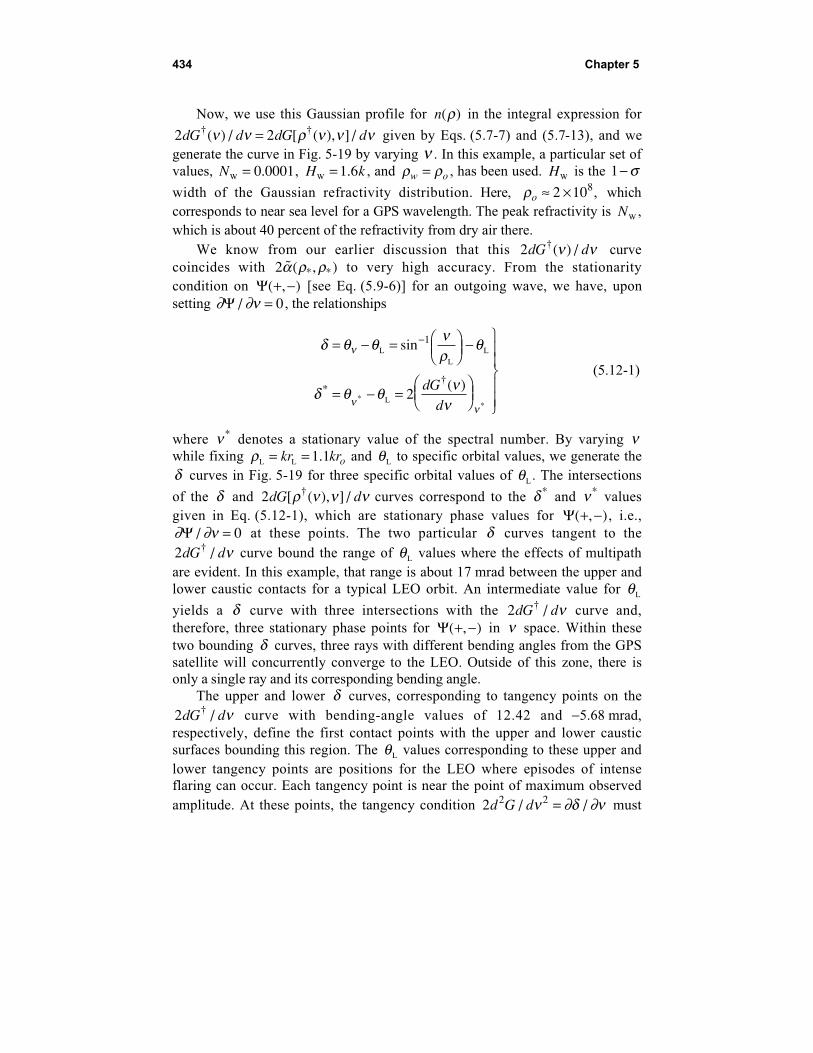
434 Chapter 5
Now, we use this Gaussian profile for n( )ρ in the integral expression for
2 2dG d dG d† †( ) / [ ( ), ] /ν ν ρ ν ν ν= given by Eqs. (5.7-7) and (5.7-13), and wegenerate the curve in Fig. 5-19 by varying ν . In this example, a particular set ofvalues, NW .= 0 0001, H kW .= 1 6 , and ρ ρw o= , has been used. HW is the 1 − σwidth of the Gaussian refractivity distribution. Here, ρo ≈ ×2 108, whichcorresponds to near sea level for a GPS wavelength. The peak refractivity is NW ,which is about 40 percent of the refractivity from dry air there.
We know from our earlier discussion that this 2dG d†( ) /ν ν curvecoincides with 2 ˜ ( , )* *α ρ ρ to very high accuracy. From the stationaritycondition on Ψ( , )+ − [see Eq. (5.9-6)] for an outgoing wave, we have, uponsetting ∂ ∂νΨ / = 0 , the relationships
δ θ θ νρ
θ
δ θ θ νν
ν
νν
= − =
−
= − =
−L
L
L
* L*
sin
( )*†
1
2dG
d
(5.12-1)
where ν * denotes a stationary value of the spectral number. By varying νwhile fixing ρL L .= =kr kro1 1 and θL to specific orbital values, we generate theδ curves in Fig. 5-19 for three specific orbital values of θL . The intersections
of the δ and 2dG d[ ( ), ] /†ρ ν ν ν curves correspond to the δ * and ν * valuesgiven in Eq. (5.12-1), which are stationary phase values for Ψ( , )+ − , i.e.,∂ ∂νΨ / = 0 at these points. The two particular δ curves tangent to the2dG d† / ν curve bound the range of θL values where the effects of multipathare evident. In this example, that range is about 17 mrad between the upper andlower caustic contacts for a typical LEO orbit. An intermediate value for θL
yields a δ curve with three intersections with the 2dG d† / ν curve and,therefore, three stationary phase points for Ψ( , )+ − in ν space. Within thesetwo bounding δ curves, three rays with different bending angles from the GPSsatellite will concurrently converge to the LEO. Outside of this zone, there isonly a single ray and its corresponding bending angle.
The upper and lower δ curves, corresponding to tangency points on the2dG d† / ν curve with bending-angle values of 12.42 and −5.68 mrad,respectively, define the first contact points with the upper and lower causticsurfaces bounding this region. The θL values corresponding to these upper andlower tangency points are positions for the LEO where episodes of intenseflaring can occur. Each tangency point is near the point of maximum observedamplitude. At these points, the tangency condition 2 2 2d G d/ /ν ∂δ ∂ν= must

Propagation and Scattering 435
hold. From Eq. (5.12-1), we have ∂δ ∂ν ν/ /= 1 D , where Dν ρ ν= −L2 2 . The
defocusing factor at the LEO for a tangency point is given byζ νν
− = − =1 2 21 2 0D d G d/ (see Eq. (5.9-29)), which defines a caustic contact
point. Setting ν ν ρ= =** , we conclude that a condition for no caustics is given
by 2 2 12 2d G d d d D†*/ ˙ ˜ / /
*ν α ρ ρ= < for all ρ* values. Therefore, the gradient
of the bending angle can be positive, but not too positive, less than about0 3. mrad km/ for a GPS wavelength and with r roL .≈ 1 1 . We also note that, incases where the refractivity gradient is continuous, the number of multipathrays is odd, except at a caustic contact point.
If these stationary phase points are adequately separated in wavenumber(see Appendix D for an “adequacy” index), then geometric optics as anapproximate technique should suffice, which treats them as corresponding toseparate rays. Geometric optics can be used with Eq. (5.6-5) to generate the ray
for the impact parameter value ρ ρ ν* *†= ( ) corresponding to each of these
intersection points. The phasors for three rays can be combined as vectors, i.e.,taking into account their relative phases and amplitudes to obtain the aggregateelectric field at the point rL L,θ( ) . However, near the caustic limits, two of these
points will merge, and geometric optics will become inadequate for stationaryphase points in spectral number that are in the neighborhood of the causticcontact point. In wave theory, the second-order stationary phase technique for
5
Fig. 5-19. Wave theory multipath zone in spectral number for a Gaussian
refractivity profile. The phasor exp(iY(+,-)) in the spectral integral is
stationary at an intersection of the and 2dG†/d curves, which gives the
bending angle of the corresponding ray. Tangent points are caustic
contacts where ∂Y/∂ = ∂2Y/∂ 2 = 0.
d d qn L or + D= ( , ,
)
d d qn L or - D= ( , ,
)
d d qn L or= ( , , )
D = ~ 8 mrad
La = -5.68, 0
La = 0, 12.42
mra
d
n r- )/(o
Hw
-4 42
10
-2
-5
-6-8
2dG ,[ ]/d† nr n
2 ~a d n
n n
La = -0.55, 3.33, 4.56

436 Chapter 5
evaluating the integrals in Eq. (5.8-1b) over spectral number also becomesinadequate for the same reason. These spectral integrals should be directlyevaluated, or a third-order stationary phase technique can be used, such as thatdescribed in Appendix D and discussed later in this chapter.
A caustic contact historically is associated with laser-like rays, for example,a rainbow spectral component from a water drop. Whether or not that kind offlaring in signal amplitude actually occurs at a caustic depends on the curvatureof the 2dG d† / ν curve; that is, it depends on the magnitude of ∂ ∂ν3 3Ψ( , ) /+ −at the caustic contact point ν ν= * , where ∂ ∂ν ∂ ∂νΨ Ψ( , ) / ( , ) /+ − = + − =2 2 0 .If the magnitude of ∂ ∂ν3 3Ψ( , ) /+ − is relatively small at the caustic point, thena broader neighborhood of spectral numbers about the stationary phase pointcontributes constructively to the spectral integral evaluation. This results in alarger amplitude. In other words, the spectral width about a stationary phasepoint across which phase coherence in the integrand is preserved dependsinversely on ∂ ∂ν3 3Ψ( , ) /+ − when both ∂ ∂νΨ( , ) /+ − and ∂ ∂ν2 2Ψ( , ) /+ − areat or near zero. We will show later that the amplitude of the flaring at a causticcontact point is proportional to ( ( , ) / ) /∂ ∂ν3 3 1 3Ψ + − − . If the amplitudes of thenew rays created at a caustic contact point are relatively strong, then signalflaring is to be expected even if interference is present from a pre-existing ray.If the amplitudes of the new rays are relatively weak, then the pre-existing raywill be dominant and the signal flaring, such as it is, will show up on theenvelope of the resulting interference fringes. The Gaussian refractivity profileused in this section yields the latter scenario. Section 5.13 and Chapter 6provide examples of the former scenario with very strong nascent rays.
Figure 5-20 shows the relationship between LEO orbital angle θL andimpact parameter ρ* from geometric optics for the same Gaussian refractivityprofile and orbit model used in Fig. 5-19. This impact parameter diagram isobtained directly from Bouguer’s law, θ ρ ρ α ρ ρL Lsin / ˜ ( , )* * *= ( ) −−1 2 . Oncethe refractivity profile is specified, ˜ ( , )* *α ρ ρ is obtained from Eq. (5.6-5). For− ≤ − ≤12 2 4 8. .Lθ θo , a triplet of impact parameter values and bending anglessimultaneously satisfies the boundary conditions provided by the positionrL L,θ( ) of the LEO. Significant multipath occurs within this zone. Caustic
contacts lie at the points where d dθ ρL
/ * = 0 . These points correspond toepisodes of signal flaring, and they mark the boundaries of the multipath zone,in this example at θ θL .− =o 4 8 and at θ θL .− = −o 12 2 . Above θ θL .− =o 4 8 ,the rays labeled (a) and (b) are non-existent in a second-order geometric opticscontext. Only the ray labeled (m) exists. Similarly, rays (m) and (a) do not existbelow θ θL .− = −o 12 2 ; only (b) rays exist.
Propagation and Scattering 437
For the occulted GPS satellite lying in the orbit plane of the LEO andsetting , θL decreases with time at a rate of roughly 1 mrad/s. Therefore, eventsunfold in Fig. 5-20 from right to left for a setting occultation. Aboveθ θL .− =o 4 8 , only one stationary phase value in spectral number is realized.There is a unique value for any given orbit angle above this limit. This uniquesequence of stationary phase values in spectral number versus θL above thislimit corresponds in geometric optics to the impact parameter branch (m) in thefigure, which defines the tangency points or impact parameter values generatedby the (m) family of stationary phase paths, the (m) rays. When θ θL − o dropsbelow 4.8 mrad, the first contact with a caustic is made. This results in flaringof the signal and the onset of interference from the triplet of competingstationary phase points in spectral number. In geometric optics, thiscorresponds to the existence of three competing ray systems, (m), (a), and (b); amember from each family passes through the position of the LEO. See Fig. 2-3for a ray diagram. Ray (a) is the anomalous ray, and although it is a path ofstationary phase, it can be shown that this path provides a local maximum inphase delay. Paths (m) and (b) provide local minima. This multipath episodecontinues until the lower caustic contact point is reached at θ θL .− = −o 12 2 .Below this point, a single stationary phase value in spectral number resumes,corresponding to the lower main ray (b) and the resumption of a smooth signal.
Figure 5-21(a) shows the signal amplitude E rL L,θ( ) at the LEO versus
orbit angle θ θL − o for the same models used in Figs. 5-19 and 5-20. This figure
Fig. 5-20. Impact parameter diagram from geometric optics. This figure
shows versus LEO orbit angle in the neighborhood of the same
refracting layer described in Fig. 5-19. Labels (m), (a), and (b) identify the
corresponding rays: main, anomalous, and branching.
r Lo roo
r Lrq
=
= ¥
1.6k, r =
==
rLk
k 3.32
LHw
410 -1km
(m)
(a)
(b)
,sin 1.1
Lq
Lq
oq- (mrad)
rr
-)/
(o
Hw
*
r*
-7.5-10.0 5.02.5
-7.5
-10.0
-2.5
7.5
5.0
-5.0
-5.0 -2.5
2.5

438 Chapter 5
Fig
. 5
-21
. A
mp
litu
de
of
the
fie
ld a
t th
e L
EO
ve
rsu
s o
rbit
an
gle
fo
r th
e s
am
e o
rbit
mo
de
l a
nd
Ga
us
sia
n
refr
ac
tiv
ity
p
rofi
le
us
ed
in
F
igs
. 5
-19
a
nd
5
-20
: (a
) a
mp
litu
de
o
ve
r th
e
en
tire
m
ult
ipa
th
zo
ne
a
nd
(b)
am
pli
tud
e i
n t
he
vic
init
y o
f th
e u
pp
er
an
d l
ow
er
ca
us
tic
co
nta
ct
po
ints
.
−11
−11
.5−1
2
0.5
1.0
1.5
2.0
(b)
rθ LL , E()
θ Lθ o
–
#
5.0
2.5
0.0
(a)
−2.5
−5.0
−7.5
−10
.0−1
2.5
rθ LL , E()
θ Lθ o
–(m
rad
)
1.5
2.0
1.0
0.5
5.2
4.8
4.6
4.4
4.2
4.0
0.0
0.5
1.5
2.0
r θ L L,E ( )
θ Lθ o
–
1.0

Propagation and Scattering 439
was obtained from a numerical integration of the spectral integral for Er givenin Eq. (5.8-1b) or, equivalently, Eq. (5.9-10). The numerical integration wasaided by the stationary phase technique to isolate stationary phaseneighborhoods, thereby reducing the computational burden11 (see Section 2.6).The spectral coefficient al
+ ( )ρ used in the integration is given in Eq. (5.8-25),
and G G† †( ) ( ),ν ρ ν ν= [ ] is given from Eq. (5.7-2), using the refractivity profilegiven in Eq. (5.8-2b) and the parameter values used for Figs. 5-19 and 5-20.Figure 5-21(a) shows the smooth and nearly constant signal amplitude outsideof the multipath zone, and it clearly shows the abrupt onset of a multipathepisode at the upper caustic contact point at about θ θL .− ≈o 4 8 , continuinguntil the lower contact point at θ θL .− ≈ −o 12 0 . This figure demonstrates theviolent interference from a triplet set of stationary phase points that can resultfrom a non-monotonic refractivity profile if the refractive gradient is evenmoderate in magnitude. Caustic flaring at the contact points is almostimmediately overwhelmed by phase interference among the three full-fledgedstationary phase paths. In this example, inspection of the gradients in bendingangle in the middle of the multipath zone in Fig. 5-20 shows that none of thepaths is overly defocused relative to its competitors. Defocusing is evident in theneighborhood of θ θL − =o 0 because of the steep gradients in bending angle on allthree rays there. Above θ θL − =o 5, the principal contribution to E rL L,θ( ) comesfrom the main ray (m) without interference from the (a) and (b) rays (seeFig. 5-20). Below this point, three mutually interfering ray paths contribute to thespectral integrals. Contact with the lower caustic occurs at θ θL .− ≈ −o 12 2 .Abrupt termination of the scintillation episode follows. Below this only the (b) rayremains to contribute to E rL L,θ( ).
Figure 5-21(b) is a blowup of the neighborhoods around the upper andlower caustic contact points to show the fast and slow fringes in amplitude ofthe field at the LEO. The high-frequency fringes from interference betweenrays are resolved at the upper contact point; at the lower point, their spacing isless than the resolution of the figure. The lower contact point shows somewhatless flaring than the upper point. Figure 5-20 shows that d d2 2θ ρL / * issomewhat larger at the lower point than at the upper point. It will be shown thatd d2 2 3 3θ ρ ∂ ∂νL / ( , ) /* = + −Ψ when ν ρ= * . It follows that when d d2 2θ ρL / * is
larger, the near-tangency condition between the 2dG d†( ) /ν ν curve and the δ
11 Here one uses the stationary phase technique to find all spectral numbers that yield astationary value in Ψ( , )+ − , in this example a maximum of three. Then in Eq. (5.9-24)it is necessary only to carry out a numerical integration over a suitable neighborhoodaround each of these spectral numbers, taking care to properly phase-connect theseseparate converged integration intervals.

440 Chapter 5
curve near a caustic contact point runs over a shorter interval in spectralnumber. Therefore, a smaller contribution to the spectral integral for E rL L,θ( )comes from the spectral neighborhood around the lower caustic point inFig. 5-21(b) than from the neighborhood around the upper caustic point. Thepeak amplitudes near caustic contacts are slightly offset, 0.1 to 0.2 mrad, from thegeometric optics predictions for caustic contact (i.e., where ζ → ∞ ).
Figure 5-22 shows the difference in phase near the upper caustic pointbetween the complete field at the LEO and the field from only the (m) ray. Thespikes of large phase acceleration in this figure correspond to orbit angles inFig. 5-21(b) where the complete field is almost totally annihilated throughmutual interference between the three rays. The frequency of the phase fringesin Fig. 22 scales with impact parameter separation of the rays, which in turnscales roughly linearly with the 1 − σ width of the Gaussian refractivity profile. Fastfringes are from interference between the main ray (m) and the nascent rays (a) and(b). Slow modulation or banding results from interference between the (a) and (b)rays as their impact parameters begin to separate near the caustic point.
5.12.2 A Geometric Optics Interpretation of Multipath
Geometric optics can accurately predict many of the fringe features formultipath situations, such as those shown in Figs. 5-21 and 5-23. One must takeinto account the amplitudes of the competing rays and their phase interferenceas the orbit angle or, equivalently, time evolves. A notable exception is thefailure of geometric optics to accurately predict the field in the immediate
-0.4
-0.2
0.0
5.04.84.64.44.24.0
0.2
0.4
Fig. 5-22. Phase difference near the upper caustic, expressed in cycles of
the complete field at the LEO minus the field of the (m) ray.
qL
qo
–
Ym
ab -
Ym
(cycle
s)

Propagation and Scattering 441
vicinity of a caustic contact. Second-order geometric optics predicts an infiniteamplitude at such places, whereas wave theory gives the correct values.
We now apply geometric optics to see how well it does at predicting thefringe amplitudes and frequencies shown in Fig. 5-21. Starting with Bouguer’slaw, and given our specific refractivity and orbit models, the impact parametercurve for each competing ray system can be calculated. From the impactparameter diagram in Fig. 5-20, one can determine the defocusing of any rayversus orbit angle and also the interference frequencies between any two rays.To interpret the fringes, we need the relative phase changes and amplitudes ofthese competing rays evaluated at the LEO.
For the phase change or excess Doppler, we start with the stationary valueof the spectral density of the phase at the LEO. From Eqs. (5.9-6) and (5.12-1),it is given by
Ψ* * *
* *
( , ) ,
, sin
* * L†
* L L *
+ − = + −( ) − ( ) −
= − =
D G
D
ν ν
ν ν
ν θ θ ν π
ρ ν ν ρ θ
24
2 2(5.12-2)
where G G† †( ) [ ( ), ]ν ρ ν ν= is given in Eq. (5.7-2) with ρ ν ρ† †ˆ †= − y K . Here
we evaluate Ψ( , )+ − at a stationary value Ψ*( , )+ − with respect to spectralnumber. That spectral number ν * is allowed to assume the value of the impactparameter ρ* at a given epoch for a specific ray, either (m), (a), or (b) as shown
in Fig. 5-20. We know from spectral theory that ν * will be very close to ρ* for
that ray, away from super-refracting conditions. Now we differentiate Ψ*( , )+ −with respect to time. Both the orbital position of the LEO and the impactparameter change as time evolves.12 Since we are interested only in thedifference in phase between rays, we can neglect the Doppler term from theobserved GPS satellite. Thus, we have
12 We also should include the obliquity effect resulting from the GPS satellitesgenerally not lying in the LEO orbit plane. This correction factor is discussed inChapter 6. It can reduce Doppler values by up to about 35 percent for inclination anglesup to 30 deg. Here we assume that the occulted GPS satellite lies in the orbit plane ofthe LEO. This assumption essentially impacts only the scale factor between LEO orbitangle change and elapsed time.
442 Chapter 5
d
dt
D dG
d
Ψ Ψ Ψ Ψ* * * *
*
* *
†
L
L
L
L
*
L
L L L*
*
˙ ˙ ˙
˙ ˙ ˙
= + +
= − + − −
=
∂∂ρ
ρ ∂∂θ
θ ∂∂ν
ρ
ρρ ρ θ ρ θ θ
νρ
νν ρ
2
(5.12-3)
But, at a stationary phase point in spectral number, θ θ νν − − =L† /2 0dG d ,
and for a circular orbit ρL ≡ 0 . It follows in this case that
d
dt
d
d
Ψ Ψ*
*
*
*˙ orL
L
= − = −ρ θθ
ρ (5.12-4)
Thus, d d( ) /* *∆Ψ ∆θ ρL = − , where ∆ρ* is the difference in impact parametervalues between any two of the three rays, (m), (a), or (b), at a given epoch ororbit angle, and ∆Ψ* is the difference in phase at the LEO between these tworays. These impact parameter differences can be read directly from Fig. 5-20.The high-frequency fringes in Fig. 5-21(b) near θ θL − =o 5 result frominterference between the combined but relatively weak13 (a) and (b) rays withthe strong (m) ray. At θ θL .− =o 4 8 , the difference in altitudes of the impactparameters between the (m) ray and the nascent (a) and (b) rays is 16.3 km.Thus, the frequency of the fringes resulting from phase interference betweenthese two ray systems is given by ( ) / . /m ab L2 16 31π θ λ− −( ) =d dΨ Ψ* * , orabout 82 cycles/mrad. Although difficult to measure precisely in Fig. 5-21(b),the high-frequency fringe rate is indeed about 80 cycles/mrad. At the lowercaustic contact point near θ θL − = −o 12 , the high-frequency fringes are causedby interference between the (b) ray and the dying (m) and (a) rays (or nascentrays for a rising occultation). Figure 5-20 shows a much wider separation inimpact parameter values there between the (b) ray and the (m) or (a) ray. Thehigh-frequency fringe rate is around 180 cycles/mrad. We deal with fringefrequency compression from defocusing later.
The low-frequency modulation in Fig. 5-21(b) comes from interferencebetween the (a) and (b) rays near the upper caustic contact point atθ θL .− =o 4 8 , and between the (m) and (a) rays near the lower contact atθ θL − = −o 12 . These ray pairs have narrowly different impact parameter values
13 Caustic rays are renowned for beaming like searchlights at their nascence, but in thisexample the (a) and (b) rays are relatively dim (a combined amplitude of 1.14compared to the (m) ray amplitude of 1.0). This is because of the relatively large
magnitude of d d2 2θ ρL
/ * at the caustic contact point. The upper Gaussian wing of therefractivity profile leads to a rapid falloff in the gradient of the bending angle withincreasing altitude and, therefore, to a main ray (m) not significantly defocused here.

Propagation and Scattering 443
at these locations in this figure, but they have about the same amplitudeinitially. For the right-hand side of Fig. 5-21(b) near θ θL − =o 4 ,
( ) ( ) /a*
b*
L2 1π θ− −d dΨ Ψ is about 5 cycles/mrad, but this modulation frequencyis accelerating rapidly with decreasing θL . We can infer this acceleration fromFig. 5-20, which shows the impact parameter values of these two raysseparating rapidly with decreasing θL as they move away from the causticcontact point where these rays were created. At the lower caustic point, the lowfrequency and weakening modulation results from interference between the (m)and (a) rays, which are dying out completely below θ θL − = −o 12 .
5.12.3 Amplitude Variability from Geometric Optics
Except in the immediate neighborhood of the caustic points, the amplitudevariability shown in Fig. 5-21 can be predicted using geometric optics. In thisapproach, one adds up the complex amplitudes of the three rays taking intoaccount their respective defocusing. The amplitude of the slow modulation inthis figure can be obtained from the defocusing factor ζ α ρρ
− = −1 1 2D d d*
˜ /* *
for each ray. The slow modulation peaks and valleys in amplitude shown inFig. 5-21(b) are accurately predicted from the four combinations| | | |m
/b
/a
/ζ ζ ζ1 2 1 2 1 2± ± . (ζa is negative, a hallmark of an anomalous ray; the pathdelay along this ray is a local maximum.) For example, in Fig. 5-21(b) atθ θL .− =o 4 2 , the (m) ray is still not significantly defocused; its amplitude is
unity. For the (a) and (b) rays, we have | | .a/ζ 1 2 0 382= and ζ b
/ .1 2 0 461= . Thefour combinations yield 1 0 461 0 382± ± =. . 1.843, 0.157, 1.079, and 0.921. Thecorresponding peak values of the envelope in Fig. 5-21(b) are about 1.84 and0.16 for the points of maximum amplitude difference, and 1.08 and 0.93 for thenodes. This is very close agreement, considering that the envelope isn’t welldefined in that figure.
At the upper caustic contact point in Fig. 5-21(b), ζab → ∞ ; therefore, theagreement cited above must break down as we near such a point. Fromgeometric optics, this occurs at θ θL .− =o 4 77 , but the peak amplitude fromwave theory in Fig. 5-21(b) occurs at θ θL .− =o 4 65. At the lower caustic point,
ζam → ∞ at θ θL .− = −o 12 18 , but the peak amplitude from wave theory occursat θ θL .− = −o 11 98 .
5.12.4 Third-Order Theory
The small offsets in location of the peak and the major discrepancy inamplitude prediction from geometric optics can be reconciled through use of athird-order stationary phase technique. Here, to evaluate the spectral integrals in

444 Chapter 5
Eq. (5.9-10), we expand Ψ( , )+ − in spectral number about the caustic contactpoint where ∂ ∂ν2 2 0Ψ( , ) /+ − = , retaining third-order terms. We obtain
Ψ Ψ Ψ Ψ
Ψ
( , ) ˙!
+ − = + −( ) +−( )
=
νν ν
ν
ν ν ∂∂ν
ν ν ∂∂ν
∂∂ν
CC C
CC
C
3 3
3
2
2
3
0
(5.12-5)
Here νC is the value of the spectral number at the caustic contact point. It
satisfies the tangency condition between the 2dG d† / ν and δ curves shown inFig. 5-19, and we know that its value is close in value to ρC , which is theimpact parameter value at the caustic contact point. Therefore, for the purposeof evaluating the amplitude of the field at the LEO, we set ν ρC C= . The partial
derivatives ∂ ∂νΨ( , ) /+ − and ∂ ∂ν3 3Ψ( , ) /+ − are evaluated at that point. Weobtain
∂∂ν
θ θ α
∂∂ν
θρ
αρ
∂∂ν
θρ
ρ
ν ρρ
ν ρ ρ ρ ρ ρ
ν ρ ρ ρ ρ
Ψ Ψ
Ψ Ψ
Ψ Ψ
=
= =
= =
= ′ = − −
= ′′ = = −
=
= ′′′ = = −
CC C
C*
C C
C*
C
C
C
C
ˆ ˜ ,
ˆ˜
,
ˆ
L
L
* *
L
* *
*
*
2
12 0
2
2
3
3
2
2 3
d
d D
d
d
d
d D22
2
2
2d
d
˜,
˜ ˜ ( , ), ˜
*
L
αρ
α α ρ ρ α αρ
= =
C
C C C
(5.12-6)
Here the relationships, ′′=Ψ d dθ ρL / * and ′′′=Ψ d d2 2θ ρL / * , follow from
Bouguer’s law in Eq. (5.12-5). Differentiating that expression successively withrespect to ρC yields the relationships given in Eq. (5.12-6). Since we seek onlythe modulation amplitude near the caustic contact point (but not the phase), wecan simplify the spectral integrals in Eq. (5.9-10) by placing the slowly varyingquantities, i.e., (sin cos )3 /θ θν ν/ 1 2 and sin cos /θ θν ν( )1 2 , outside of theintegrals and setting them equal to their values at the caustic contact point.When the radial and angular components of the field are combined, Eq. (5.9-10)yields the field at the LEO from the nascent rays near the caustic contact in theform

Propagation and Scattering 445
E r E e e do
i i
CC C
C C C CL L
L L
, ˙tan
sin!θ θ
πρ θνν ν νν ν ν ν
( ) =
−( ) ′ + −( ) ′′′
∞
∫2
12
13
0
3Ψ Ψ Ψ
(5.12-7)
Here sin / Lθ ρ ρC C= , where ρC is the impact parameter at the caustic contactpoint. The subscript “C ” on E rC L L,θ( ) is to remind us that it represents the
nascent field only. The Taylor series expansion in Eq. (5.12-7) is not intendedto span the spectral number range needed to include the stationary pointcorresponding to the main ray. Making a change of integration variable to( ) sign[ ]( / | |) /ν ν ν ν− = ′′′ ′′′C C C
Ψ Ψ2 1 3t , and noting that ν ρC C= is a very large
number, we obtain for the amplitude of the nascent field at the LEO
ECC
C
C
C
C
r E i zt t dt
E z E
o
o o
L L
L L
L L L L
, ˙tan
sinexp / )
tan
sinAi[ ]
tan
sin
θπ θ
ρ θ π
π θρ θ
π θρ θ
( ) =
′′′
( ) =
′′′
=
∞
∞
∫2
2( +
2 2
-
1
21
3 3
1
21
3
2 13
2
Ψ
Ψ
−1
22
2
1
312
d
dz
θρ
L Ai[ ]C
(5.12-8)
where z is given by
z
d
d
d
d
= ′′′′
′′′[ ]
= − −( )
−
ΨΨ
ΨC
C
CC
CC C
2
212
1
3
2
2
1
3 2
2
sign
˜ signLL Lθ θ α θ
ρθ
ρρ
(5.12-9)
In Eq. (5.12-8), the integral form for the Airy function given in Eq. (5.11-8) hasbeen used.
Equation (5.12-8) tells us a few things. First, near a caustic contact, theprofile of the signal flaring envelope with orbit angle closely follows the shapeof the Airy function of the first kind (first established by George Airy).Figure 5-23 provides a comparison of this third-order prediction of amplitude atthe LEO from the nascent (a) and (b) rays with their actual combined amplitudefrom wave theory for the same case shown in the right side of Fig. 5-21(b).Here the contribution from the main ray (m) is removed. The shape of the third-order curve follows the absolute value of the Airy function. The agreement isvery close in the neighborhood of the caustic contact point. Third-order theorypredicts zero amplitude at the nodes, which actually occurs only when the (a)and (b) rays have identical amplitudes and opposite phase. In Fig. 5-23, we see

446 Chapter 5
slight differences from the wave theory and also a gradual phase misalignmentbuilding up as θL recedes from the caustic contact. The accuracy of third-ordertheory with decreasing θL depends on the degree of symmetry in the θL versus
ρ* curve for these two nascent rays about the caustic point. If | / |L *d d3 3θ ρ Cand the higher derivatives are relatively small, then the defocusing for the twonascent rays will remain roughly equal in magnitude as the impact parametersof the nascent rays move away from the caustic contact point. When closesymmetry holds, these rays will continue with decreasing θL to mostly nulleach other at the nodes of the secondary lobes, and they will double eachother’s amplitude at the peaks. The Airy function approximation will be validin this case over a wider range of θL values. Second-order geometric opticspredicts an infinite amplitude at the caustic contact point at θ θL .− =o 4 77 ,which is 0.13 mrad greater than the actual location of the peak. But theaccuracy of geometric optics improves rapidly away from the caustic contactpoint. Even at the first node, it accurately predicts its amplitude and location.
The second conclusion from Eq. (5.12-8) is that the amplitude of thenascent field at the LEO is proportional (| / | )L *
/d d2 2 1 3θ ρ C− , a quantity that is
readily obtained from Bouguer’s law and the bending-angle equation if therefractivity profile is given. We see that caustic flaring comes in two flavors.When | / |L *d d2 2θ ρ C is small enough, we will have strong flaring near a caustic
0.2
4.754.504.254.003.75 5.00 5.25
0.4
0.6
0.8
1.0
rq
ΩΩ
LL
,E
ab
()
qL
qo
–
Third-Order Stationary
Phase Theory
Wave Theory
Fig. 5-23. Comparison of the amplitude of the field at the LEO from only
the nascent rays (a) and (b) based on wave theory versus third-order
stationary phase theory. Refractivity and orbit models are the same as
those used in Figs. 5-19 through 5-22.
(mrad)

Propagation and Scattering 447
contact, on which high-frequency fringes from interference with the main raywill cause a minor modulation. Here there is a wider range of spectral numbersassociated with the nascent rays that coherently contribute to the spectralintegral. An example of this is shown in Section 5.13, Figs. 5-31 and 5-32.Rainbow caustics have a similar form. However, when | / |L *d d2 2θ ρ C is larger,as is the case in Fig. 5-20, then there is a narrower range of spectral numberscontributing coherently to the spectral integral. In this case, the amplitude of thenascent field will be smaller; interference fringes from the main ray willbecome the dominant feature, with the nascent field providing the envelope ofthe amplitude fringes. Two examples of relatively weak caustics are shown inFig. 5-21.
The third conclusion concerns the location of maximum amplitude. Neither′′ΨC nor ′′′ΨC is variable; their values are set at the caustic contact point. But, z
is a variable, and it depends on the value of θL . We now adjust θL to achieve
the maximum value for EC rL L,θ( ) given in Eq. (5.12-8). The value z = 0
corresponds to the stationary phase point (θ θ αρC C C− − =L˜2 0 in the second-
order stationary phase formulation) also occurring at the caustic point where1 2 0− =DC Cα , which is the prediction from geometric optics concerning
maximum amplitude (i.e., infinity). This condition yields a determination ofθLC , which is at θo + 4 77. for the upper caustic contact point, and at θo − 12 18.for the lower point. But, we see that the Airy function achieves greater valuesaway from the stationary phase point at the caustic, which has a value ofAi[ ] .0 0 355= . The maximum value of Ai[ ]z nearest to z = 0 is 0.536, and it
occurs at z = −1 019. . If we let ˆLθ be the value of θL where z = −1 019. , then
the offset between the geometric optics prediction of the location θLC of
maximum amplitude and the third-order stationary phase prediction, ˆLθ , is
given by
ˆ . signL LL L
( / )
θ θ θρ
θρ
− =
−
C
C C* *1 019
12
2
2
1 32
2d
d
d
d(5.12-10)
This expression predicts offsets in Fig. 5-21 for the upper caustic point atθ θL .− =o 4 77 of ˆ . mradL Lθ θ− = −C 0 13 , or ˆ .Lθ θ− = −o 4 64 . At the lower
caustic point at θ θL .− = −o 12 18 , the offset is +0.16 mrad, or ˆ .Lθ θ− = −o 12 02 .Figure 5-21(b) shows that these predictions are very close to the actual offsetsobtained from wave theory.
The maximum amplitudes predicted by Eq. (5.12-8) for the nascent field atthe LEO are 1.09 near θ θL .− =o 4 8 and 0.90 near θ θL − = −o 12 . The actualvalues are 1.14 and 0.91. Because the amplitudes of the nascent fields are

448 Chapter 5
comparable to the main ray, the (m) ray at the upper caustic and the (b) ray atthe lower caustic, there will be high-frequency fringes of comparable amplitudesuperimposed on this nascent radiation. Thus, it is the envelope of the field atthe caustic points that we should examine. Setting the field amplitude of themain ray to unity, Eq. (5.12-10) predicts the peaks in the envelope to be 2.09maximum and –0.09 minimum near θ θL .− =o 4 7 , and 1.90 and +0.10 nearθ θL − = −o 12 . Since we are displaying amplitudes here, the negative minimumpeak near θ θL .− =o 4 8 is “reflected” about the θL axis and becomes +0.09.These compare very closely, if not perfectly, with the actual peaks in the lobenearest the caustic contact points.
An index to characterize the two flavors of caustic flaring, strong and weak,can be formulated. We take the ratio E r EoC L L, / m
/θ ζ( ) 1 2 , which is the ratio ofthe amplitude of the field at the LEO from the nascent (a) and (b) rays at thecaustic point θ θL L= C divided by the field from the main ray (m) at the sameorbit angle. It follows from Eqs. (5.12-6) and (5.12-8) that this ratio is given by
R = = −
−E
E
d
d
d
do
C
Cζπ θ
ρθ
ρm/
* m
/
*
( / )
Ai[ . ] L L1 2
1 2 2
2
1 3
2 1 0212
(5.12-11)
If d d d d2 2 3 25θ ρ θ ρL L/ /* * m/
C >> , then R << 1, and vice versa.
Even the fine structure in the minimum envelope in Fig. 5-21(b) atθ θL .− =o 4 7 is predicted well by Eq. (5.12-8). As θL is moved away from its
maximum amplitude point at ˆLθ , z varies and Ai[ ]z diminishes. If we adjust z
so that the amplitude of the nascent field at the LEO is unity, this will mark apair of points along the θL axis where the nascent field and the main field fromthe (m) ray can completely cancel each other. Setting E rC L L,θ( ) = 1 yields z
values of –1.40 and –0.58. This yields θ θL Lˆ . , .− = + −0 05 0 06, or
θ θL . , .− =o 4 69 4 58, which corresponds almost exactly with the θL valueswhere cancellation is almost complete.
The first node in the envelope nearest the peak corresponds in Eq. (5.12-8)to the first zero of Ai[ ]z , which occurs at z = −2 34. . This yieldsθ θL L
ˆ .− = −0 16 , or θ θL .= +o 4 48, which is very close to the location of theactual node in Fig. 5-21(b), θ θL .= +o 4 49 . Here third-order theory predictszero for the nodal amplitude, but we see a slight departure from this value. Theaccuracy of the third-order theory deteriorates the further away from the causticpoint one applies it. Actually, third-order theory does well for several lobes atpredicting amplitude peaks and nodes, but eventually it falls out of phase withwave theory results.

Propagation and Scattering 449
The defocusing factors of the (a) and (b) rays at the first node at
θ θL .= +o 4 49 are given by ζa/
.1 2
0 462= and ζ b/ .1 2 0 526= . This node marks
the point where the (a) and (b) rays first become 180 deg out of phase. Thedifference of these defocusing factors is 0.06, which is very close to the actualnodal amplitude at θ θL .= +o 4 49 .
One also can predict the location of the first node from geometric optics.We know from Eq. (5.12-2) that at θ θL L= C the phase function difference
Ψ Ψa*
b*− = 0 because, according to geometric optics, the (a) and (b) rays are
merged at that caustic contact point. We now adjust θL away from the caustic
point until the phase difference is Ψ Ψa*
b*− = π , exactly. The expressions for
Ψ* in Eq. (5.12-2) can be used for this calculation, although care in taking thedifference must be exercised because of the enormity of Ψ* itself. When thisprogram is undertaken for the example shown in Fig. 5-21(b), one obtainsθ θL .= +o 4 56 for the location of the node where the (a) and (b) rays haveexactly opposite phase, a somewhat less accurate result than the third-orderstationary phase prediction, but still a rather good prediction.
An alternate approach is to use the third-order expansion for Ψ* around thecaustic contact point ρ θC C, L( ) in the impact parameter diagram (see Fig. 5-24).We use this expansion to calculate the separation distance ρ ρa b− and the
q L
rb
r
q LLabq
ra
r*
Fig. 5-24. Quadratic behavior of for nascent rays
near caustic.
r*

450 Chapter 5
change in orbit angle θ θL La b− required to achieve exactly π rad phasedifference between the (a) and (b) rays at the LEO since their nascence. At thecaustic contact point θ θL L= C , and from Eqs. (5.12-5) and (5.12-6), it followsthat ′ =ΨC 0 and ′′ = ( ) =ΨC * C
d dθ ρL / 0 . Therefore, we may write the difference
in phase between rays (a) and (b) in terms of the third-order expansion as
Ψ Ψa b*
a b
*a b
˙!
L
L
− =
−( ) − −( )( )
=
−( ) =
13
124
2
23 3
2
23
d
d
θρ
ρ ρ ρ ρ
θρ
ρ ρ π
d
d
C
C C
C
(5.12-12)
It follows that the separation distance in impact parameters of the (a) and (b)rays at their first null since nascence, ∆ρ*ab , is given by
∆∆Ψ
ρ ρ ρ π θρ
θρπ*ab a b
/
*
( / )
*ab
L Lsign= −( ) = ( )
=
−
24 1 32
2
1 3 2
2d d
d dC C
(5.12-13)
For ∆∆Ψ
θ θ θπL L L
ab= −( ) =C , we obtain
∆θ θρ
ρ ρ θρ
ρ ρ
θρ
ρ ρ π θρ
θρ
LL L
L L L
˙ ˙
˙ ( ) sign
*a
*b
*a b
/
*
/
*
=
−( ) =
−( )
=
−( ) =
12
12
18
12
3
2
22
2
22
2
22 2 3
2
2
1 3 2
2
d d
d d d
d d
d d d
C
C
C
C
C C
C
(5.12-14)
We can compare the coefficients in Eqs. (5.12-9) and (5.12-14) for predictingthe location of the first node. The coefficient in Eq. (5.12-9) for ∆θ θ θL L L= − C
is 2.34, which corresponds to the first zero of the Airy function Ai[ ]z .Equation (5.12-9) predicts the location of the node at θ θL .= +o 4 48, which isvery close to the actual first node shown in Fig. 5-23. Equation (5.12-14) givesa coefficient of ( ) / ./3 2 2 232 3π = , and it predicts the location at θ θL .= +o 4 50 .
We recall that the semi-minor axis of the first Fresnel zone in second-ordergeometric optics is the separation distance of the impact parameters for tworays that arrive at the LEO exactly π rad out of phase. Thus, at a point where
′′ ≠Ψ 0 , one obtains
Ψ Ψ Ψa b a b˙− = ′′ −( ) =12
2ρ ρ π (5.12-15)

Propagation and Scattering 451
or
kd
d
D
DD
F = −( ) =′′
=
=− ′
= ( )
=
−ρ ρ π
πθρ
πα
π ζ
π
ρ
ρρ
a b
/
*
( / )
*
/
*/
| |
˜| |
L
*
*
*
∆Ψ Ψ2 1
2
2
1 22
1 2 1 2
1 21 2
(5.12-16)
At any rate, F is infinite at the caustic point. For comparison, for the examplegiven in Fig. 5-21 at the upper caustic point at θ θL .= +o 4 47 , k −1∆ρ*ab inEq. (5.12-13) has a value of 880 m. In a vacuum, F is about 750 m at theLEO radial distance of r roL .= 1 1 , whereas at sea level for a defocusing dry airmedium, F is about 250 m. We show in the next section that the defocusingmedium significantly compresses the separation distance between the impactparameters of caustic rays (see Fig. 5-26). At sea level for dry air k −1∆ρab isreduced to about 290 m. The offset ∆θL between the primary peak amplitude atthe upper caustic point and the first node is about 0.29 mrad in Fig. 5-21 andabout 0.80 mrad in a defocusing dry air medium (see Fig. 5-26). (Thiscorresponds to roughly 300 ms and 800 ms of elapsed time, respectively, plentyof time for a phase-locked loop GPS receiver to decide that it has got the rightstuff!).
From these and previous discussions, we conclude that even at the firstnode after the caustic point, second-order ray optics does a good job atpredicting the field amplitude, but it gives a somewhat less accurate predictionof the phase. This agreement with wave theory results improves as the impactparameters for the nascent rays recede further from the caustic point.
In summary, geometric optics works well for predicting the amplitude ofthe field in multipath conditions provided that (1) the separation in altitudesbetween impact parameters of the competing rays exceeds a certain minimumdistance and (2) caustic contact neighborhoods are avoided. Condition (1) isequivalent to the requirement in spectral theory that the stationary points inspectral number be sufficiently separated. When this is satisfied, the spectralintegrals, one for each stationary phase point, do not significantly co-mingle;that is, the spectral neighborhood providing significant contributions to thespectral integral from one ray does not overlap the spectral neighborhood forthe other ray. This is equivalent to saying that the two rays corresponding tothese two spectral integrals are separated adequately in impact parameteraltitude. An accuracy index based on this separation concept can be derivedfrom second- and third-order stationary phase theory. This has been given inAppendix D. One can derive from that discussion an accuracy-dependent indexfor minimum separation altitudes of the impact parameters (or spectral numbersin wave theory) for which second-order ray theory will be adequate. For a given

452 Chapter 5
accuracy, it can be shown that this index is proportional to d dθ ρL / */( )−1 2 , or
to the first Fresnel zone. From the agreements in amplitude fringes andmodulations discussed above, we also can infer that the relative phases betweenrays are handled accurately by geometric optics away from causticneighborhoods. Getting absolute phase from ray theory to agree closely withthe phase from wave theory is somewhat more challenging because of theextreme sensitivity of absolute phase to boundary conditions; this results fromthe fact that ro / λ >> 1. But, even the phases between the two systems can bealigned by renormalization.
5.12.5 Reduction of Multipath Spectral Width by Defocusing
The frequencies of the high-frequency interference fringes shown inFigs. 5-21 and 5-22 have a temporal equivalent in the range from 80 to 180 Hz.These high frequencies result from using a solitary Gaussian refraction modelin these figures without the presence of a defocusing background medium.These frequencies exceed by an order of magnitude the actual maximumbandwidth (~10 to 15 Hz) of transient signatures in the excess Dopplerobserved by a LEO sounding the Earth’s atmosphere. This disparity in thefringe frequency bandwidth appearing in Figs. 5-21 and 5-22 versus realisticbandwidths is largely due to the defocusing coming from the gradient of the dryair refractivity, which was omitted in these early figures. In a backgroundmedium that is defocusing, the impact parameter spread between multipath raysis greatly compressed. We present now a simple expression that accounts forthe defocusing, and from which the qualitative aspects of the interferencefringes from a Gaussian model with dry air added can be inferred.
From Bouguer’s law given in Eq. (5.6-5), we have
θ θ ρρ
ρρ
α ρ ρ α ρ ρ
ρ ρ α ρ ρ α ρ ρ
ρ θ α ρ ρ
ρ
ρ
L
L L
L
sin sin ˜ ( , ) ˜ ( , )
˙ ( ) ˜ ( , ) ˜ ( , )
cos ˜ ( , )
** *
* *
− =
−
− −( )
= − − −( )= +( )
− −
−
oo
o o
o o
o o o
D
D
o
o
1 1
1
2
2
2
* o
(5.12-17)
It follows that the shape of the θL versus ρ* curve, such as that shown inFig. 5-20, is essentially determined by the shape of ˜ ( , )* *α ρ ρ .
Suppose that ˜ ( , )* *α ρ ρ is composed of two parts. The first part is from arefractivity gradient for a local medium arising from, for example, a localizedwater vapor layer. The second part is from a smooth background refractivity

Propagation and Scattering 453
gradient arising from, for example, dry air. We write ˜ ˜ ˜W Aα α α= + .14 We expect
that the rapid variations and the caustic points in θ ρL ( )* come from rapidvariations in ˜
Wα . On the other hand, ˜Aα is relatively slowly varying, with a
monotonic negative gradient. Therefore, over a sufficiently narrow range ofimpact parameter values, the linear expression ˜ ˙ ˜ ˜ ( )A A A *α α α ρ ρ= + ′ −o o willsuffice. Because of the non-linearity in ˜
Wα versus ρ* , we have to keep the fullexpression. In Eq. (5.12-17), we substitute ˜ ˜
W Aα α+ for α , and we hold θL
fixed while varying ρ* . This gives us an expression for the breadth ∆ρ* , or thealtitude difference at any given epoch between impact parameter valuesassociated with any two competing rays arriving at the LEO. Upon expandingEq. (5.12-17) through first degree in ∆ρ* , we have
∆ ∆ρ ρ ρα α
αθρ
ρ* * *
L
W W
A
˜ ˜
˜= = − =−( )
− ′0 2 1
2 12
1 2
D
Do
o
(5.12-18)
Here ˜ ˜W Wα α2 1− is the difference in one-way bending angles resulting from the
local intrusive medium at a given orbit angle θL between multipath rays no. 1and no. 2. At sea level, the defocusing factor from dry air isζ αρA A
˜− = − ′ ≈1 1 2 10Do
. It follows that, given the change in bending angle
( ˜ ˜ )W Wα α2 1− , ∆ρ* and, therefore, from Eq. (5.12-4) the multipath Dopplerspread ∆ Ψ( / ) /*d dt 2π will be reduced by about a factor of ten relative to thespread that would be realized without the background refractivity.
5.12.6 Combined Water Vapor and Dry Air Refractivity Model
Figure 5-25 shows dG d†( ) /ν ν (or in a geometric optics context, ˜ ( )α ν )where Cases A and B for the refractivity profile have been combined into theform
n NH
NHo
ow
w
w
− = −
+ − −
12
2
2exp exp( )ρ ρ ρ ρ
(5.12-19)
The curves for dG d† / ν are for different altitudes of the center of the Gaussiandistribution near ρo; the center is given by ρw . Here N Nw o= 0 2. and
14 Strictly speaking, we should write ˜ ˜ ˜α α α
W W + A A= − . In other words, expressing α
W
and αA as separate integrals in Eq. (5.6-5) is not strictly legitimate because of their
non-linear dependence on refractivity. Two rays with the same impact parameter value,one in a medium of W+A and one in a medium of W only, follow different paths.However, for a thin atmosphere, Eq. (5.12-18) is fairly accurate.

454 Chapter 5
H Hw = 0 05. . The values chosen for the dry air component are H k= 7 ,
No = × −270 10 6 , and ρo oN k= +6378 1( ) . These yield a refractivity profile atsea level that closely matches the dry air profile for a standard atmosphere. Thisdry air profile yields a two-sided bending angle at sea level of 20.4 mrad. Amarine layer with substantial water vapor that is several hundred meters thickcould have a refractivity profile similar to the Gaussian one used in thisexample. The value used for Nw in this example could correspond to a peakwater vapor number density of about 1 percent of the local density of dry air.This composite moist refractivity profile yields a narrow (~1-km) transient witha peak | |′n ρ value of 0.8. This bending-angle profile also results in twocaustics.
Figure 5-26 is an impact parameter diagram showing the relationshipbetween impact parameter ρ* and the LEO orbit angle θL . This curve resultsfrom the combined exponential distribution for dry air plus the Gaussiandistribution located in the lower troposphere, given in Eq. (5.12-19). Herek w
− =1 1 75ρ . km and ρo is the impact parameter of a ray with a tangency point
at sea level. Also, θ ρ ρ α ρ ρL Lsin ( / ) ˜ ( , )o o o o= −−1 2 , which is the orbit angle ofthe LEO at the refracted shadow boundary. For a setting occultation, θL
decreases with time at a rate of roughly 1 mrad/s. This figure shows theextensive range ( ∆θL ~ mrad20 , or about 1400 km of LEO orbital motion) orduration (~20 s) of multipath at the LEO compared to the half-width Hw
Fig. 5-25. Bending angle by a refractivity profile from dry air plus a narrow
Gaussian marine layer that is located at different altitudes above sea level.
25
20
15
10
20 4
mra
d
6
h (km)
8 10
5
0
30
1/4
1/2
3/4
1
0dG
†( ) / d , = + khn(h)r
or
*r
*r
*rw
ro
= + HD, D = 0, 1/4,...

Propagation and Scattering 455
(350 m) of the layer. Scintillation in amplitude and phase at the LEO firstoccurs at ray path tangency altitudes that are about 3 km above the altitude ofthe layer itself or about 10 s earlier.
Whereas Figs. 5-19 through 5-23 use a solitary Gaussian refractivitydistribution and include no defocusing effects from dry air, Fig. 5-26 includesdefocusing effects arising from the background refractivity due to dry air,which manifests itself in the much narrower impact parameter separations forthe multiple rays. This defocused scenario produces maximum high-frequencyfringes of around 15 Hz, much closer to a realistic case. Over most of themultipath zone, the bandwidth of the interference spectrum is less than 10 Hzfor that example. Defocusing from the dry air refractivity profile compresses thebandwidth of the interference spectrum, but defocusing does not compress theduration of the multipath episode. In Appendix E, it is shown that the scale for
˜ ˜W Wα α2 1−( ) for any two competing rays within the multipath zone depends
nearly linearly on HW , the 1 − σ width of the Gaussian distribution, and itdepends only weakly on the peak refractivity value NW . The width of themultipath zone in orbit angle or in elapsed time—for example, the difference inθL between the upper and lower caustic points—depends on HW
/−3 2 ; it dependslinearly on NW . As we already have noted in Eq. (5.12-18), the fringefrequency scales, fast and slow, are compressed by defocusing from the slowlyvarying negative refractivity gradient from the background medium, dry air inthis case. This compression ratio from dry air near sea level is about ten to one.
Fig. 5-26. Impact parameter diagram with defocusing. The LEO orbit
radius is . This figure shows versus in the multipath zone
from a narrow Gaussian refractivity profile from a marine layer, plus a
more slowly varying dry air exponential distribution with N0 = 260 ¥ 10-6,
hk-1 = 7 km.
Lr
or= 1.1
Lq Loq- (mrad)
-10 -5
-3
-2
-1
1
2
3
4
(m)
(a)
(b)
5 10
rr
-)/
k(k
m)
(o
*
Hw = 400 m
Nw = 0.2No ~ 50 ¥ 10-6~
row
r = + H/4
L qr*

456 Chapter 5
The excess Doppler difference between rays is ˙ / HzL * *θ ρ π∆ ∆2 5≈ r , wherethe difference in tangency points between rays, ∆r*, is in kilometers. Therefore,the fast fringe frequency between the main ray (m) and the nascent rays (a) and(b) shown in Fig. 5-26 is about 15 Hz at the midpoint in the multipath zone.This may be compared to the fast fringe frequency range of 80 to 180 Hz inFig. 5-20, which does not include any defocusing from an ambient medium. Asimple rule of thumb to convert an impact parameter diagram from ρ* versusθL into a Doppler spread versus elapsed time is as follows: Multiply the
ordinate in kilometers by the factor 5 ˙Lθ to obtain hertz, and divide the abscissa
in milliradians by ˙Lθ to obtain seconds. Here ˙
Lθ is the rate of change of thesubtending angle between the emitting GPS satellite and the LEO in the planeof propagation, typically 0 6 1 0. to . mrad/ s, mostly depending on an obliquityfactor between the LEO orbit and propagation planes.
Figure 5-27 shows the signal amplitude E rL L,θ( ) at the LEO versus orbit
angle θ θL L− o during entry into the multipath zone for the same refractivityand orbit model used in Fig. 5-26. Knife-edge diffraction effects from theEarth’s limb are ignored in these figures. This figure was obtained from anumerical integration of the spectral integral in Eq. (5.9-10). Aboveθ θL L .− ≈o 8 5, the main ray (m) provides the principal contribution to E rL L,θ( ) ,
without interference from the (a) and (b) rays. For the θ θL L− o range shown here,the main ray impact parameter is located 2 to 4 km above sea level. Because ofdefocusing from the dry air refractivity gradient there, the amplitude of the (m) ray
|E(r
L, q
L)|
Lq Loq- (mrad)
106 7 8 9
0.6
0.8
0.4
0.2
Fig. 5-27. Amplitude of the field at the LEO versus orbit angle
near entry into the multipath zone for the defocused case using
the same refractivity and orbit models used in Fig. 5-26. The
equivalent elapsed time shown in this figure is about 5 s.

Propagation and Scattering 457
has been reduced to about 0.4 from its vacuum value of unity. The contact with thecaustic surface where d dθ ρL / * = 0 occurs at θ θL L .− ≈o 8 54 , but the actualmaximum flaring from wave theory occurs at θ θL L .− ≈o 8 17 . Geometric opticspredicts infinite amplitude at the caustic contact point, but the actual value for thefield contribution from the nascent rays (a) and (b) is 0.407. We have already notedthat these differences between geometric optics and wave theory predictions can bereconciled using third-order stationary phase theory. The fast fringe frequency nearmaximum flaring is about 13 Hz, which is due to the 2.6-km separation betweenthe impact parameter of the (a) and (b) rays at their nascence and the impactparameter of the (m) ray. This rate reduces to a minimum of about 10 Hz nearθ θL L− =o 4 . The slow modulation of the envelope, initially at roughly 1 Hz, isdue to interference between the (a) and (b) rays. The node at θ θL L .− =o 7 8 marksthe first occasion where the (a) and (b) rays are π radians out of phase sincetheir nascence. As the impact parameter separation distance between the (b) rayand the other two increases, the fast frequency gradually increases to amaximum of about 20 Hz near the lower caustic contact at θ θL L .− = −o 9 4 .
An additional consequence follows from Figs. 5-26 and 5-27. Multipathfrom a relatively narrow refracting feature low down in the atmosphere, given asufficient gradient, can be felt by the LEO for nominal ray path tangency pointsfar above (this height difference scales roughly as HW
/−3 2 ). For a settingoccultation, flaring of the observed signal at some otherwise benign point is aharbinger of things to come. We will return to this case later in connection withthe effect of an embedded reflecting surface on the electric field at the LEO.
Fig. 5-28. Impact parameter diagram in the thin phase screen for the same
refractivity profile used in Fig. 5-26, except that Nw = -0.2No.
(d)
(e)
(c)
(a)
(b)
hs(km)
hL
G(k
m)
-2 64
-20
60
2
20
40

458 Chapter 5
Finally, Fig. 5-28 shows in the thin phase screen the impact parameteraltitude hS versus hLG using the same Gaussian-plus-dry-air refractivity profileused in Fig. 5-26, except that N Nw o= −0 2. , an unlikely scenario in the lowertroposphere. We have discussed the thin screen phase model in Section 5.10.This refractivity profile results in four caustics, five separate ray systems, andalso a quasi-shadow zone around hS . km= 1 5 as a result of local defocusingthere. Figure 5-29 shows the amplitude of the field at the LEO that results fromthe refractivity profile used to produce Fig. 5-28. Multiplying the abscissa by 3gives the altitude hLG in Fig. 5-28. The steep gradient in hS versus hLG in thethin screen, or equivalently in the θL versus ρ* curve, results in the shadowzone. These rays in this example don’t concurrently interfere with each other asquintuplets, but only as triplets. But, it would be easy enough to adjust the localrefractivity gradient so that the lower caustic point at the nascence of the (d)and (e) rays in Fig. 5-28, for example, is raised to an altitude in hLG that ishigher than the caustic point at the nascence of the (b) and (c) rays. This wouldcreate a quintuplet multipath episode.
5.13 Spectral Coefficients in a Spherical RefractingMedium with an Embedded Discontinuity
The case where the refractivity is discontinuous at r ro= in a large,homogeneous, spherical symmetric medium was discussed in Chapter 3. Miescattering [1,2] forms the basis of that discussion. It employed the stationary
|E(rL
,qL)|
Lq Loq= (mrad)
-5 200 5 10 15
1.0
0.8
0.6
0.4
0.2
Fig. 5-29. Amplitude of the field at the LEO for the refractivity
and orbit model used in Fig.5-28. Double reversal in the polarity
of the bending-angle gradient causes four caustics and two
multipath zones.

Propagation and Scattering 459
phase technique for interpretation and to aid the numerical evaluation of thescattering integrals. All of the scattering equations carry over to the case of ascattering sphere in a spherical symmetric stratified medium if we replace thespectral coefficients for an incident planar wave in those equations inChapter 3, i l l ll − + +1 2 1 1( ) / ( ( )) , by the spectral coefficients al
− ( )ρ for anincoming wave. From Eq. (5.5-21), these spectral coefficients are given by
a il
l liGl
l− −= ++
−( )( )( )
exp [ , ]ρ ρ ν1 2 11
(5.13-1)
These coefficients are applicable to an initially planar wave that has beensubsequently refracted and retarded by the overlying spherical stratifiedmedium before striking the scattering surface.
Let us now consider the spectral coefficients for the outgoing wave, al+ ( )ρ .
From Eq. (5.8-24), we have
a il
l li G Gl
l+ −= ++
− [ ] −( )( )( )( )
exp ( ), [ , ]†ρ ρ ν ν ρ ν1 2 11
2 (5.13-2)
Here the actual functional form of al+ ( )ρ will depend in part on the physical
properties assumed for the refracting and perhaps scattering atmosphere, andalso in part on the impact parameter(s) associated with the ray(s). Suppose thatthe scattering surface is located at r ro= . For ρ ρ† > o , these coefficients in
Eq. (5.13-2) are still applicable. What happens when ρ ρ† ≤ o? That depends onthe medium lying below.
5.13.1 A Medium with a Discontinuity in its Refractive Gradient
We consider a spherical shell with n( )ρ variable for ρ ρ≥ o and withdn d/ ρ ≡ 0 for ρ ρ< o . For this case Eqs. (5.5-18) and (5.5-22) show that both
al− and al
+ are constant with ρ when ρ ρ< o . They also must be equal there toavoid the Hankel function singularity at the origin. Recall that the definition of
the spherical Bessel function of the first kind is ψ ξ ξl l l= +( )+ − / 2 , which is
well-behaved at the origin. It follows in this case that a al o l o+ −=( ) ( )ρ ρ . This
also follows from the defining integral for G[ , ]ρ ν given in Eq. (5.5-20), or byits Airy function form given in Eq. (5.7-2), which we use here. Thus,
G G o oρ ν ρ ν ρ ρ† †, [ , ], [ ] = ≤ . It follows that the spectral coefficients for theincoming wave are given by

460 Chapter 5
a
il
l liG
il
l liG
l
lo
lo o
−
−
−=
++
−( ) ≥
++
−( ) ≤
( )( )
exp [ , ] ,
( )exp [ , ] ,
ρρ ν ρ ρ
ρ ν ρ ρ
1
1
2 11
2 11
(5.13-3a)
At the LEO, G[ , ]ρ νL ≡ 0, and the spectral coefficients for the outgoing waveare given by
a
il
l li G
il
l li G
l
lo
lo o
+
−
−=
++
− [ ]( ) ≥
++
−( ) ≤
( )( )
exp , ,
( )exp [ , ] ,
L
† †
†ρ
ρ ν ρ ρ
ρ ν ρ ρ
1
1
2 11
2
2 11
2(5.13-3b)
For a given value of ν = +l 1 2/ such that ρ ν ρ†( ) ≤ o , −2G o[ , ]ρ ν is the totalphase delay incurred by the l th spectral coefficient of an initially plane waveas a result of that wave passing completely through an intervening refractingshell with an inner boundary at r ro= . When the stationary phase technique isapplied to the spectral integrals, it yields a stationary phase value for ν thatcorresponds in geometric optics to a ray with an impact parameterρ ν ρ*
*= ≤ o.The total field at the LEO consists of both the incoming and outgoing radial
components, as given by Eq. (5.13-3a) for ρ ρ= L and Eq. (5.13-3b),respectively. But, we have already seen from our discussion in Section 5.9 ofthe stationary phase technique that, at the LEO, for an occultation, only theoutgoing components contribute to the scattering integrals given in Eq. (5.9-5).Because the LEO is so far away from a turning point, only the outgoingcomponents yield stationary phase neighborhoods in spectral number. So, wecan ignore the incoming components at the LEO for an occultation geometry.
We also note the relative ease with which this spectral technique usingosculating parameters can deal with a discontinuity in the gradient of therefractivity at r ro= . Such a discontinuity might correspond to a discontinuityin scale height of the atmosphere, for example, at the boundary of a marinelayer, or in the lapse rate of the troposphere, for example, at the tropopause.From Eq. (5.5-20), it follows that G[ , ]ρ ν is continuous with ρ , even though
′n is discontinuous at r ro= . Also, dG dρ ν ν ν†( ), /[ ] is continuous. It followsthat, using the stationary phase technique to evaluate the field from the integralsin Eq. (5.9-5), the same stationary phase point in spectral number is obtained asthat obtained from the ambient medium without the discontinuity in ′n . Weknow that, for a given the position rL L,θ( ) of the LEO, the stationary phase
point ν * is near the impact parameter ρ* . But the second derivative

Propagation and Scattering 461
d G d2 2ρ ν ν†, /[ ] is discontinuous at ν ρ* = o . This means that, when using thestationary phase technique, it is necessary to break the integral for the field overspectral number into two parts: one part for ν ρ ρ> −o y K
oˆ† , and a second part
for ν ρ ρ< −o y Ko
ˆ† . When the impact parameter is close to ρo, these two parts
when summed interfere in phase, resulting in fringes in the amplitude and phaseof the field.
We choose the simple model in Eq. (5.13-4) with which to compare wavetheory scattering results with Fresnel diffraction from a thin-screen model. Herewe assume that ′ ≡n 0 for r ro< . For r ro≥ , we assume that n n= ( )ρ , which isarbitrary other than satisfying the thin-atmosphere conditions. As a specificexample, we assume that n follows an exponential law for r ro> and is aconstant for r ro< ; thus,
n NH
n N
oo
o
o o
+
−
= + − −
≥
= + ≤
1
1
exp ,
,
ρ ρ ρ ρ
ρ ρ(5.13-4)
Figure 5-30 shows the 2dG d± / ν curves from Eq. (5.7-7) and certain δ curvesfrom Eq. (5.12-1) for this particular refraction profile. From Eq. (5.7-7), itfollows that dG d± / ν is defined by
dG
dK
d n
dy y d
dG
dK
d n
dy y d
dG
d
dG
d
dG
d
G
o
o
o
oo
+ ∞
− ∞
+ −
= − +( ) ≥
= − +( ) ≤
= [ ] =
∫
∫
νπ
ρρ ρ ρ
νπ
ρρ ρ ρ
νρ ν ν
ν ν∂ ρ ν
∂ν
ρ ρ
ρ ρ
† †
logAi[ ˆ] Bi[ ˆ] ,
logAi[ ˆ] Bi[ ˆ] ,
( ),,
[ , ],
†
†
†
2 2
2 2
ˆ ˙ ( )y K= −
−ρ ν ρ1
(5.13-5)
When ν ρ ρ* ~− < −o K
o2 , we may replace the Airy functions in these integral
expressions for 2dG d− / ν with their respective asymptotic forms. FromEq. (5.7-8), we obtain
dG
d
d n
d
dK y
oo o
− ∞= −
−= ≤ −∫ν
νρ
ρρ ν
α ρ ν ρ ρρ ρ˙
log ˜ ( , ), ˆ† ††
2 2(5.13-6)
Using the refractivity profile given in Eq. (5.13-4), an explicit form ˜ ( , )α ρ νo isgiven in Eq. (5.8-3). Here ˜ ( , )α ρ νo is the cumulative bending on a ray at

462 Chapter 5
ρ ρ= o with an impact parameter value of ν ρ≤ o . It corresponds to α ν− ( ) / 2given in Section 2.3, Eq. (2.3-10). As was discussed in Section 5.7, the smalldifference between dG d− / ν and ˜ ( , )α ρ νo shows up only in the immediatevicinity of a turning point.
We may write the integral form as dG d± / ν
2 2 22 2
dG
d
d n
d
do
+ ∞= −
−= >∫ν
νρ
ρρ ν
α ν ν ρ ρν
˙log ˜ ( , ), † (5.13-7)
Here 2 ˜ ( , ) ( )L
α ν ν α ν= + corresponds to α ν+ ( ) in Eq. (2.3-11), the bending angle
for a transecting ray through the upper medium with a value ν for its impactparameter such that ν ρ≥ o . This ray completely transects the atmosphereunperturbed by the discontinuity lying below.
The δ curves in Fig. 5-30 are obtained from Eq. (5.12-1), and they dependuniquely on the LEO angular position θL as a parameter when the orbital radiusrL is fixed. From Bouguer’s law in Eq. (5.6-5), this dependence may be recastin terms of bending angle, except that in this example bending angle is notunique over a certain range of angular positions. For that reason, we havechosen α ρ
L( )*
+ , the bending angle in the upper regime, as the parameter. It is
unique. By expanding Eq. (5.12-1) in powers of ( )*ν ρ− , and upon noting that
Fig. 5-30. Stationary phase curves for a spherical shell with a
discontinuity in dn/d at ro per Eq. (5.13-4). Stationary phase points occur
at the intersections of the and 2dG±/d curves.
- rn o( )/(noH)
nd
mra
dLq
oq-= -20.4
mra
d
Lqoq-
= -15
r
-4 2
20.0 20.4
-2
17.5
12.5
7.5
15.0
10.0
-10.5
d d r q nL L= ( ), ,
La= 16.3
+
La= 12.3
+2dG /d- n
2dG /d+ n
r
No = 270 ¥ 10 -6
Hk-1 = 7 km
o r r≥
n =n+( ),
ro
r r<n-( ),
k-1 = 6380 km
roLr = 1.1
-6
ro

Propagation and Scattering 463
∂θ ∂νν ν/ = −D 1, it follows that over a sufficiently narrow range of spectral
numbers δ α ρ ν ρ ρ˙ ( ) ( ) /L ** *= + −+ ++ D . The point of first contact with the caustic
surface is located at the point of tangency of the 2dG d− / ν curve with the δcurve for α
L. mrad+ = 12 3 , or for θ θL . mrad− = −o 10 5 for this example. For
LEO angular positions from this value down to θ θL .= −o 20 4 , there are threestationary phase points in spectral number and, therefore, three bending angles.For orbital angles outside of − ≤ − ≤ −20 4 10 5. . mradLθ θo , i.e., for δ curvesabove the uppermost curve or below the lowest one in Fig. 5-30, there is justone intersection point, or one stationary phase point and only one value for thebending angle. The LEO-observed phase and amplitude in this region betweenthe caustic contact point and the cusp in bending angles are marked by strongmultipath interference effects and by diffraction in the transition regions. In awave theory context, fringes in the observed amplitude and phase result frominterference among the spectral components for spectral numbers in theimmediate neighborhood of ρo when the impact parameter is nearby. Ingeometric optics, these fringes come from interference among multiple rays.
At the point of tangency of the δ curve with the 2dG d− / ν curve, thecondition 2 2 2d G d− =/ /ν ∂δ ∂ν must hold. The geometric optics equivalent isd d Dα ν ∂δ ∂ν νL / /− −= = 1, which is equivalent to the condition that thedefocusing factor ζ must be infinite. This wave theory tangency condition inFig. 5-30 is equivalent to the geometric optics condition on the impactparameter (for a circular LEO orbit) d dρ θ* / L → ∞ , which is shown inFig. 5-31. At this tangency point, flaring in the observed signal will be evident,
-5-10-15-20
-5
-6
-4
-3
-2
-1
1
2
q qL
(mrad)- o
q qL
- o
Fig. 5-31. Impact parameter diagram for the refracting shell
described in Fig. 5-30. Boundary encountered at = -20.4.
ror*
(-
) / H
rL
=
a
r ro o
kron
krL = 1.1kro
= ro
( ) =
ro
( ) = 20.4 mrad
Lsin
r q
q
ar*
r*
( (+ ))=L L L
sin
L
(m)
(a)
(b)

464 Chapter 5
although the actual maximum in flaring occurs at a point slightly offset fromthe tangency point. This offset has been discussed in Section 5.12 using third-order stationary phase theory.
Figure 5-32 shows the amplitude of the field at the LEO in the vicinity ofthe first contact with the caustic ( θ θL . mrad− = −o 10 5 ) using the sameconditions used in Fig. 5-30. The flaring is quite prominent in this example.Figures 5-32 through 5-34 were obtained from a numerical integration of thespectral integrals in Eq. (5.9-24) aided by the stationary phase technique toisolate the contributing stationary phase neighborhoods in spectral number. Atθ θL . mrad− = −o 10 5 , a pair of powerful rays, (a) and (b) in Fig. 5-31, arecreated. In this example, their individual amplitudes are roughly six times theamplitude of the original (m) ray at this orbital position. Therefore, theircontributions to the field at the LEO largely overwhelm the contribution fromthe (m) ray by an order of magnitude. Third-order stationary phase theory isneeded at the caustic point in Fig. 5-32 to accurately predict the amplitude andlocation of the peak. Second-order geometric optics predicts an infiniteamplitude at the caustic point, whereas Fig. 5-32 shows that wave theory yieldsa peak amplitude of about 5.3. In Section 5.12, it is shown that the peakamplitude associated with a caustic is proportional to ( / )L *
/d d2 2 1 3θ ρ − ,evaluated near the caustic contact point where d dθ ρL / * = 0 . This curvature termis readily obtained from Bouguer’s law in Eq. (5.12-5) and the bending profile,which is given in Eq. (5.6-5) in terms of the refractivity profile.Equation (5.12-13) provides a ratio for the amplitudes of the nascent rayscompared with the amplitude of the main ray, expressed in terms of the first
-10.4-10.6-10.8-11.0-11.2
1
2
3
4
5
q qL
- o
Fig. 5-32. Amplitude of the field at the LEO near the caustic contact
using the same refractivity and orbit models used in Fig. 5-30.
|E(r
L, q
L)|

Propagation and Scattering 465
and second derivatives of the curve, θL versus ρ* as shown in Fig. 5-31. Forthe specific exponential shell model in Eq. (5.13-4), which we are using in thissection, Eq. (5.12-13) yields a flaring from the nascent rays alone that is 12.3times the amplitude of the (m) ray. This yields a maximum amplitude of 5.3 fromall three rays combined, very close to the actual peak amplitude shown inFig. 5-32 near the caustic contact. The amplitude of the main ray (m) isnormalized to unity outside the medium, but defocusing at θ θL . mrad− = −o 10 5has reduced it to 0.4.
These new rays (a) and (b) begin to mutually interfere with each other, as isevidenced by the onset of fringes for θ θL . mrad− ≤ −o 10 5 . As discussed inSection 5.12, Eq. (5.12-4), the frequency of these fringes can be obtained bymultiplying the difference in impact parameter values in kilometers by 5 ˙
Lθ . Atθ θL . mrad= −o 10 6 for rays (a) and (b), that frequency already has grown to
about 40 Hz (with ˙ mrad/ sLθ = −1 ). Figure 5-31 shows that the impactparameter values for the (a) and (b) rays promptly separate with decreasing θL ,and their defocusing factors begin to steeply decrease from initially infinitevalues. This rapid separation in impact parameter values leads to a rapidlyincreasing fringe frequency with decreasing θL . This interference initiallyresults principally from the mutual interference between the (a) and (b) rayswith a smaller modulation from the weaker (m) ray. Later, as shown inFig. 5-33, as the (a) ray becomes defocused, the high-frequency interference isbetween the (b) and (m) rays with a weaker modulation of much lowerfrequency from interference between the (m) and (a) rays.
Figure 5-33 shows the amplitude of the field near the end of theinterference zone. Here the (m) and (b) rays are well separated and theanomalous ray (a) has become a minor contributor because of its defocusing(see Fig. 5-31). The impact parameter differences read from Fig. 5-31 at the endof the interference zone predict very high fringe frequencies here. Atθ θL − = −o 19, the frequency of the high-frequency fringes between the (m) and(b) rays is about 250 cycles/mrad. The low-frequency modulation in Fig. 5-33comes from interference between the (m) and (a) rays, which have narrowlydifferent impact parameter values in this figure. Here d dΨ Ψ* *a m / L−( ) θ is
about 5 cycles/mrad at θ θL − = −o 17, about 2 cycles/mrad at θ θL − = −o 19,and zero at θ θL − = −o 20 4. , the end of the multipath zone.
As also was discussed in Section 5.12, the amplitude of the slowmodulation in Fig. 5-33 can be obtained from the defocusing factorζ α ρρ
− = −1 1 D d d* L / * for each ray. The modulation peaks and valleys are
accurately predicted from the four combinations || | | | | | |a/
b/
m/ζ ζ ζ1 2 1 2 1 2± ± .
The slow modulation ( ∆θL ~ . mrad0 2 per cycle at θ θL − = −o 17) results frominterference between the narrowly separated (m) and (a) rays. The (a) ray

466 Chapter 5
becomes very defocused with decreasing θL . At θ θL − = −o 17, the amplitudecontributions from the three rays based on their defocusing factors have theratios b:m:a ~1:1/3:1/5. At θ θL − = −o 19, these ratios are ~1:1/3:1/11. Forθ θL .− < −o 20 4 , they are 1:0:0.
The mean amplitude of the field for the range of θ θL − o values shown inFig. 5-33 is about 1.1. This is about a factor of three greater than the amplitudeof the (m) ray here because of the lens-like property of the refracting shellgiven by Eq. (5.13-4).
Figure 5-34 shows a section of the de-trended phase of the complete field∆Φmba
* at the LEO, expressed in cycles for the range− ≤ − ≤ −11 35 10 85. .θ θL o . It may be compared to the amplitude fringes shownin Fig. 5-32, which cover most of this region. This figure shows the bursts ofrapid acceleration in phase that correspond to local neighborhoods wheresubstantial destructive interference occurs, principally between the newlycreated (a) and (b) rays. These points correspond to the troughs in amplitude inFig. 5-32. Phase changes of 1/2 cycle occur over a change in θL of less than2 µrad , or less than 2 ms of elapsed time. For a more realistic refractivitymodel with multipath impact parameter separations that are 1/4 the size of thosein Fig. 5-31, the elapsed time for a 1/2-cycle change from these brief burstswould be closer to 5 ms, which is still a significant operational problem for aclosed-loop receiver.
Finally, Fig. 5-35 provides a much more benign scenario. It shows theamplitude of the field at the LEO from the spectral integral in Eq. (5.8-1b) forthe case where the gradient of the refractivity has a discontinuity of the opposite
-17.0-18.0-19.0-20.5
0.6
0.8
1.2
1.4
1.6
q qL
- o
|E(r
L, q
L)|
q qL
- o
Fig. 5-33. Continuation of Fig. 5-32 to the lower boundary of the interference
zone at = -20.4.
Propagation and Scattering 467
polarity to that used in Fig. 5-32 (and also significantly smaller). The index ofrefraction for this case is given by
n N H
n N H
o o o
o o o
+ +
− −
= + − − >
= + − − ≤
1
1
exp[ ( ) / ],
exp[ ( ) / ],
ρ ρ ρ ρ
ρ ρ ρ ρ(5.13-8)
-0.2
-11.1 -10.9-11.2-11.3
-0.1
0.1
0.2
q qL
(mrad)- o
Fig. 5-34. De-trended phase at the LEO near onset of multipath. Figures
5-30 through 5-34 use the same refractivity and orbit models.
DF(c
ycle
s)
-7 -6 -5 -4 -3
0.60
0.55
0.50
0.45
q qL
(mrad)- o
rq
ΩΩ
LL
,E
()
Fig. 5-35. Amplitude at the LEO from a discontinuity in scale height.
D H /H = + 1 / 7;
ro= 6388 km; No = 0.00007
k = 1000p; H – = 7 km;

468 Chapter 5
Here ∆H H H= − >+ − 0 . This profile results in a mild shadow zone in theneighborhood − ≤ − ≤ −6 5θ θL mrado with minor diffraction effects. Thebending-angle profile for this example is given in Section 2.3 by the Case Bscenario, in particular Eq. (2.3-21). See also Section 2.4. In this case, ∆H ispositive. When the tangency point of the ray descends through the surface ofthe discontinuity, the ray experiences an increased bending rate because of theincreased gradient in refractivity in the lower layer. The amplitude profileclosely follows the square root of the defocusing function except in theimmediate vicinity of the shadow zone. One can compare Fig. 5-35 withFig. 2-10 from the thin-screen/scalar diffraction approach. Figure 2-10 appliesto a discontinuity in the lapse rate at the tropopause of ∆( / ) K/ kmdT dr = −7 ,whereas Fig. 5-35 applies to a discontinuity in scale height of ∆H = +1 km .There is a rough correspondence between these two quantities in terms of theirperturbations on bending angle, which is given by ∆ ∆H H H dT dr/ ( / )↔ − .When this becomes an equality, the perturbations on the bending angle areabout the same, and the resulting diffraction pattern is about the same. Here∆H = +1 km is equivalent to a lapse rate discontinuity of 4 to 5 K/km.
5.13.2 A Transparent Sphere Embedded in a Refracting Medium
For a transparent sphere with a discontinuity in n( )ρ at ρ ρ= o and ′ =n 0inside, the spectral coefficients evaluated at the scattering sphere for the totalscattering, including the scattering effects of multiple internal reflections, areobtained by modifying the discussion in Section 3.5, Eqs. (3.5-11) and
(3.5-15b), to account for the phase delay − [ ]+G oρ ν, in the incident wave
induced by the refractivity gradient in the overlying medium. The term bl( )0 is
called the zeroth-degree reflection coefficient because it applies only to anexternal reflection from the sphere; bl
j( ) is the jth-degree reflection coefficient;it applies to a wave that has undergone j − 1 internal reflections within thesphere. Thus, j = 1 corresponds to a wave entering and exiting the spherewithout undergoing any internal reflections, j = 2 corresponds to a wave withone internal reflection, and so on. Summing these coefficients over degreeyields the total or aggregate scattering coefficient Sl , which is given by
S b al lj
jl o
l l
l l
= = − ( )
=
∞− +
−
+∑ ( )˜
0
ρ W + WW + W
(5.13-9)
where Wl is the complex conjugate of Wl . Here

Propagation and Scattering 469
a il
l liG n ul o
lo o o o
− + − + + +( ) = ++
− [ ]( ) =ρ ρ ν ρ1 2 11( )
exp , , (5.13-10)
and
W
W
l l o o l o o o o l o o l o o
l o o l o o o o l o o l o o
n u n u n n n u n u
n u n u n n n u n ul
= ( ) ′ ( ) − −( ) ′ ( ) ( )= ( ) ′ ( ) − −( ) ′ ( ) ( )
+ + − − − + + + − −
± ± + ± − − + ± + ± −
ξ ξ ξ ξ
ξ ξ ξ ξ(5.13-11)
Here no+ is the index of refraction on the outer side of the boundary at r ro= ;
no− is the value on the inner side. For a transparent sphere, n( )ρ is constant and
real for ρ ρ< o . Upon propagating the aggregate scattering coefficients upwardthrough the refracting medium to the LEO, one obtains
S il
l li Gl
l l l
l lo( )
( )
˜exp ,Lρ ρ ν= − +
+
− [ ]( )−
−
++1 2 1
12
W + WW + W
(5.13-12)
Once again, we see that the scattering coefficients are phase delayed relative to
their vacuum counterparts by an amount − [ ]+2G oρ ν, . The total outgoing field isobtained by adding these scattering coefficients, given by Eqs. (5.13-10) and(5.13-12), to the spectral coefficients in Eq. (5.13-3) for the direct field. Thiscombination then is used in the spectral integrals in Eq. (5.8-1b).
Rainbow caustics through a refracting atmosphere with a sharp transparentboundary underneath can be obtained from this approach.
5.14 The Scattered Field from a Perfectly Reflecting Sphere Embedded in a Refracting Medium
Continuing the subject of embedded discontinuities begun in Section 5.13,we now consider a perfectly reflecting sphere embedded in a refractingmedium. This example has some application to grazing, near-specularreflections from the ocean [9,10], especially at very shallow angles of incidencewhere the reflected signal is essentially linearly polarized. The transmitted GPSsignals are right-hand circularly polarized (RHCP). Therefore, for grazingangles, roughly half the original power is potentially available from reflectedsignals, especially if the sea surface is smooth.
The spectral coefficients bl( )0 for a very large, perfectly reflecting sphere in
a homogeneous medium are given in Chapter 3, Eq. (3.17-1). Thosecoefficients were obtained from the more general case of a transparent spherewith a finite discontinuity in the refractivity at its boundary ρ ρ= o . By letting
n → ∞ at ρ ρ= −o , one obtains in the limit the reflection coefficients for a
470 Chapter 5
perfectly reflecting sphere. Therefore, in the case of a reflecting sphere in anon-homogenous medium, G[ , ]ρ ν is defined only for ρ ρ≥ o . There isessentially infinite phase windup in the spectral coefficients traveling inwardacross that boundary. If we modify the scattering equation in Eq. (3.17-1) toaccount for the sphere being embedded in a stratified refracting medium, wehave the following for the reflection coefficients at the boundary:
b a a kn rl o l o l ol o
l oo o o
( )( ) ( ) ( )( )
( ), 0 1
2ρ ρ ρ ξ ρ
ξ ρρ= − + ′
′
=+ −−
+ (5.14-1)
At the boundary, the spectral coefficients are
a a il
l liGl o l o
lo
+ − −= = ++
−( )( ) ( )( )
exp [ , ]ρ ρ ρ ν1 2 11
(5.14-2)
These apply to an initially planar incoming wave. The modification to thisequation to account for an initially spherical incoming wave is found inSection 5.3, Eqs. (5.5-3a) and (5.5-3b). We recall from Chapter 3 that thesuperscript “(0)” on bl
( )0 denotes the zeroth-degree reflection coefficient—thatis, the coefficient for the ray with only a surface reflection, i.e., no internalreflections within the sphere. This is the only non-zero term for a perfectlyreflecting sphere. To obtain bl
( )( )0 ρ for ρ ρ> o , we use arguments that aresimilar to those used in Section 5.8 to propagate the outgoing spectralcoefficients through the medium. We define bl
( )( )L0 ρ as the reflection
coefficient at the LEO. Assuming that the LEO is out of the medium so thatG[ , ]Lρ ν ≡ 0 , we obtain
b b iGl l o o( ) ( )( ) ( exp [ , ]L0 0ρ ρ ρ ν= −( )) (5.14-3)
It follows from Eqs. (5.8-24) and (5.13-1) that the reflection coefficients at theLEO for a perfect spherical reflector in a stratified medium are given by
b il
l li Gl
l l o
l oo
( )( )( )
1( )
( )exp [ , ]L
0 112
2 11
2ρ ξ ρξ ρ
ρ ν= − ++
′′
−( )−−
++ (5.14-4)
In other words, for the stratified medium, the reflection coefficient of spectralnumber l at the LEO is delayed in phase by an amount − [ ]2G oρ ν, ascompared to the pure vacuum case discussed in Chapter 3.
The total field at the LEO is obtained from the spectral integrals inEq. (5.8-1b), which are composed of the reflection coefficients in Eq. (5.14-4)

Propagation and Scattering 471
plus the spectral coefficients for the incident field. For a collimatedapproaching wave, the spectral coefficients for the incident field are given by
a il
l liG
a il
l li G
a il
l li G
ll
ll
o
ll
o
− −
+ −
+ −
= ++
−( )
= ++
− [ ]( ) ≥
= ++
−( ) ≤
( )( )
exp [ , ] ,
( )( )
exp , ,
( )( )
exp [ , ] ,
L L
L
L
† †
†
ρ ρ ν
ρ ρ ν ρ ρ
ρ ρ ν ρ ρ
1
1
1
2 11
2 11
2
2 11
2 oo
(5.14-5)
Referring to Fig. 5-36, we see that for LEO orbital positions above the shadowboundary there are two paths, a direct path with an impact parameterρ ρd o o okr n r≥ = ( ) and a reflected path with an impact parameter ρ ρr ≤ o . For
regimes where the stationary phase condition in spectral number, ν ρ ρ* = ≤d o ,would have held in the absence of the reflecting sphere, there are no stationaryphase points for ν . Here one obtains a diffracted knife-edge decay in amplitudeas the GPS satellite becomes occulted by the reflecting sphere.
From Section 5.9, we know that at the LEO the incoming coefficientsal
− ( )Lρ for the direct ray (d) may be ignored because they provide no stationaryphase points in spectral number. The sum of the reflection and outgoing directcoefficients gives the total field at the LEO. They may be recombined into theform
Fig. 5-36. Direct and reflected paths for a sphere of radius ro
embedded in a medium with a monotonic refractive gradient.
rd
rr
ro

472 Chapter 5
b a
il
l le e
il
l l
l l
l l o
l o
i G i Go
l l
o
( )
[ , ] , †
( ) ( )
( )( )
( ), ,
( )
L L
†
0
1 2 2
1
12
12
2 11
1
12
2 11
ρ ρ
ξ ρξ ρ
ρ ρ
ξ
ρ ν ρ ν
+ =
++
+
−
>
++
+
+′−
′+− − [ ]
+′− (( )
( ), [ , ] †ρ
ξ ρρ ρρ νo
l o
i Goe o
′+− <
2
(5.14-6)
Consider the regime ρ ν ρ†( ) > o , the middle line in Eq. (5.14-6). For ν ρ> o ,
ξ ρ ξ ρl o l o′− ′+ → −( ) / ( ) 1 rapidly because of the runoff of Bi[ ˆ]y for
ˆ ˙ ( )y Ko o= − >−
ρ ν ρ1 0. Consequently, bl o( )( )0 0ρ → for increasing ν ρ> o .
Already at y = +3 , | ( ) / ( ) |ξ ρ ξ ρl o l o− + + 1 = 0 001. . This leaves only the term
i l l l i Gl − + + −1 2 1 1 2 2( ) / ( )exp( [ , ]) /†ρ ν in this regime where ρ ν ρ†( ) > o . Thisis just the spectral coefficient for a direct ray, but applied to a spectral integralthat has a lower cutoff at ρ ν ρ†( ) > o . For ρ ρd o>> , there will be a stationary
phase point ν * well above the cutoff. Assuming that the overlying medium hasa monotonic refractivity gradient, i.e., no multipath, there will be only the onestationary phase point near ν ρ= d . It follows that when ρ ρd o>> this integralyields the field from the direct path, unencumbered by the reflection barrier; thelower cutoff at ρ ν ρ†( ) > o has no effect on the value of the integral. This is thefield for a wave that has traveled through a refracting medium withoutinfluence from the reflecting surface below.
On the other hand, for a LEO orbital position that is lower than that shownin Fig. 5-36, for which the direct ray has an impact parameter value ρ ρd o≈ ,
the stationary phase point ν * will be near ρo. Here the lower cutoff in thespectral integral near ν ρ= o does affect the calculation of the field at the LEO.It yields the knife-edge diffraction pattern that the wave from the direct ray willexhibit as the GPS satellite appears to approach the limb of the reflectingsphere and becomes eclipsed. If the LEO is located so that ρ ρd o≤~ , then nostationary phase contributions occur for any value of ν ; the LEO is in therefracted shadow. We will show these properties later using stationary phasetheory.
The spectral coefficients on the lower line in Eq. (5.14-6) whereρ ν ρ†( ) > o provide the principal contribution to the reflected field at the LEO.Referring to Fig. 5-36, if the orbital position of the LEO is such that ρ ρd o> ,then there is also a reflected ray with an impact parameter value ρ ρr o< . There
will be a stationary phase point in spectral number, ν ν= * , near ν ρ= r , and thespectral integral over a neighborhood about this point provides the principal
Propagation and Scattering 473
contribution to the reflected field. For spectral numbers ν ρ< o ,
ξ ξl l i i y′− ′+ → − − −( )/ exp ( ˆ) //4 33 2 , which also winds up rapidly with decreasing
ν ρ< o . Therefore, for near-grazing reflections, only spectral numbers very nearbut below ρo contribute significantly to the spectral integrals for the reflectingpart, but they do so only when the reflected ray exists with ρ ρr o≤ .Figure 5-38, which we discuss later, shows the impact parameter diagram forboth the direct and reflected rays for a reflecting surface embedded in arefracting medium. It shows the narrow separation between ρr and ρo for near-grazing conditions.
Applying the spectral coefficients for the outgoing part of the wave given inEq. (5.14-6) to the spectral integrals in Eq. (5.8-1b), one obtains
E rE a
b d
E rE a
b
ro l
l l l
o ll l l
++∞ +
++
+
= +
= +
′
∫( , )( )
( ) ( )P (cos )
( , )( )
( ) ( ) P (cos
L L
L
LL L L
L L
L
LL L L
( ) 1
( ) 1
θρ
νρ
ρ ξ ρ θ ν
θρ
ρρ ξ ρ
∂∂θ
θθ
22 0
0
0
2
2))dν
0
∞
∫
(5.14-7)
Here the forms for the spectral coefficients for the direct and reflected wavesare given in Eqs. (5.14-5) and (5.14-6). The spectral coefficient for theincoming part for the direct wave at the LEO, al
− ( )Lρ , is excluded, because theLEO is located well into the outgoing region.
Asymptotic forms can be used everywhere in these integrals except in thereflection coefficients for spectral numbers near ν ρ= o . However, the Airyfunctions may be used in place of the spherical Hankel functions,ξ ξl l y i y y i y′− ′+ = ′ + ′ ′ − ′/ ˙ (Ai [ ˆ] Bi [ ˆ]) / (Ai [ ˆ] Bi [ ˆ]).
We now consider the stationary phase points in spectral number in thephasor form of the integrands in Eq. (5.14-7). For an outgoing wave, thesephasor forms are given by Eqs. (5.9-6) and (5.9-24) but are augmented here by
the inclusion of the reflection coefficients. We note that ξ ξl l− + =/ 1 for real
values of l and ρ . Therefore, we may write this ratio in phasor form:
ξ
ξ/ exp , tan
Bi [ ˆ]Ai [ ˆ]
−
+−= ( ) =
′′
l
iy
y2 1Ω Ω (5.14-8)
Let I( , )L Lρ θ denote the part of the field at the LEO for a perfectly reflecting
sphere that is due to the ratio ξ ρ ξ ρl o l o− +( ) / ( ) . It follows from Eqs. (5.14-6)
through (5.14-8) that Eq. (5.9-24) for this part becomes
474 Chapter 5
I rE
e d
I rE
e d
D
ro i
o i
o
o
o
( , )sin
sin
cos,
( , )sin
sin cos ,
( , ) (
L L
L
L L
L
/( , )
/ ( , )
θπρ θ
θθ
ν
θπρ θ
θ θ ν
ν
ν
ν
θ ν ν
ν
=
= ( )
+ − = +
+ + −( )∞
+ + −( )∞
∫
∫
2
2
3 1 22
0
1 2 2
0
Ω Ψ
Ω Ψ
Ψ θθ θ ρ νπ
ρ ν θνρ
ν ρ
ν
ν ν
ρ
− − −
= − =
=′′
= −( )
−
− −
L
LL
) [ , ] ,
, sin ,
tanBi [ ˆ]Ai [ ˆ]
, ˆ ˙
24
2 1
1 1
G
D
y
yy K
o
oo
2
Ω
(5.14-9)
The total direct and reflected field at the LEO is given by
E r I r J r
E r I r J rr r r( , ) ( , ) ( , )
( , ) ( , ) ( , )L L L L L L
L L L L L L
θ θ θ
θ θ θθ θ θ
= +
= +
(5.14-10)
where from Eq. (5.14-6) we have
J rE
e e d
J rE
e e d
ro i i
o i i
o
o
o
L L
L
†
†
L L
L
†
,sin
sin
cos,
,sin
sin,
/( , ) ( , )
/( , ) ( , )
θπρ θ
θθ
ν
θπρ θ
θν
ν
νν
θν
( ) =
−( )
( ) =
−( )
+ − + −∞
+ − + −
∫2
2
2
3 1 2
1 2
2
Ψ Ψ
Ψ Ψ
νν
ν ν
ν ν
ρ ρ
ν θ θ ρ ν νπ
ν θ θ ρ νπ
ν ρ ρ ν ν
o
o o
D G
D G
y K y K
o o
o o
†
L
L
† †
† † † †
( , ) ( ), ,
( , ) [ , ] ,
˙ ˆ , ( ) ˙ ˆ
∞
∫
+ − = + −( )− [ ]−
+ − = + −( )− −
= + = −
Ψ
Ψ
24
24
(5.14-11)
The contribution from the Ψo( , )+ − term to these J integrals mostly will benegligible when ν ρ> o . Moreover, because 2Ω→π rapidly for ν ρ> o , thisregion in the I integral given in Eq. (5.14-9) will essentially completely cancelthis Ψo( , )+ − term in the J integral. But the Ψ†( , )+ − part of the J integrals inEq. (5.14-11) accounts for the direct field at the LEO. When ρ ρd o>> , thisfield is undisturbed by the reflecting surface and the stationary phase point inthis integral ν ρ* >> o ; but when ρ ρd o≈ , ν ρ* ≈ o and J yields a knife-edgediffraction pattern.

Propagation and Scattering 475
5.14.1 Stationary Phase Analysis
Let us now examine the possible stationary phase neighborhoods for thereflection integrals Ir and Iθ given in Eq. (5.14-9). We seek the zero points for∂ ∂ν2Ω Ψ+( )o / . From Eqs. (5.14-8) and (5.14-9), it follows that the stationaryphase condition is given by
∂∂ν π
θ θ∂ ρ ν
∂ν
ν ρ
ρν
ρ
22
2
2 2 1
Ω Ψ+( ) = − + − −
= ′ + ′ = −
−
oo
o
y
y K
G
y y y y K
o
o
˙ˆ
M[ ˆ][ , ]
,
M[ ˆ] Ai [ ˆ] Bi [ ˆ], ˆ ˙ ( )
L
(5.14-12)
We assume here that the overlying medium has a monotonic refractivitygradient. Therefore, the direct ray system is unique (no multipath). One canshow in this case that, for LEO orbital angular positions such thatθ α ρ ρ θρL
˜ ( , )+ ≥2 o o o˙ tan= +θ θo o oN , where θo or r= −sin ( / )L
1 , there is a
single negative stationary phase point, i.e., ˆ*y < 0 . Otherwise, that point lies inpositive territory, and the stationary phase contribution from there will largelycancel the Ψo( , )+ − contribution in the J integral. The latter situationcorresponds to the LEO lying in the refracted shadow of the reflecting sphere.The LEO orbital position θ θ α ρ ρρL
˜ ( , )o o oo= − 2 marks the shadow boundary,
the beginning (for the setting case) of the eclipse of the GPS satellite by thereflecting sphere. Thus, except in the immediate vicinity of this shadowboundary, the stationary phase value for the spectral number will be less thanρo, that is, ν ρ ρ
* *˙ ˆ= +o K yo
with ˆ*y < 0 , when θ α ρ ρ θρL˜ ( , )+ ≥2 o o o
.
For the J integral, essentially only the Ψ†( , )+ − term contributes to the fieldwhen combined with the I integral. Except in the intervalν ν ν ρ
† †~≤ ≤ + 3Ko~, theΨo( , )+ − term in the J integral rapidly winds up,
contributing negligibly to the integral. It follows that, to calculate the total fieldat the LEO using the stationary phase technique, one needs only thecontribution to the I integrals in Eq. (5.14-9) from the stationary phaseneighborhood provided by the condition in Eq. (5.14-12), plus theexp( ( , ))†iΨ + − contribution from the J integral in Eq. (5.14-11). For ρ ρd o>> ,the latter integral gives essentially the direct field at the LEO unperturbed bythe reflecting sphere but refracted by the overlying medium. The spectraltreatment for this direct ray has been previously discussed in Section 5.9, andits stationary phase solution is presented there. Note the lower limit ρo inspectral number for the integration in Eq. (5.14-11). If the LEO orbital positionis such that the impact parameter for a ray unperturbed by the reflecting surfaceis less than ρo, i.e., ρ ρd o< , then this J integral will not contribute
476 Chapter 5
significantly to the field. Moreover, if θ θ α ρ ρρL˜ ( , )< −
o o o2 , the I integrals
also have no stationary phase points for negative values of y , and thecontribution from the positive stationary phase points in y will be essentiallycompletely canceled by the exp( ( , ))i oΨ + − term in the J integral. For orbitalpositions well into this region, it will be dark.
If y is sufficiently negative, i.e., ˆ ~y < −2 , we may use the negativeargument asymptot ic forms in M[ ˆ]y . I n t h i s c a s e ,
π M[ ˆ] ( ˆ) ( / ( ˆ ) )/y y y→ − − + ⋅ ⋅ ⋅1 2 31 7 32 . It follows that 2Ω Ψ+ + −o( , ) in the Iintegrals is given by
243 2
2 22
234
3 2
2 2
2
1
Ω Ψ Ψ
Ω Ψ
+ + − = − − − + + −
+ + − = −
− −
+ − + −( )− −
=
−
o o
oo
o
o
y
G
( , ) ( ˆ) ( , )
or
( , )
[ , ] ,
sin ,
/
L L
L
π
νπ
θ ρ ν
ρ ν ν θ θ ρ νπ
θνρ
ν
ν
ν
2
θθνρ
ρ ν ννρ
ν ρ
νo
o
oo
oy
=
− = − −
≤
−
−
sin ,
( ˆ) cos , /
1
3 2 2 2 123
(5.14-13)
Although the power series expression for y in terms of spectral number ν andρo for the reflecting sphere, which is given in Eq. (5.14-12), is adequate, itsexact form is given in Eq. (5.14-13) for y < 0 . See Eq. (5.4-3) for furtherdiscussion. The exact form is useful in a later discussion showing thecorrespondence between stationary phase in spectral number and the law ofreflection.
It follows upon setting ∂ ρ ν ∂ν α ρ νG o o[ , ] / ˜ ( , )= and ∂ ∂ν2 0Ω Ψ+( ) =o /
that the stationary phase point for ˆ*y < 0 is given by the condition
2 2θ θ θ α ρ ν πν ν* * L
˜ , *oo− + + ( ) = (5.14-14a)
or
ˆ ˙ ˜ ( , )* *L *y K
o o= − + −( )14
22 2ρ ν
θ α ρ ν θ (5.14-14b)

Propagation and Scattering 477
To obtain an explicit value for ν* in terms of θL , we note that for near-grazing
reflections θ α ρ νL˜ , *+ ( )2 o will be close in value to θo, as shown in Fig. 5-37.
We expand θν * in a Taylor series expansion about θρo
. Here θρo and θL
A are
defined by
θρρ
θ θ
θ
θ θ α ρ ν
ρo
oo o o
oo
o
N
r
r
=
= +
=
= + ( )
−
−
sin ˙ tan
sin
˜ ,
L
L
L L*
1
1
2A
(5.14-15)
The angle θLA is the apparent orbit angle for the LEO. Because of the incoming
and outgoing bending, ˜ , *α ρ νo( ) on each leg, our coordinate frame will have
been effectively rotated clockwise by 2 ˜ , *α ρ νo( ) (see Fig. 5-36). Thus, the
angles of incidence and reflection will be less by an amount ˜ , *α ρ νo( ) thanthey would be for the case of a reflecting sphere in a homogeneous medium.
We rewrite Eq. (5.14-14a) as 2θ θ θ θ θ πν ν ρ ρ* * Lo
o o− −( ) + −( ) =A . Ex-
panding θν * about θρo
in powers of ν ρ* − o , we obtain
Fig. 5-37. Geometry for the LEO near the shadow boundary of a
reflecting sphere embedded in a refracting medium.
qL
qo
ro
ro
2a~
( ),
LEOrL
ro
ro
Dro

478 Chapter 5
θ θν ρ
ρ ρθ θ θ
ν ρ ρ ν ρ*
L
*
*
sin tan= +−
−+ ⋅ ⋅ ⋅ = + −( ) + ⋅ ⋅ ⋅
o o o
o
o
o
2 21 (5.14-16)
Noting that for near-grazing reflections θ πν * /o ≈ 2 , it follows from
Eq. (5.14-14) that 2Ω Ψ+ + −o( , ) has a stationary value in spectral number
when ν ν= * or ˆ ˆ*y y= , which are given by the conditions
θπ θ θ θ θ
θ
ν ρ θ ρθ θ
θ θ
νρ ρ
ρ
ν
ρ
ρρ
*L L
*
L
L
tan
sin
ˆ
*
*
oA A
oo
o
A
A
o o
o
o
o
oy
K
= −−
−−( )
+ ⋅ ⋅ ⋅
= = −−( )
+ ⋅ ⋅ ⋅
= − −( ) + ⋅ ⋅ ⋅
2 2 16
18
4
2
2
22
(5.14-17)
Because θ θ α ρ νL L˜ , *A
o= + ( )2 , an iteration is required in Eq. (5.14-17) to
determine ν* once a specific form for 2 ˜ ( , )α ρ νo is given. For the specificexponential refractivity profile used in the numerical examples here for dry air,2 ˜ ( , )α ρ νo for the reflected ray is given accurately by Eq. (5.8-3). It can beshown that in this case
2 21
2
124 1
23
2
˜ , ˜ ˜
( )˜ ,
˜ ˜ ( , ),
*L
L
α ρ ν αββ
θ α θ
ρβ
θ α θ
α α ρ ρ βρ
ρ
ρ
o o o
oo
o o oo o
o
oH
N
H
( ) = −+
+ −( )
× ++
+ −( ) + ⋅ ⋅ ⋅
= =
(5.14-18)
This expression is accurate to 1 percent for near-grazing reflections, i.e.,θ α θρL
˜ .+ − <2 0 05o o. It follows for this case that
ν ρθ α θ
βρ* ˙
˜L= −+ −
+
o
o o118
2
1
2
(5.14-19)
Figure 5-38 shows the impact parameter diagram for this reflection case.This figure uses the same refractivity model for the overlying medium as thatused in Figs. 5-30 through 5-34. A circular LEO orbit was used with r roL .=1 1 .

Propagation and Scattering 479
Therefore, the (d) curve in Fig. 5-38 for the direct ray is identical to the (m)curve in Fig. 5-31. The impact parameters for the (d) and (r) rays merge atθ θρL .− = −
o20 4 , the grazing point. Divide the impact parameter value given in
Fig. 5-38 for the reflected ray (r) by 100 to obtain the correct value. Thereflected ray is very defocused for near-grazing conditions. At θ θρL − =
o0 , it
is about an order of magnitude more defocused than the (d) ray. This can becalculated by recalling from geometric optics that for a circular LEO orbit the
defocusing factor is given by ζ θ ρρ= ( ) −D d d* L / *
1. If we set ν ρ*
*= in the
stationary phase condition given in Eq. (5.14-14a), then we can form thederivative d dθ ρL / * while still satisfying the stationary phase condition as θL
and ρ* vary. For the defocusing factor ζ r for the (r) ray, we obtain
ζθρ
θ
θ θ θ
∂α ρ ρ∂ρρ
ρ
ρ ρρr
*
*
**
L *
L *
*
cos
sin / sin
˜ ( , )−−
= =−( )( )
− +11
21 2D
d
dD
rA
o
o
2(5.14-20a)
For near-grazing reflections, the term θ θρL *
A −( ) is small. Also,
θ θ θ θ ρρ ρ ρ* L˙ /− = − −( )o o
AoD
28 , which is a very small term. Expanding about
θ θρLA
o−( ) yields
302010-10-20
10
5
-5
-10
-15
-20
q qL
(mrad)-o
r or *
(-
) / H
(d)
(r) ¥ 100
Fig. 5-38. Impact parameter diagram for a reflecting sphere embedded in a
refracting medium versus orbit angle near grazing. The direct curve (d) is
identical to the (m) curve in Fig. 5-31.

480 Chapter 5
˙cot
˜ ( , )
˜ ( , )r
*
*
*L
ζθ
θ α ρ ρ θ∂α ρ ρ
∂ρρ
ρρ
− =+ −
− −
1 4
21 2o
o
oo
oD (5.14-20b)
The first term on the RHS is dominant for near-grazing reflections. Atθ θL − =o 0 for the case shown in Fig. 5-38, the values of the first and secondterms are about 120 and 20, respectively. Thus, Eq. (5.14-20) predicts about0.08 for the amplitude Eoζ r
/1 2 of the reflected ray at θ θL − =o 0 . The amplitudeof the (d) ray there is about 0.6, which decreases to less than 0.4 at the grazingpoint at θ θL . mrad− = −o 20 4 .
Figure 5-39 shows the impact parameter diagram for the reflected anddirect rays for θ α ρ ρ θ πo o o− ≤ ≤2 ˜ ( , ) L , which covers the entire range of LEOorbit angles for which a reflected ray exists, from the shadow boundary to avertical reflection. Here Eq. (5.14-14a) has been used to solve for ρr using thesame refractivity for the overlying medium and orbit models that are used inFig. 5-30.
We note that θ θρ ρLA
o oK−( ) has a scale invariance provided that third- and
higher-order terms in θ θρLA
o−( ) given for ˆ*y in Eq. (5.14-17) can be ignored.
The stationary phase points for a reflecting sphere of another radius ρo is
obtained from our problem merely by applying the scale factor ( ˜ / ) /ρ ρo o1 3 to
the results obtained here for θ θρ ρLA
o oK−( ) . One of the practical aspects of this
is that the a priori value for ρo—for example, in the case of the topography ofthe ocean surface—is uncertain to some extent in an actual observation
Fig. 5-39. Large scale version of the impact parameter diagram over the
entire LEO orbit above the grazing point.
-1.0
-0.8
-0.6
-0.4
-0.2
3.02.51.5
qL
(rad)
r or o
r *(
-) /
r or o
-2a~
()
,o
L=
(d)
(r)
Propagation and Scattering 481
sequence of reflected and direct signals. This is particular true for near-grazingconditions. This scale-invariance property may be useful.
For y < 0 , we can determine from the I integrals in Eq. (5.14-9), using thestationary phase technique, the contribution from the stationary phase point tothe field at the LEO from the reflecting sphere. We need the second derivative∂ ∂ν2 22Ω Ψ+( )o / evaluated at the stationary phase point, given by eitherEq. (5.14-14) or Eq. (5.14-17). This is given by
DD
DG
ooν
ν
ν
νν
ν
∂∂ν ρ θ
∂∂ν
2
2
2
22 2
1 2( )
cos* *
Ω Ψ+
=
−+ −
(5.14-21a)
Replacing ∂ ∂ν ν2 2G / *( ) with ∂α ∂ρ˜ / * and also θ
ν *o with its expansion in terms
of θ θρLA
o−( ) , which is given in Eq. (5.14-27), we obtain
∂
∂ν
θ
θ α ρ ρ θ∂α ρ ρ
∂ρν ν
ρ
ρρ
2
22 4
21 2
( )˙
cot
˜ ( , )
˜ ( , )
*
*
L *
**
*
*
Ω Ψ+
=
−
+ −+ −
DD
o
o (5.14-21b)
which is the same as the defocusing factor from geometric optics given inEq. (5.14-20b). For orbital positions near but above the shadow boundary( ˆ*y < 0 ), it follows from the stationary phase technique that the field at theLEO from the reflecting sphere is given by
IE i
ii d
E i
ii x
o o
o o
o
o
˙exp
cosexp
˙exp
cosexp
**
*/
L *
L*
=( )
−
+( )−( )
=( )
−
+( )
−
∞
−
∫Φ Ω Ψ
Φ Ω Ψ
2
12
2
2
2
2
2
2
2
0
2
2
1 2
2
π ρ θ
∂
∂νν ν ν
π ρ θ π
∂
∂νπ
ρ ν
ρ ν
1dxdx
−∞
∞
∫
(5.14-22a)
or
I E ioρ θ ζL L, ˙ exp *r( ) = ( )Φ * (5.14-22b)
where

482 Chapter 5
ζ∂
∂ν
θ
θ α ρ ρ θ∂α ρ ρ
∂ρ
π
π ρ ν ρ
νν
ρ
ρρ
r*( ) =
+( )
=+ −
− −
= + −( )
= − + − −
−( / )/
*
*
*
* *
*
*
*
L *
*
L
˙cot
˜ ( , )
˜ ( , ),
/
1 22
2
1 2
2 2
2
4
21 2
2 4
2
D
D
o
o
o
o
Ω Ψ
Φ Ω Ψ
oo o oG2 2 2− + ( )− [ ]( )
ν ν α ρ ν ρ ν* * * *˜ , ,
(5.14-23)
and also
θρρ
θ θ θ
θ θ α ρ ν ν ρθ θ
ρ ρ ρ
ρ
ρ
ρ
o
o
o
oo o o o
o
o o
A
o o o
Nr
r
kn r kr D
=
= + =
= + ( ) = −−( )
+ ⋅ ⋅ ⋅
= = =
− −sin ˙ tan , sin ,
˜ , , ,
, ,
L L
L L
L
L L L
* *
1 1
2
2 18
A
22 2−
ρo
(5.14-24)
The stationary phase term Φ* in Eq. (5.14-23) gives the stationary value ofthe phase at the LEO from the reflecting sphere relative to the phase of the field(neither refracted nor reflected) at the centerline at θ π= / 2 in Fig. 5-43(a).The π term gives the phase reversal from the reflection. The term
ρ ν ρ νL* *2 2 2 22− − −o accounts for the difference in optical path length
relative to the centerline in Fig. 5-43(a). The first term, ρ νL*2 2− , gives the
length along a straight line from the tangent point on the circle of radius ν*
centered at the origin to the LEO. The second term, − −2 2 2ρ νo* , subtracts
the length ( ρ νo2 2− * ) between that tangent point and the reflection point
along this straight line, and it also subtracts the distance ( ρ νo2 2− * ) that the
reflection point has moved counterclockwise from the centerline. The third
term, 2ν α ρ ν* *˜ ,o( ) , accounts for the extra path length along an arc of radius ν*
resulting from the refractive bending. The fourth term, − [ ]2G oρ ν, * , accounts
for the extra round-trip delay from infinity down to a radius ν* resulting fromthe refractive gradient in the overlying medium. These third and fourth

Propagation and Scattering 483
terms may be rewritten in the form 2 ν α ρ ν ρ ν* * *˜ , ,o oG( )− [ ]( )˙ ˜ , [ , ]*= ( )−( )2 ρ α ρ ν ρ ρo o o oG .
The form of the amplitude signature ζ r given in Eq. (5.14-23) is
dominated by the θ θρLA
o−( )−1
term for near-grazing reflections. This
dominance continues with increasing θL until the term 1 2−( )Dρ ∂α ∂νr
˜ / in
∂ ∂ν2 22Ω Ψ+( )o / given in Eq. (5.14-21) becomes dominant. Equating these
two terms yields a threshold of θ θ ζ θρ ρL* cotA
o o− ≈ 4 , or when θL becomes
about a quarter of a radian greater than θ α ρ ρo o o− 2 ˜ ( , ). Here the impactparameter of the direct ray is well above the atmosphere. For impact parametersabove this threshold, ζ ∂α ρ ν ∂ννr ˜ ( , ) /− → −1 1 2D o is the defocusing factor at
the reflecting surface for a ray with an impact parameter value of ν . In thiscase, the amplitude of the reflected signal at the LEO reduces to | | r
/I Eo→ ζ1 2 ,the same form that the amplitude of the direct ray has except that the
defocusing factor is based on the bending angle ˜ , *α ρ νo( ) for the reflected rayrather than ˜ ( , )* *α ρ ρ for the direct ray. However, polarization effects fromreflections at these steeper angles must be considered. The GPS receiver onboardthe LEO is configured for RHCP.
5.14.2 Results from Wave Theory
Figures 5-40 through 5-42 show the amplitude of the field at the LEO froma GPS satellite that is being occulted by a perfectly reflecting sphere embeddedin a refracting atmosphere. Figure 5-40 shows the amplitude E(d) from thedirect ray only. This corresponds to the (d) ray in the impact parameter diagramshown in Fig. 5-38. Figure 5-41 shows the amplitude E(r) from the reflectedray (r) only, and Fig. 5-42 shows the amplitude of the complete field. Thesefigures show the transition over about 25 mrad in orbit angle, or roughly 1/2minute in time, as the LEO moves into the shadow. Here an exponential profile[Eq. (5.8-2a)] has been used for the overlying medium with No = × −270 10 6 ,
k H− =1 7 km , ro = 6378 km , and k = × −3 31 104 1. km . Also, r roL .=1 1 and
θo or r= ( )−sin / L1 . From Eq. (5.6-5) or Eq. (5.8-3), one can show that
2 20 4˜ ( , ) . mradα ρ ρo o = for these parameter values. Figures 5-40 through 5-42were obtained from a numerical integration of Eq. (5.8-1b) aided by thestationary phase technique. The impact parameter diagram in Fig. 5-38effectively provides those stationary phase points in spectral number for a givenvalue of θL .

484 Chapter 5
0.1
0.2
0.3
0.4
0.5
0.6
-5-10-15-20-25
(d)
rq
ΩΩ
LL
,E
()
Fig. 5-40. A perfectly reflecting sphere embedded in a refracting
medium. Wave theory prediction of the amplitude ΩE (d) (rL, L)Ω of
the field at the LEO from the direct ray only.q
q qL
-o
0.02
(mrad)
0.06
0.04
0.08
-5-10-15-20-25
ΩΩ
Er
Fig. 5-41. Amplitude of the field at the LEO from a perfectly
reflecting sphere embedded in a refracting medium, reflected
ray (r) only.
qL
- qro
qE (r) (rL, L), Wave Theory
Eo r, Eq. (5.14-20)z

Propagation and Scattering 485
The mean amplitude in Fig. 5-40 shows a rapid decay for θL values suchthat ρ ρd o< , or θ θ α ρ ρL
˜ ( , )− < −o o o2 . This is the penumbra region. The GPSsatellite being eclipsed by the reflecting sphere causes the knife-edgediffraction pattern in Fig. 5-40. For ρ ρd o> , Fig. 5-41 clearly shows the ζ r
signature in the mean amplitude for the reflected wave that is predicted fromthe stationary phase technique in Eq. (5.14-23). This agrees with the geometricoptics prediction in Eq. (5.14-20) for LEO orbit angles above the shadowboundary, θ θ α ρ ρL
˜ ( , )> −o o o2 .Figure 5-42, which gives the wave theory prediction of the total field at the
LEO over the same near-grazing orbit angles shown in Figs. 5-40 and 5-41,shows the fringes from interference between the direct and reflected rays. Veryhigh fringe frequencies develop as the separation in altitude between the impactparameters of the reflected and direct rays increases with increasing θL . Thesingle-sided amplitude of the interference fringes here nearly equals theamplitude of the reflected ray (r) in Fig. 5-41. The fringe amplitude would besignificantly reduced for an imperfectly reflecting sphere. The fringe frequencyhere ranges from about 60 Hz at θ θ ρL − =
o0 , about 20 s before eclipse for the
setting case, to zero at θ θ α ρ ρL˜ ( , ) . mrad− = − = −o o o2 20 4 , at the refracted
shadow boundary.
0.1
(mrad)
0.2
0.3
0.4
0.5
0.6
0.7
-5-10-15-20-25
rq
ΩΩ
LL
,E
()
Fig. 5-42. Amplitude of the complete field (d ) + (r ) at the LEO from a
perfectly reflecting sphere embedded in a refracting medium, the
direct ray from Fig. 5-40 plus the reflected ray from Fig. 5-41.
qL
- qo

486 Chapter 5
5.14.3 Law of Reflection
Chapter 3 provides a geometric optics interpretation of the stationary phasepoint for a reflecting sphere in a homogeneous medium. There it was shown fora point ( , )L Lr θ sufficiently away from the shadow boundary (so that thenegative argument asymptotic terms for the Airy functions are valid) that, whenthe spectral number assumes its stationary phase point, the condition forstationarity in spectral number becomes identical with the law of reflection ingeometric optics. We also can similarly interpret the stationary phase results fora reflecting sphere embedded in a refracting medium. Referring to Figs. 5-43(a)and 5-43(b), which are representations in spectral number space, we have twoconcentric circles in each figure. The outer circle corresponds to the reflectingsphere, and it has a fixed radius ρo in spectral number space. The inner one ofvariable radius is a circle of radius ν , the spectral number. In Fig. 5-43(a),ν ν= * , the stationary phase value. In Fig. 5-43(b), the provisional reflectionpoint has been moved clockwise; here ν ν< * , and the angle of incidence i isgreater than the angle of reflection r = θν
o . Noting the triangle ABC inFig. 5-43(b), we see that the sum of the interior angles of this triangle satisfiesthe relationship
i r+ − + =θ θ πν LA (5.14-25)
for any provisional point of reflection on the circle of radius ρo in spectralnumber. But, at the actual reflection point where i r= , Eq. (5.14-25) becomesthe same relationship given in Eq. (5.14-14a) for the stationary phase conditionon the spectral number. We conclude that θν *
o , which always equals the angle
of reflection r by construction, also equals the angle of incidence i when thespectral number assumes its stationary phase value, thus establishing the law ofreflection. It follows that
i r= = = −−
θ π θ θν
ρ*
*˙o o
2 2
A
(5.14-26)
Lastly, we see in Fig. 5-43(a) that the position of the reflection point on thereflecting sphere is located at a point counterclockwise relative to the midpoint.This rotation, ε , is given by
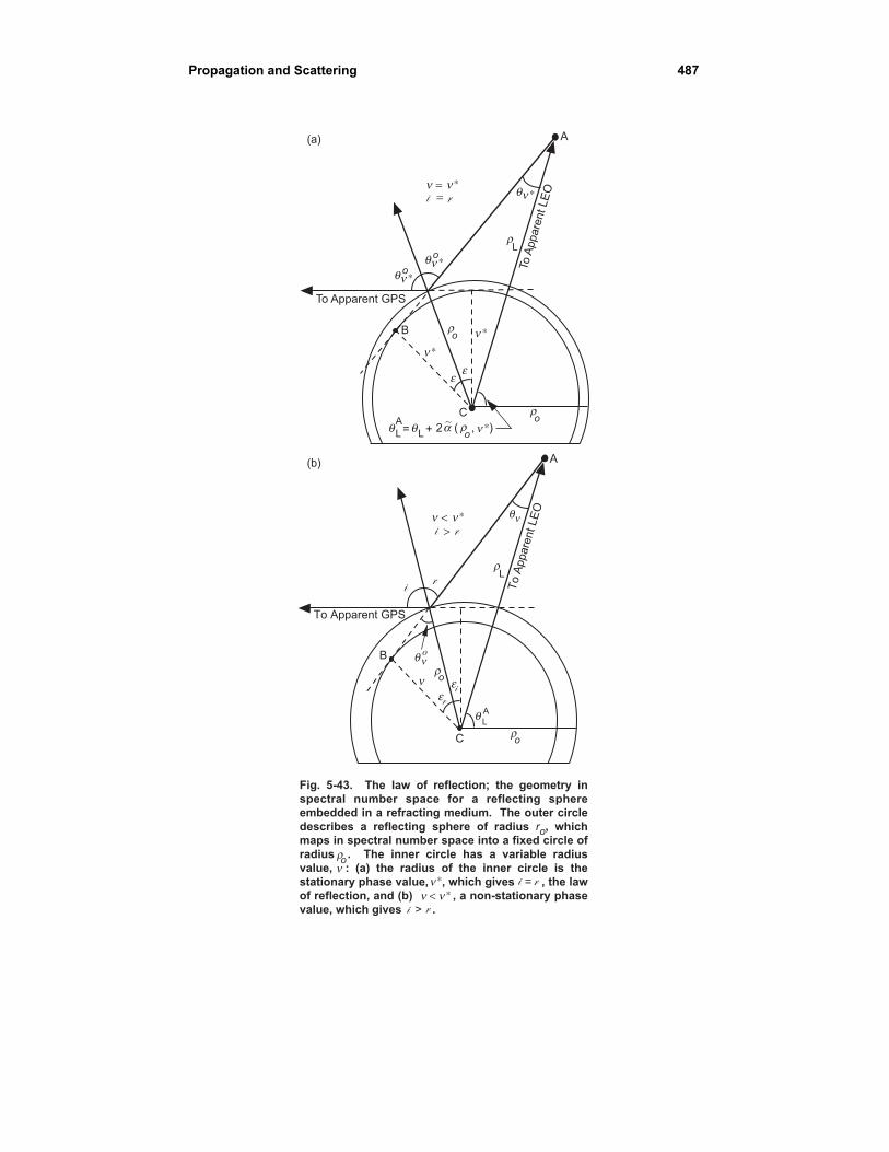
Propagation and Scattering 487
To Apparent GPS
To A
ppare
nt LE
O
n *qL
qL
Aro
2a~
( ),= +
ee
n *
n *
n *q
ro
n *qo
n *qo
ro
B
C
A(a)
rL
n n<
<
*
i r
(b)
ro
ro
rL
To A
ppare
nt LE
O
To Apparent GPS
A
C
B
n
Lq
A
qn
qno
i r
er
ei
Fig. 5-43. The law of reflection; the geometry in
spectral number space for a reflecting sphere
embedded in a refracting medium. The outer circle
describes a reflecting sphere of radius ro, which
maps in spectral number space into a fixed circle of
radius . The inner circle has a variable radius
value, : (a) the radius of the inner circle is the
stationary phase value, , which gives = , the law
of reflection, and (b) , a non-stationary phase
value, which gives > .
ro
n*
< nn *
n
i
i
r
r
n n=
=
*
i r

488 Chapter 5
ε π θθ θ θ θ
θ
θ θ α ρ ν θ
νρ ρ
ρ= − =−
+−( )
+ ⋅ ⋅ ⋅
= − + ( ) −
2 2 16
212
2
*L L
L
tan
˙ ˜ , tan*
oA A
oo o o
o o
o
N
(5.14-27)
For the exponential refractivity model given in Eq. (5.8-2) and from theresulting bending-angle expression given in Eq. (5.8-3), we have
ε θ θ α ρ ρ ρ θ θ θ˙ ˜ ( , ) tanLL= − + − −( ) −o
o oo o
o o oN
HN
2 212
(5.14-28)
Thus, the refractive bending (for a negative refractivity gradient, i.e.,˜ , *α ρ νo( ) > 0) acts to increase the counterclockwise rotation of the reflection
point. This is qualitatively indicated in Fig. 5-36. For sea-level conditions andfor θ θL mrad− =o 10 , the third and fourth terms on the RHS of Eq. (5.14-28)provide a correction of about 10 percent.
For a backward reflection case, that is, when θ πL /> 2, the incoming
spectral coefficients al− ( )Lρ also would have to be taken into account. When
θ πL />> 2, this geometry would correspond more closely to a near-verticalreflection geometry than to the near-grazing one discussed here.
References
[1] C. Chapman and J. Orcutt, “The Computation of Body Wave SyntheticSeismograms in Laterally Homogeneous Media,” Reviews of Geophysics,vol. 23, no. 2, pp. 105–163, 1985.
[2] G. Mie, “Beiträge zur Optik Truber Medien Speziell KolliodalerMetallösungen,” Annales de Physique (Leipzig), vol. 25, pp. 377–452,1908.
[3] M. Born and E. Wolf, Principles of Optics: Electromagnetic Theory ofPropagation, Interference, and Diffraction of Light, 6th ed., New York,New York: Pergamon Press, 1980.
[4] J. Jackson, Classical Electrodynamics, 2nd ed., Oxford, United Kingdom:J. Wiley & Sons, Inc., 1975.
[5] T. Eckersley and G. Millington, “Application of the Phase IntegralMethod to the Analysis of the Diffraction and Reflection of WirelessWaves Round the Earth.” Philos. Trans., vol. 237, pp. 273–309, 1938.
[6] J. Mathews and R. Walker, Mathematical Methods of Physics, MenloPark, California: The Benjamin/Cummings Publishing Co., 1970.

Propagation and Scattering 489
[7] M. Levy, Parabolic Equation Methods for Electromagnetic WavePropagation, London, United Kingdom: The Institution for ElectricalEngineers, 2000.
[8] M. Abramowitz and I. Stegun, eds., Handbook of MathematicalFunctions With Formulas, Graphs, and Mathematical Tables, U.S.Department of Commerce, National Bureau of Standards, U.S.Government Printing Office, Washington, D.C., 1964.
[9] A. Pavelyev, A. Zakharov, A. Kucherjavenkov, E. Molotov, I. Siderenko,I. Kucherjavenkova, and D. Pavelyev, “Propagation of Radio WavesReflected from Earth’s Surface at Grazing Angles between a Low-OrbitSpace Station and a Geostationary Satellite,” Journal of CommunicationsTechnology and Electronics, vol. 42, no. 1, pp. 51–57, 1997.
[10] G. Beyerle, K. Hocke, J. Wickert, T. Schmidt, C. Marquardt, and Ch.Reigber, “GPS Radio Occultations with CHAMP: A Radio HolographicAnalysis of GPS Signal Propagation in the Troposphere and SurfaceReflections,” Journal of Geophysical Research, vol. 107, no. D24,10.1029/ 2001JD001402, 2002.