Embed Size (px)
Citation preview
1 | P a g e
CHAPTER 5
POVERTY ALLEVIATION IN INDIA: AN APPLICATION OF SIMULTANEOUS
EQUATION MODELS ON RURAL POPULATION UNDER POVERTY LINE
FROM OFFICIAL STATISTICS – THE WORLD BANK
5.1 INTRODUCTION
Poverty in rural India has declined substantially in recent decades. By 1990,
about 34 percent of the rural population was poor (Figure 5.1). The percentage
of poor increased again to about 40 percent of the population when policy
reforms were implemented in the early 1990s, but it now seems to be declining
again. The steady decline in poverty from the mid- 1960s to the early 1980s
was strongly associated with agricultural growth, particularly the Green
Revolution. Since then, the causes for the decline seem to have become more
complex. Nonfarm wages and employment now play a much larger role in
reducing poverty, and these are less driven by agricultural growth than before.
The government spending on rural poverty and employment programs has
increased substantially in recent years, and this has directly benefited the rural
poor. The purpose of this research is to investigate the causes of the decline in
rural poverty in India and particularly to determine the role that government
investments have played. Government spending can have direct and indirect
effects on poverty. The direct effects are the benefits the poor receive from
expenditures on employment and welfare programs such as the Integrated
Rural Development Program and from various rural employment schemes that
are directly targeted to the poor during drought years. The indirect effects arise
2 | P a g e
when government investments in rural infrastructure, agricultural research, and
the health and education of rural people stimulate agricultural and non
agricultural growth, leading to greater employment and income-earning
opportunities for the poor and to cheaper food. In this study, the effectiveness
of different types of government expenditures in contributing to poverty
alleviation is quantified. Such information can assist policymakers in targeting
their investments more effectively to reduce poverty. More efficient targeting
has become increasingly important in an era of macroeconomic reforms in
which the government is under pressure to reduce its total budget. An
econometric model is formulated and estimated that permits calculation of the
number of poor people raised above the poverty line for each additional million
rupees spent on different expenditure items. But targeting government
expenditures simply to reduce poverty is not sufficient. Government
expenditures also need to stimulate economic growth to help generate the
resources required for future government expenditures. Growth is the only sure
way of providing a permanent solution to the poverty problem and of
increasing the overall welfare of rural people. This model is therefore
formulated to measure the impact on growth as well as poverty of different
items of government expenditure. The model makes it possible not only to rank
different types of investment in terms of their effects on growth and poverty,
but also to quantify any trade-offs or complementarities that may arise in the
achievement of these two goals.
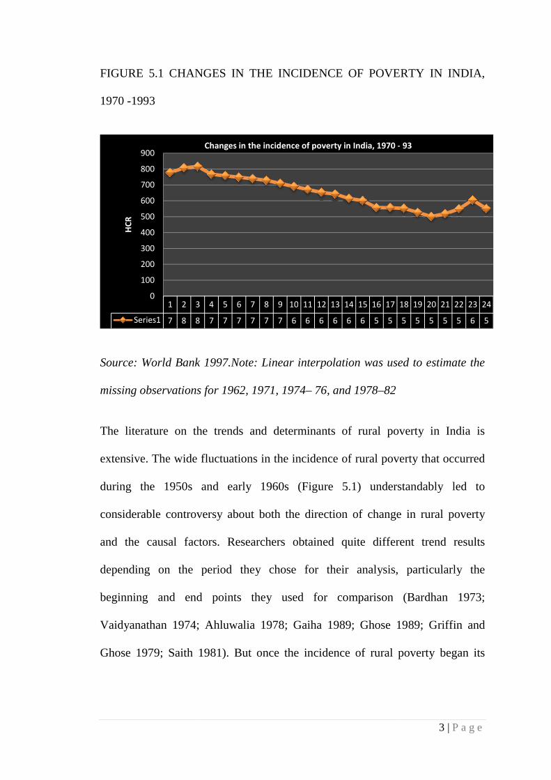
FIGURE 5.1 CHANGES IN THE INCIDENCE OF POVERTY IN INDIA,
1970 -1993
Source: World Bank 1997.Note: Linear interpolation was used to estimate the
missing observations for 1962, 1971, 1974
The literature on the trends and determinants of rural poverty in India is
extensive. The wide fluctuations in the incidence of rural p
during the 1950s and early 1960s (Figure
considerable controversy about both the direction of change in rural poverty
and the causal factors. Researchers obtained quite different trend results
depending on the period they chose for their analysis, particularly the
beginning and end points they used for comparison (Bardhan 1973;
Vaidyanathan 1974; Ahluwalia 1978; Gaiha 1989; Ghose 1989; Griffin and
Ghose 1979; Saith 1981). But once the incidence of rural povert
1 2 3
Series1 7 8 8
0
100
200
300
400
500
600
700
800
900
HC
R
CHANGES IN THE INCIDENCE OF POVERTY IN INDIA,
Bank 1997.Note: Linear interpolation was used to estimate the
missing observations for 1962, 1971, 1974– 76, and 1978–82
The literature on the trends and determinants of rural poverty in India is
extensive. The wide fluctuations in the incidence of rural poverty that occurred
during the 1950s and early 1960s (Figure 5.1) understandably led to
considerable controversy about both the direction of change in rural poverty
and the causal factors. Researchers obtained quite different trend results
e period they chose for their analysis, particularly the
beginning and end points they used for comparison (Bardhan 1973;
Vaidyanathan 1974; Ahluwalia 1978; Gaiha 1989; Ghose 1989; Griffin and
Ghose 1979; Saith 1981). But once the incidence of rural povert
3 4 5 6 7 8 9 10 11 12 13 14 15 16 17
8 7 7 7 7 7 7 6 6 6 6 6 6 5 5
Changes in the incidence of poverty in India, 1970 -
3 | P a g e
CHANGES IN THE INCIDENCE OF POVERTY IN INDIA,
Bank 1997.Note: Linear interpolation was used to estimate the
The literature on the trends and determinants of rural poverty in India is
overty that occurred
) understandably led to
considerable controversy about both the direction of change in rural poverty
and the causal factors. Researchers obtained quite different trend results
e period they chose for their analysis, particularly the
beginning and end points they used for comparison (Bardhan 1973;
Vaidyanathan 1974; Ahluwalia 1978; Gaiha 1989; Ghose 1989; Griffin and
Ghose 1979; Saith 1981). But once the incidence of rural poverty began its
18 19 20 21 22 23 24
5 5 5 5 5 6 5
- 93
4 | P a g e
trend decline in the mid-1960s, a greater consensus began to emerge in the
literature (Ghose 1989; Ravallion and Datt 1995; Ninan 1994).
5.2 GOVERNMENT EXPENDITURE
Government expenditure in India is divided into non development and
development spending, and the latter is further sub divided into spending on
social and economic services. Social services include health, labor, and other
community services, while economic services include such sectors as
agriculture, industry, trade, and transportation. State governments are
responsible for irrigation, power, agriculture, animal husbandry, dairy, soil
conservation, education, health, family planning, cooperatives, rural
development, forests, and more. Local functions such as public order, courts,
and police are also the responsibility of the state governments.
Most expenditure on agriculture and rural areas are undertaken by the state
governments. This includes expenditures financed from the states’ own
revenues, but even the central government’s expenditure on agriculture and
rural development is largely channeled through the state governments.
1. TECHNOLOGY, INFRASTRUCTURE, AND GROWTH
The introduction of new technologies, improved infrastructure (roads and
electrification), and education have all contributed to agricultural growth in
India. This section analyzes these developments and provides a basis for the
analysis in later sections of how these government investments have reduced
rural poverty in directly through improved agricultural productivity.
5 | P a g e
2. TECHNOLOGIES, INFRASTRUCTURE, AND EDUCATION
One of the most significant changes in Indian agriculture in recent decades has
been the wide spread adoption of high- yielding varieties (HYVs). During the
Green Revolution of the 1970s, the crop area planted to HYVs for five major
crops (rice, wheat, maize, sorghum, and pearl millet) increased from less than
17 percent in 1970 to 40 percent in 1980. Even after the Green Revolution had
peaked, the percentage of the crop area planted with HYVs continued to
increase. As with the adoption of HYVs, there seems to be a strong correlation
between poverty and the extent of irrigation among states. Since HYVs
respond well to irrigation and high rates of fertilizer use, lack of irrigation
facilities in these states has hindered more wide spread adoption of HYVs. One
of the greatest achievements in the development of rural India has been the
rapid increase of electrification. Surprisingly, the literacy rate in some well-
developed states such as Andhra Pradesh and Haryana remains below the
national average. Road density in rural India, measured as the length of roads
in kilometers per thousand square kilometers of geographic area, increased
from 2,614 in 1970 to 5,704 in 1995, a growth rate of more than 3 percent a
year. The regional data show that development of road density is highly
correlated with poverty reduction.
3. PRODUCTION AND PRODUCTIVITY GROWTH
As a result of rapid adoption of new technologies and improved rural
infrastructure, agricultural production and factor productivity have both grown
6 | P a g e
rapidly in India. Five major crops (rice, wheat, sorghum, pearl millet, and
maize), 14 minor crops (barley, cotton, groundnut, other grain, other pulses,
potato, rapeseed, mustard, sesame, sugar, tobacco, soybeans, jute, and sun
flower), and 3 major live stock products (milk, meat, and chicken) are included
in this measure of total production. Unlike traditional measures of production
growth, which use constant output prices, the more appropriate TÖRNQVIST-
THEIL index (a discrete approximation to the Divisia index is used. As Richter
(1966) has shown, the Divisia index is desirable because of it’s in variance
property: if nothing real has changed (for example, if the only input quantity
changes involve movements along an unchanged iso - quant), then the index
itself is unchanged (Alston, Norton, and Pardey 1998). The formula for the
index of aggregate production is
ln YIt = ∑i ½(Si,t + Si,t-1) ln (Yi,t /Yi,t-1) (A)
where ln YItis the log of the production index at time t, Si, t and Si, t–1 are
output i’s share in total production value at time t and t–1, respectively, and Yi,
t and Yi, t–1 are quantities of output i at time t and t–1, respectively. Farm
prices are used to calculate the weights of each crop in the value of total
production.
Agricultural production grew slowly in the high- poverty states like Assam and
Bihar, but much faster in the low- poverty states like Andhra Pradesh,
Karnataka, and Punjab. To gain richer insights into the sources and efficiency
of agricultural production growth, a “total” factor productivity index was
calculated. Total factor productivity (TFP) is defined as aggregate output minus
7 | P a g e
aggregate in puts. Again, a TÖRNQVIST-THEIL index is used to aggregate
both in puts and out puts. Specifically,
ln TFPt = ∑i ½(Si,t + Si,t-1) ln (Yi,t /Yi,t-1) - ∑i ½(Wi,t + Wi,t-1) ln (Xi,t /Xi,t-1) (B)
where ln TFPtis the log of the TFP index; Wi, tand Wi, t–1 are cost shares of input
i in total cost at time t and t–1, respectively; and Xi, t and Xi, t–1 are quantities of
input i at time t and t–1, respectively. Five inputs (labor, land, fertilizer,
tractors, and buffalos) are included. Labor in put is measured as the total
number of male and female workers employed in agriculture at the end of each
year; land is measured as gross cropped area; fertilizer input as the total amount
of nitrogen, phosphate, and potassium used; tractor input as the number of four-
wheel tractors; and bullock input as the number of adult bullocks. The wage
rate for agricultural labor is used as the price of labor to aggregate total cost for
labor: the costs of draft animals and machinery are taken directly from the
production cost surveys; and the fertilizer cost is the product of total fertilizer
use and fertilizer price calculated as a weighted average of the prices of
nitrogen, phosphate, and potassium. The land cost is measured as the residual
of total revenue net of measured costs for labor, fertilizer, tractors, and
bullocks. Therefore, the cost share of each input is calculated by its respective
cost divided by total production value..
Since 1990, TFP growth in Indian agriculture has continued to grow but at a
slower rate of 2.29 per cent per year. For the whole period 1970–94, Punjab
and West Bengal had the highest growth rates in TFP, while in Assam, Gujarat,
and Rajasthan, TFP improved only slightly or even declined during this period.
8 | P a g e
The correlation between productivity growth and poverty reduction is stronger
than that between production growth and poverty reduction, suggesting that
productivity growth may be the more important variable to use for explaining
poverty.
4. RURAL EMPLOYMENT AND WAGES
Rural employment in India has undergone several significant changes. Total
rural employment grew very little in the 1970s and even declined in the mid-
1980s. Non agricultural employment has grown faster than agricultural
employment, and growth in non agricultural employment has accelerated in
recent years.
Government investment in roads, power, and rural development may have
contributed to this rapid increase, as will be discussed later. Rural development
investment is specifically targeted by the government to alleviate rural poverty
by generating rural employment.
The level and structure of employment and wages seem to have moved
together. First, there is a clear contrast between the pre- and post- 1987
situation. Agricultural employment actually declined between 1970 and 1987,
while nonfarm employment grew at an increasing rate. The increase in nonfarm
employment coincides with a steady increase in rural wages. The increase in
rural poverty associated with the introduction of the policy reforms may have
induced workers to accept lower productivity jobs. State-level data reveal that
in poor states such as Bihar, Orissa, and Uttar Pradesh, not only is non
9 | P a g e
agricultural employment less important in total rural employment, but the
growth rate is among the lowest of all the states.
5. RURAL POVERTY
The changes in rural poverty since 1951 measured as a head- count ratio. The
head- count ratio is the percentage of the rural population falling below the
poverty line. As discussed earlier, the rapid adoption of HYVs together with
improved irrigation increased agricultural production and productivity growth.
This change in technology was a direct result of increased government
investment in agricultural research and extension, infrastructure, irrigation, and
education. The increase in government investment also improved non
agricultural employment opportunities and wages, contributing directly to
further reductions in rural poverty. The stagnation in agricultural productivity
growth and the increase in rural poverty observed in the early 1990s may have
resulted from reduced government investment in rural areas during this period.
State-level data reveal wide variations in the level of rural poverty and change
in its incidence. The poverty ratios declined at relatively higher rates per year
in Andhra Pradesh, Kerala, Maharashtra, Punjab, Tamil Nadu, and West
Bengal, and at lower rates in Bihar, Haryana, and Rajasthan.
Given the observed diversity in the rates of poverty alleviation across states, it
is important to ask whether there is a relationship between the rates of change
and the initial levels of poverty. Does poverty go down faster in those states
that had less poverty to begin with or in those states that had higher initial
poverty levels? To answer this question, correlation coefficients across the 14
10 | P a g e
states were calculated between the head-count ratios and the annual rates of
change in poverty. The correlations indicate that the relationship between the
level of poverty in 1957 and the percentage change in the level of poverty
during 1957–60 was negative and significant. This means that the biggest
reductions in rural poverty occurred in the poorest states.
5 .3 THEORETICAL FRAMEWORK
Most previous studies of the determinants of rural poverty in India have used a
single equation approach and have tried to explain rural poverty as a function
of explanatory variables like agricultural production, wages, and the price of
food. The conceptual frame work proposed for this analysis is a simultaneous
structural equations system in which many economic variables are endogenous,
and their direct and indirect interactions are explicitly considered in the model.
There are at least three advantages to this approach. First, the simultaneous
system allows us to indigenize many economic variables that are likely to be
generated in the same economic process, therefore, reducing or even
eliminating the bias resulting from the endogeneity of these variables in the
empirical econometric estimation of the various effects. Second, certain
economic variables such as government investments affect poverty through
multiple channels. For example, government investment in roads will not only
reduce rural poverty through improved agricultural productivity, it will also
affect rural poverty through improved wages and nonfarm employment. The
simultaneous equations system will also allow us to estimate these various
direct and in direct effects. Third, it will also enable us to observe where the
11 | P a g e
weak link is in the economic process of productivity growth and poverty
reduction.
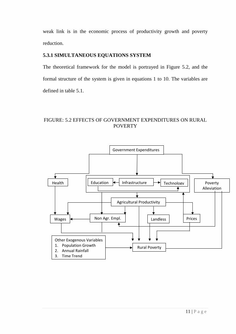
5.3.1 SIMULTANEOUS EQUATIONS SYSTEM
The theoretical framework for the model is portrayed in Figure 5.2, and the
formal structure of the system is given in equations 1 to 10. The variables are
defined in table 5.1.
FIGURE: 5.2 EFFECTS OF GOVERNMENT EXPENDITURES ON RURAL POVERTY
Health Education Technology Infrastructure Poverty
Alleviation
Wages Prices Non Agr. Empl. Landless
Agricultural Productivity
Other Exogenous Variables
1. Population Growth
2. Annual Rainfall
3. Time Trend
Rural Poverty
Government Expenditures
12 | P a g e
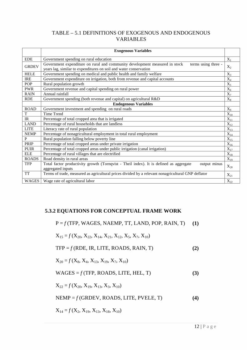
TABLE – 5.1 DEFINITIONS OF EXOGENOUS AND ENDOGENOUS VARIABLES
Exogenous Variables
EDE Government spending on rural education X1
GRDEV Government expenditure on rural and community development measured in stock terms using three - years lag, similar to expenditures on soil and water conservation
X2
HELE Government spending on medical and public health and family welfare X3 IRE Government expenditure on irrigation, both from revenue and capital accounts X4 POP Rural population growth X5 PWR Government revenue and capital spending on rural power X6 RAIN Annual rainfall X7 RDE Government spending (both revenue and capital) on agricultural R&D X8 Endogenous Variables ROAD Government investment and spending on rural roads X9 T Time Trend X10 IR Percentage of total cropped area that is irrigated X11 LAND Percentage of rural households that are landless X12 LITE Literacy rate of rural population X13 NEMP Percentage of nonagricultural employment in total rural employment X14 P Rural population falling below poverty line X15 PRIP Percentage of total cropped areas under private irrigation X16 PUIR Percentage of total cropped areas under public irrigation (canal irrigation) X17 ELE Percentage of rural villages that are electrified X18 ROADS Road density in rural areas X19 TFP Total factor productivity growth (Tornqvist - Theil index). It is defined as aggregate output minus
aggregated inputs X20
TT Terms of trade, measured as agricultural prices divided by a relevant nonagricultural GNP deflator X21
WAGES Wage rate of agricultural labor X22
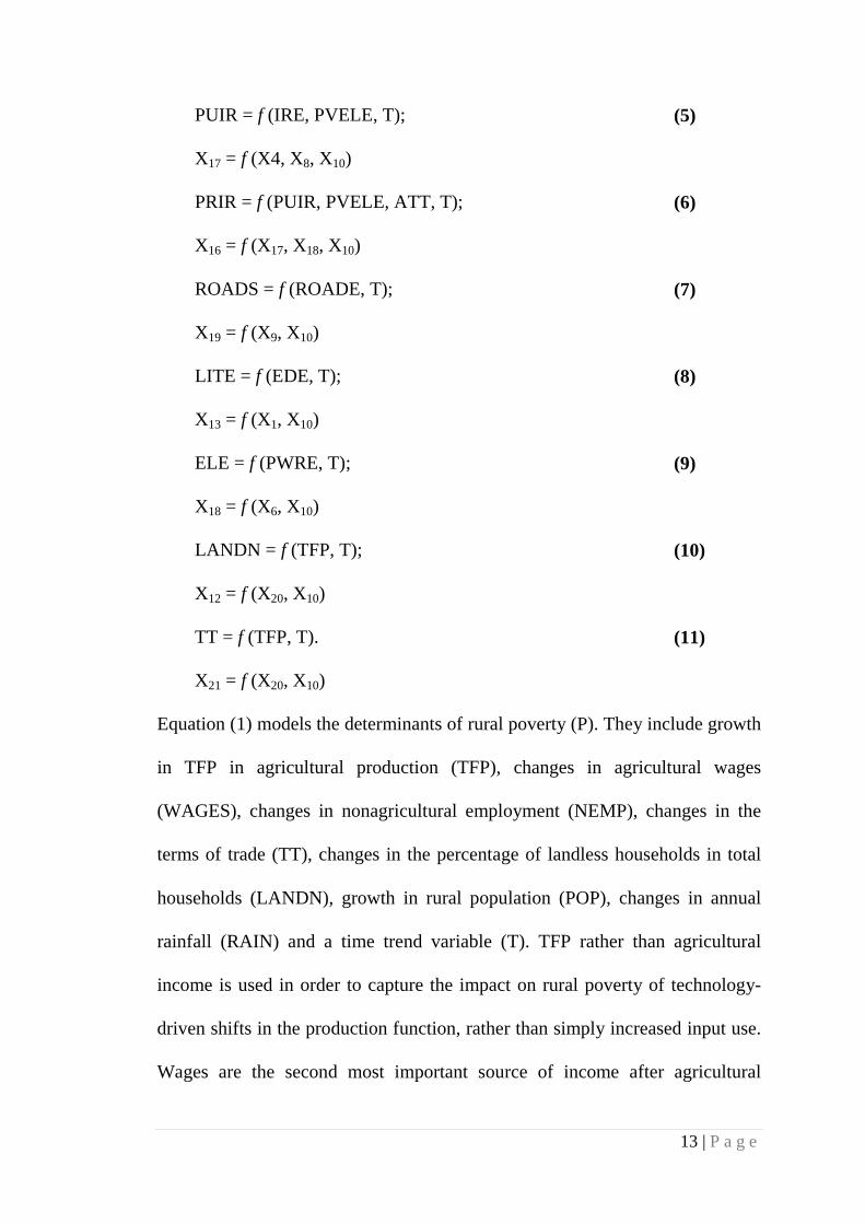
5.3.2 EQUATIONS FOR CONCEPTUAL FRAME WORK
P = f (TFP, WAGES, NAEMP, TT, LAND, POP, RAIN, T) (1)
X15 = f (X20, X22, X14, X21, X12, X5, X7, X10)
TFP = f (RDE, IR, LITE, ROADS, RAIN, T) (2)
X20 = f (X8, X4, X13, X19, X7, X10)
WAGES = f (TFP, ROADS, LITE, HEL, T) (3)
X22 = f (X20, X19, X13, X3, X10)
NEMP = f (GRDEV, ROADS, LITE, PVELE, T) (4)
X14 = f (X2, X19, X13, X18, X10)
13 | P a g e
PUIR = f (IRE, PVELE, T); (5)
X17 = f (X4, X8, X10)
PRIR = f (PUIR, PVELE, ATT, T); (6)
X16 = f (X17, X18, X10)
ROADS = f (ROADE, T); (7)
X19 = f (X9, X10)
LITE = f (EDE, T); (8)
X13 = f (X1, X10)
ELE = f (PWRE, T); (9)
X18 = f (X6, X10)
LANDN = f (TFP, T); (10)
X12 = f (X20, X10)
TT = f (TFP, T). (11)
X21 = f (X20, X10)
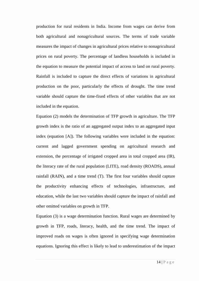
Equation (1) models the determinants of rural poverty (P). They include growth
in TFP in agricultural production (TFP), changes in agricultural wages
(WAGES), changes in nonagricultural employment (NEMP), changes in the
terms of trade (TT), changes in the percentage of landless households in total
households (LANDN), growth in rural population (POP), changes in annual
rainfall (RAIN) and a time trend variable (T). TFP rather than agricultural
income is used in order to capture the impact on rural poverty of technology-
driven shifts in the production function, rather than simply increased input use.
Wages are the second most important source of income after agricultural
14 | P a g e
production for rural residents in India. Income from wages can derive from
both agricultural and nonagricultural sources. The terms of trade variable
measures the impact of changes in agricultural prices relative to nonagricultural
prices on rural poverty. The percentage of landless households is included in
the equation to measure the potential impact of access to land on rural poverty.
Rainfall is included to capture the direct effects of variations in agricultural
production on the poor, particularly the effects of drought. The time trend
variable should capture the time-fixed effects of other variables that are not
included in the equation.
Equation (2) models the determination of TFP growth in agriculture. The TFP
growth index is the ratio of an aggregated output index to an aggregated input
index (equation [A]). The following variables were included in the equation:
current and lagged government spending on agricultural research and
extension, the percentage of irrigated cropped area in total cropped area (IR),
the literacy rate of the rural population (LITE), road density (ROADS), annual
rainfall (RAIN), and a time trend (T). The first four variables should capture
the productivity enhancing effects of technologies, infrastructure, and
education, while the last two variables should capture the impact of rainfall and
other omitted variables on growth in TFP.
Equation (3) is a wage determination function. Rural wages are determined by
growth in TFP, roads, literacy, health, and the time trend. The impact of
improved roads on wages is often ignored in specifying wage determination
equations. Ignoring this effect is likely to lead to underestimation of the impact
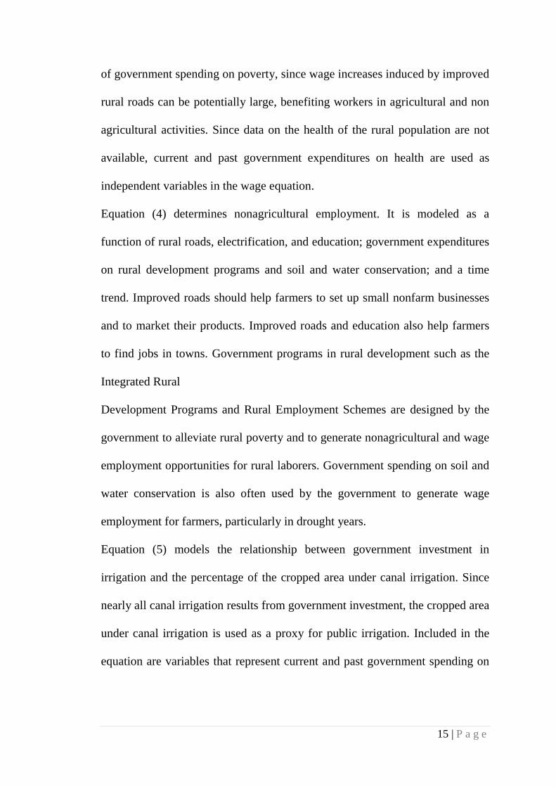
15 | P a g e
of government spending on poverty, since wage increases induced by improved
rural roads can be potentially large, benefiting workers in agricultural and non
agricultural activities. Since data on the health of the rural population are not
available, current and past government expenditures on health are used as
independent variables in the wage equation.
Equation (4) determines nonagricultural employment. It is modeled as a
function of rural roads, electrification, and education; government expenditures
on rural development programs and soil and water conservation; and a time
trend. Improved roads should help farmers to set up small nonfarm businesses
and to market their products. Improved roads and education also help farmers
to find jobs in towns. Government programs in rural development such as the
Integrated Rural
Development Programs and Rural Employment Schemes are designed by the
government to alleviate rural poverty and to generate nonagricultural and wage
employment opportunities for rural laborers. Government spending on soil and
water conservation is also often used by the government to generate wage
employment for farmers, particularly in drought years.
Equation (5) models the relationship between government investment in
irrigation and the percentage of the cropped area under canal irrigation. Since
nearly all canal irrigation results from government investment, the cropped area
under canal irrigation is used as a proxy for public irrigation. Included in the
equation are variables that represent current and past government spending on
16 | P a g e
irrigation, the extent of rural electrification (the percentage of villages that have
been electrified), a lagged terms-of-trade variable, and a time trend.
Equation (6) models the determinants of private irrigation. It is hypothesized
that canal irrigation supported by the government is often a precursor to private
irrigation, because it increases the economic returns to investments in wells and
pump sets (by raising the groundwater level). Private irrigation is defined as the
percentage of the cropped area under wells and tube wells, which are mostly
the result of farmers’ private initiatives. Other determinants of private irrigation
investment in equation (6) are rural electrification, the terms of trade, and the
time trend.
Equations (7), (8), and (9) model the relationships between lagged government
expenditures on roads, education, and rural electrification and the available
stock of these variables. In equation (7), the stock of roads (measured in
density form) is specified as a lagged function of government expenditures on
roads and time trend T. Similarly, the literacy rate at any point in time is a
lagged function of past government spending on education and time T
(equation [8]). The percentage of villages that are electrified depends on past
government spending on power and the time event (equation [9]).
Equation (10) models the effect of productivity growth on access to land
(measured as the incidence of landlessness). It has often been argued that
improved productivity as a result of technological change and infrastructure
improvements has worsened equity problems in rural areas. Endogenizing
access to land in the model should capture these effects.
17 | P a g e
Equation (11) determines the terms of trade. Growth in TFP in the state and at
the national level increases the aggregate supply of agricultural products, and
therefore reduces agricultural prices. Lower prices will help the poor if they are
net buyers of grains. The inclusion of national TFP growth will help to reduce
any upward bias in the estimation of the poverty alleviation effects of
government spending within each state, since TFP growth in other states will
also contribute to lower food prices through the national market. A world price
index of rice, wheat, and corn is included in the equation to capture the impact
of international markets on domestic agricultural prices. Some demand-side
variables were also included in an earlier version of the equation, such as
population and income growth, but they were not significant and were dropped
from the equation. Part of the effects of these omitted variables is captured by
the time trend variable.
5.4 MARGINAL EFFECTS OF GOVERNMENT EXPENDITURES ON
POVERTY
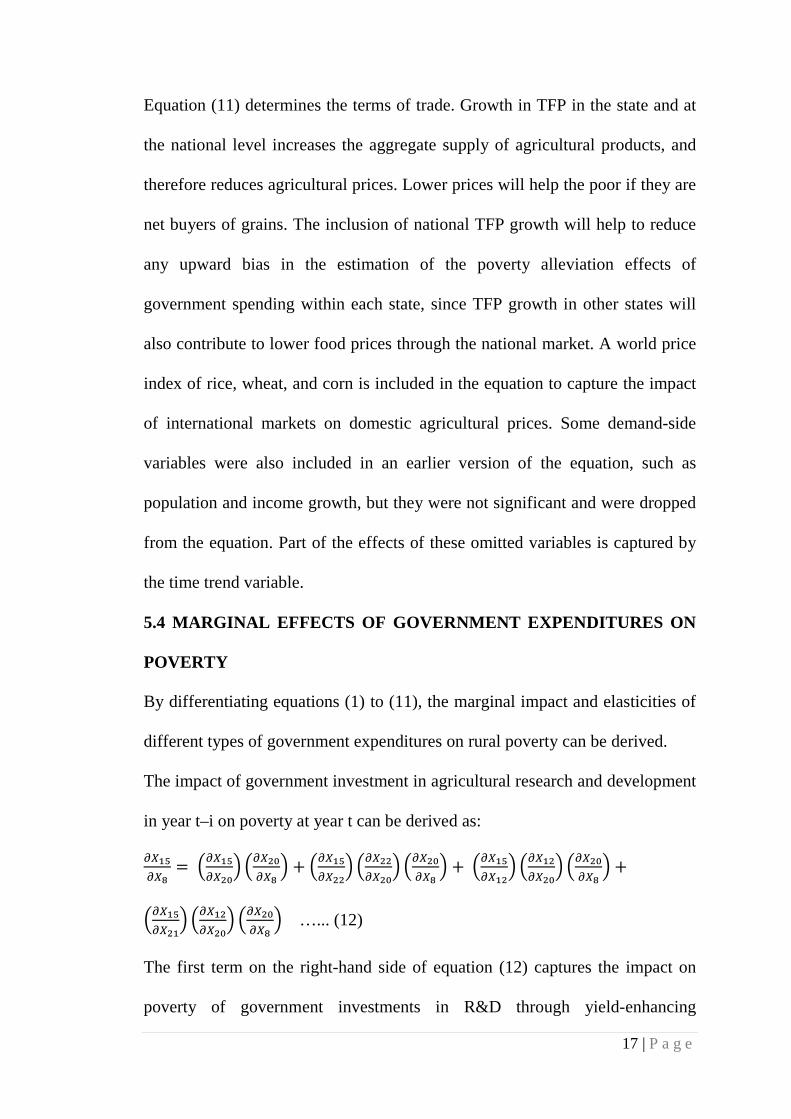
By differentiating equations (1) to (11), the marginal impact and elasticities of
different types of government expenditures on rural poverty can be derived.
The impact of government investment in agricultural research and development
in year t–i on poverty at year t can be derived as:
�������
� �������
� ������
� � �������
� �����
� ������
� � ��������
� ������
� ������
� �
��������
� ������
� ������
� …... (12)
The first term on the right-hand side of equation (12) captures the impact on
poverty of government investments in R&D through yield-enhancing
18 | P a g e
technologies such as improved varieties and therefore TFP. Increased TFP also
affects poverty through changes in wages, access to land, and relative prices,
which are captured in the remaining terms of the right-hand side of the
equation. By aggregating the total effects of all past government expenditures
over the lag period, the sum of marginal effects is obtained for any particular
year. The impact of government investment in irrigation in year t–j on poverty
in year t is derived as:
������
�
�������
� �������
� �������
� � �������
� �����
� �������
� �������
� �
��������
� ������
� �������
� �������
� � ��������
� ������
� �������
� �������
� �
�������
� �������
� ���������
� �������
�+�������
� �����
� �������
� ���������
� �������
�+
��������
� ������
� �������
� ���������
� �������
� � ��������
� ������
� �������
� ���������
� �������
� … �13�
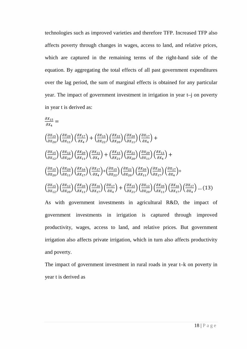
As with government investments in agricultural R&D, the impact of
government investments in irrigation is captured through improved
productivity, wages, access to land, and relative prices. But government
irrigation also affects private irrigation, which in turn also affects productivity
and poverty.
The impact of government investment in rural roads in year t–k on poverty in
year t is derived as
19 | P a g e
�������
� ���������
� ���������
� ��������
� � ���������
� ���������
� ���������
� ��������
�
� ���������
� ���������
� ���������
� ��������
�
� ���������
� ���������
� ���������
� ��������
� � ������� � �����
����� �����
����
� ���������
� ���������
� ��������
� … �14�
The first term on the right-hand side of equation (14) measures the direct
effects of improved productivity on poverty attribuTable to a greater road
density. Terms 2, 3, and 4 are the indirect effects of improved productivity
through changes in wages, access to land, and prices. Term 5 captures the
effects on poverty of greater non agricultural employment opportunities. The
sixth term of the equation is the impact of improved agricultural wages arising
from government investment in roads.
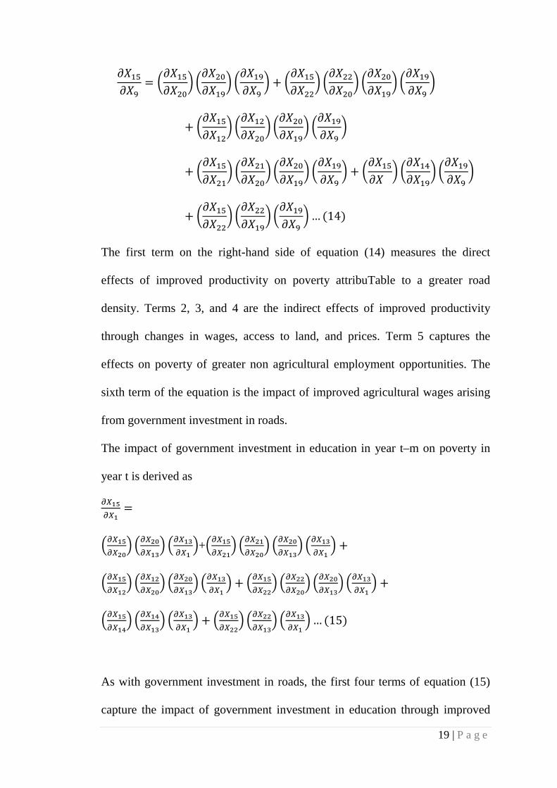
The impact of government investment in education in year t–m on poverty in
year t is derived as
�������
�
�������
� ������
� ���� ���
�+��������
� ������
� ������
� ���� ���
� �
��������
� ������
� ������
� ���� ���
� � �������
� �����
� ������
� ���� ���
� �
��������
� ���� ���
� ���� ���
� � �������
� ������
� ���� ���
� … �15�
As with government investment in roads, the first four terms of equation (15)
capture the impact of government investment in education through improved
20 | P a g e
agricultural productivity. Terms 5 and 6 capture the impact of government
investments in education on poverty through improved nonfarm employment
opportunities and changes in rural wages.
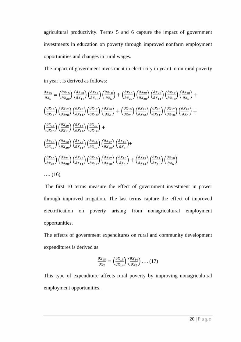
The impact of government investment in electricity in year t–n on rural poverty
in year t is derived as follows:
�������
� �������
� �������
� ���������
� ��������
� � �������
� �����
� �������
� ���������
� ��������
� �
��������
� ������
� �������
� ���������
� ��������
� � ��������
� ������
� �������
� ���������
� ��������
� �
�������
� �������
� ���������
� ���������
� �
��������
� ������
� �������
� ���������
� ���������
� ��������
�+
��������
� ������
� �������
� ���������
� ���������
� ��������
� � ��������
� ���� ����
� ��������
�
…. (16)
The first 10 terms measure the effect of government investment in power
through improved irrigation. The last terms capture the effect of improved
electrification on poverty arising from nonagricultural employment
opportunities.
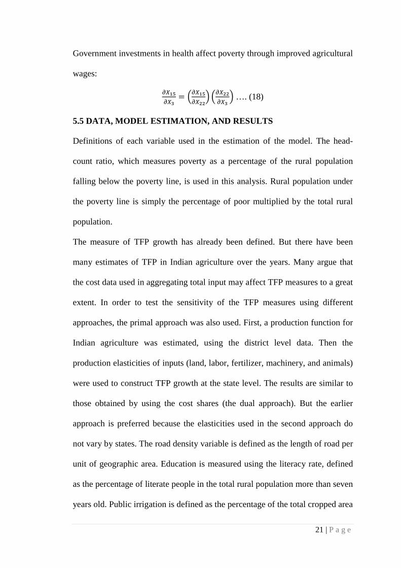
The effects of government expenditures on rural and community development
expenditures is derived as
������
� ��������
� ���� ��
� …. (17)
This type of expenditure affects rural poverty by improving nonagricultural
employment opportunities.
21 | P a g e
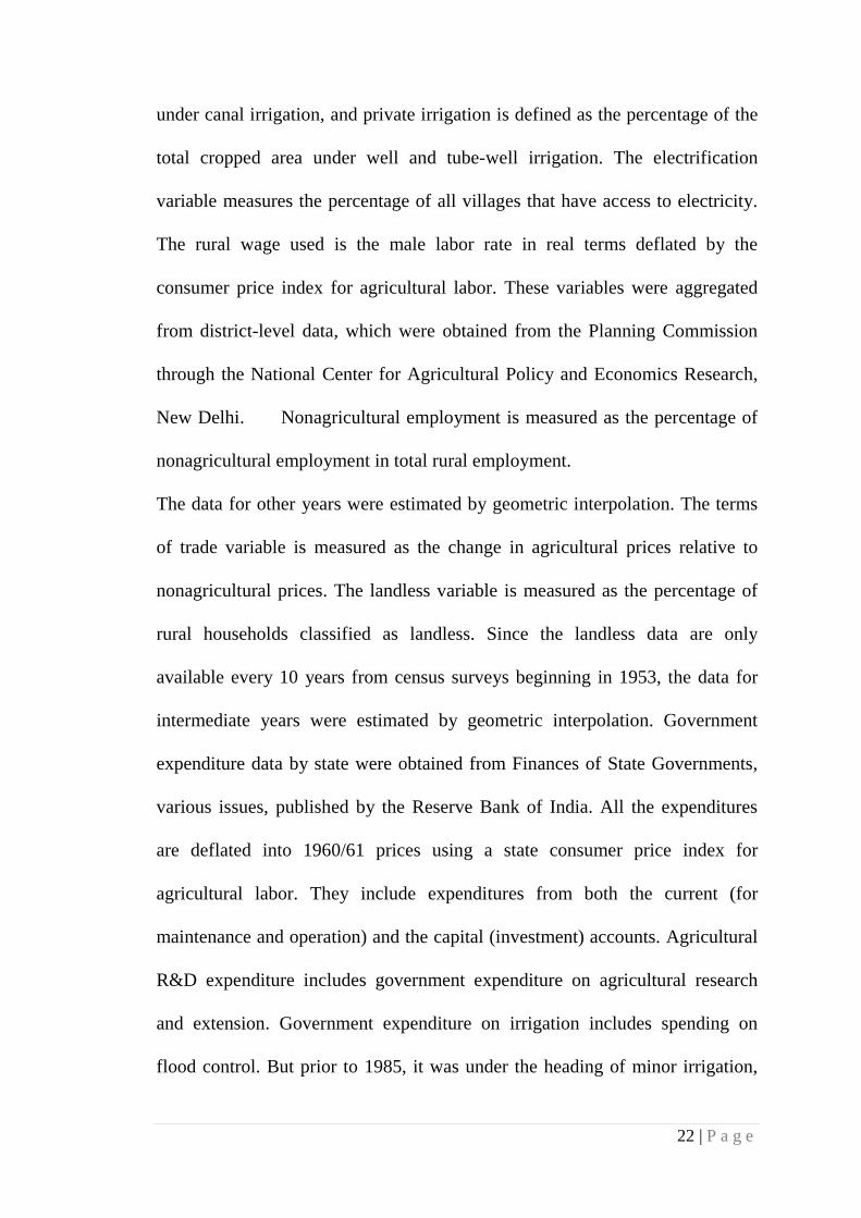
Government investments in health affect poverty through improved agricultural
wages:
������
� �������
� �����
� …. (18)
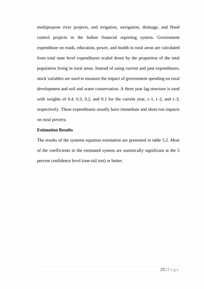
5.5 DATA, MODEL ESTIMATION, AND RESULTS
Definitions of each variable used in the estimation of the model. The head-
count ratio, which measures poverty as a percentage of the rural population
falling below the poverty line, is used in this analysis. Rural population under
the poverty line is simply the percentage of poor multiplied by the total rural
population.
The measure of TFP growth has already been defined. But there have been
many estimates of TFP in Indian agriculture over the years. Many argue that
the cost data used in aggregating total input may affect TFP measures to a great
extent. In order to test the sensitivity of the TFP measures using different
approaches, the primal approach was also used. First, a production function for
Indian agriculture was estimated, using the district level data. Then the
production elasticities of inputs (land, labor, fertilizer, machinery, and animals)
were used to construct TFP growth at the state level. The results are similar to
those obtained by using the cost shares (the dual approach). But the earlier
approach is preferred because the elasticities used in the second approach do
not vary by states. The road density variable is defined as the length of road per
unit of geographic area. Education is measured using the literacy rate, defined
as the percentage of literate people in the total rural population more than seven
years old. Public irrigation is defined as the percentage of the total cropped area
22 | P a g e
under canal irrigation, and private irrigation is defined as the percentage of the
total cropped area under well and tube-well irrigation. The electrification
variable measures the percentage of all villages that have access to electricity.
The rural wage used is the male labor rate in real terms deflated by the
consumer price index for agricultural labor. These variables were aggregated
from district-level data, which were obtained from the Planning Commission
through the National Center for Agricultural Policy and Economics Research,
New Delhi. Nonagricultural employment is measured as the percentage of
nonagricultural employment in total rural employment.
The data for other years were estimated by geometric interpolation. The terms
of trade variable is measured as the change in agricultural prices relative to
nonagricultural prices. The landless variable is measured as the percentage of
rural households classified as landless. Since the landless data are only
available every 10 years from census surveys beginning in 1953, the data for
intermediate years were estimated by geometric interpolation. Government
expenditure data by state were obtained from Finances of State Governments,
various issues, published by the Reserve Bank of India. All the expenditures
are deflated into 1960/61 prices using a state consumer price index for
agricultural labor. They include expenditures from both the current (for
maintenance and operation) and the capital (investment) accounts. Agricultural
R&D expenditure includes government expenditure on agricultural research
and extension. Government expenditure on irrigation includes spending on
flood control. But prior to 1985, it was under the heading of minor irrigation,
23 | P a g e
multipurpose river projects, and irrigation, navigation, drainage, and flood
control projects in the Indian financial reporting system. Government
expenditure on roads, education, power, and health in rural areas are calculated
from total state level expenditures scaled down by the proportion of the total
population living in rural areas. Instead of using current and past expenditures,
stock variables are used to measure the impact of government spending on rural
development and soil and water conservation. A three year lag structure is used
with weights of 0.4, 0.3, 0.2, and 0.1 for the current year, t–1, t–2, and t–3,
respectively. These expenditures usually have immediate and short-run impacts
on rural poverty.
Estimation Results
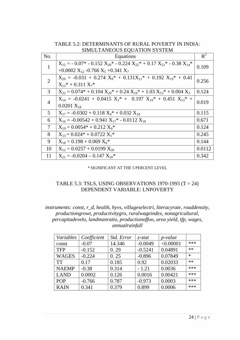
The results of the systems equation estimation are presented in table 5.2. Most
of the coefficients in the estimated system are statistically significant at the 5
percent confidence level (one-tail test) or better.
24 | P a g e
TABLE 5.2: DETERMINANTS OF RURAL POVERTY IN INDIA: SIMULTANEOUS EQUATION SYSTEM
No. Equations R2
1 X15 = - 0.07* - 0.152 X20* - 0.224 X22* + 0.17 X21* - 0.38 X14* +0.0002 X12 -0.766 X5 +0.341 X7
0.109
2 X20 = -0.031 + 0.274 X8* + 0.131X11* + 0.192 X19* + 0.41 X13* + 0.311 X7*
0.256
3 X22 = 0.074* + 0.104 X20* + 0.24 X19* + 1.03 X13* + 0.004 X3 0.124
4 X14 = -0.0241 + 0.0415 X2* + 0.197 X19* + 0.451 X13* + 0.0201 X18
0.019
5 X17 = -0.0302 + 0.118 X4* + 0.032 X18 0.115 6 X16 = -0.00542 + 0.941 X17* - 0.0112 X18 0.671 7 X19 = 0.0054* + 0.212 X9* 0.124 8 X13 = 0.024* + 0.0722 X1* 0.245 9 X18 = 0.198 + 0.069 X6* 0.144 10 X12 = 0.0257 + 0.0199 X20 0.0112 11 X21 = -0.0204 – 0.147 X20* 0.342
* SIGNIFICANT AT THE 5 PERCENT LEVEL
TABLE 5.3: TSLS, USING OBSERVATIONS 1970-1993 (T = 24) DEPENDENT VARIABLE: LNPOVERTY
instruments: const, r_d, health, hyvs, villageselectri, literacyrate, roaddensity, productiongrowt, productivitygro, ruralwageindex, nonagricultural,
percapitadevelo, landmanratio, productionoffoo, area yield, tfp, wages, annualrainfall
Variables Coefficient Std. Error z-stat p-value const -0.07 14.346 -0.0049 <0.00001 *** TFP -0.152 0. 29 -0.5241 0.04891 ** WAGES -0.224 0. 25 -0.896 0.07849 * TT 0.17 0.185 0.92 0.02033 ** NAEMP -0.38 0.314 - 1.21 0.0036 *** LAND 0.0002 0.126 0.0016 0.00421 *** POP -0.766 0.787 -0.973 0.0003 *** RAIN 0.341 0.379 0.899 0.0006 ***
25 | P a g e
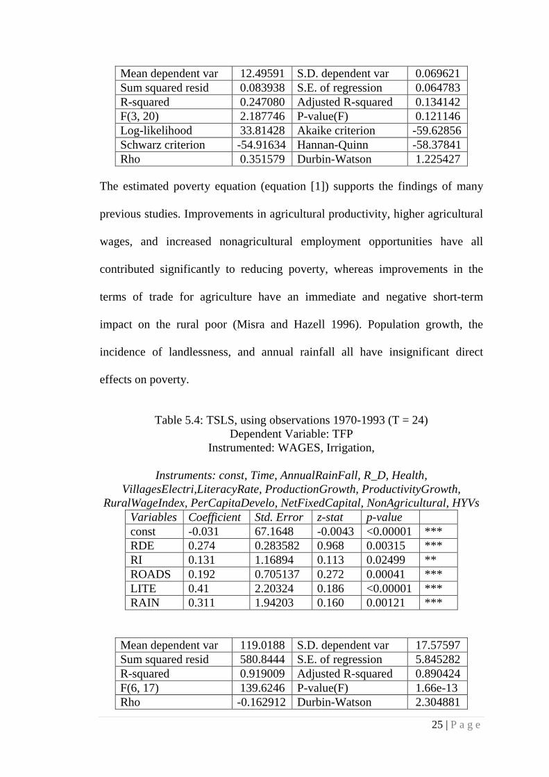
Mean dependent var 12.49591 S.D. dependent var 0.069621 Sum squared resid 0.083938 S.E. of regression 0.064783 R-squared 0.247080 Adjusted R-squared 0.134142 F(3, 20) 2.187746 P-value(F) 0.121146 Log-likelihood 33.81428 Akaike criterion -59.62856 Schwarz criterion -54.91634 Hannan-Quinn -58.37841 Rho 0.351579 Durbin-Watson 1.225427
The estimated poverty equation (equation [1]) supports the findings of many
previous studies. Improvements in agricultural productivity, higher agricultural
wages, and increased nonagricultural employment opportunities have all
contributed significantly to reducing poverty, whereas improvements in the
terms of trade for agriculture have an immediate and negative short-term
impact on the rural poor (Misra and Hazell 1996). Population growth, the
incidence of landlessness, and annual rainfall all have insignificant direct
effects on poverty.
Table 5.4: TSLS, using observations 1970-1993 (T = 24) Dependent Variable: TFP
Instrumented: WAGES, Irrigation,
Instruments: const, Time, AnnualRainFall, R_D, Health, VillagesElectri,LiteracyRate, ProductionGrowth, ProductivityGrowth,
RuralWageIndex, PerCapitaDevelo, NetFixedCapital, NonAgricultural, HYVs Variables Coefficient Std. Error z-stat p-value const -0.031 67.1648 -0.0043 <0.00001 *** RDE 0.274 0.283582 0.968 0.00315 *** RI 0.131 1.16894 0.113 0.02499 ** ROADS 0.192 0.705137 0.272 0.00041 *** LITE 0.41 2.20324 0.186 <0.00001 *** RAIN 0.311 1.94203 0.160 0.00121 ***
Mean dependent var 119.0188 S.D. dependent var 17.57597 Sum squared resid 580.8444 S.E. of regression 5.845282 R-squared 0.919009 Adjusted R-squared 0.890424 F(6, 17) 139.6246 P-value(F) 1.66e-13 Rho -0.162912 Durbin-Watson 2.304881
26 | P a g e
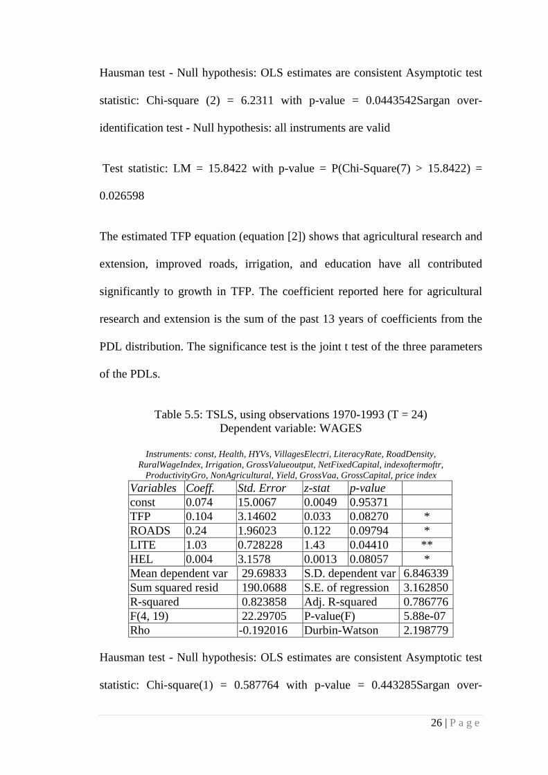
Hausman test - Null hypothesis: OLS estimates are consistent Asymptotic test
statistic: Chi-square (2) = 6.2311 with p-value = 0.0443542Sargan over-
identification test - Null hypothesis: all instruments are valid
Test statistic: LM = 15.8422 with p-value = P(Chi-Square(7) > 15.8422) =
0.026598
The estimated TFP equation (equation [2]) shows that agricultural research and
extension, improved roads, irrigation, and education have all contributed
significantly to growth in TFP. The coefficient reported here for agricultural
research and extension is the sum of the past 13 years of coefficients from the
PDL distribution. The significance test is the joint t test of the three parameters
of the PDLs.
Table 5.5: TSLS, using observations 1970-1993 (T = 24) Dependent variable: WAGES
Instruments: const, Health, HYVs, VillagesElectri, LiteracyRate, RoadDensity,
RuralWageIndex, Irrigation, GrossValueoutput, NetFixedCapital, indexoftermoftr, ProductivityGro, NonAgricultural, Yield, GrossVaa, GrossCapital, price index
Variables Coeff. Std. Error z-stat p-value const 0.074 15.0067 0.0049 0.95371 TFP 0.104 3.14602 0.033 0.08270 * ROADS 0.24 1.96023 0.122 0.09794 * LITE 1.03 0.728228 1.43 0.04410 ** HEL 0.004 3.1578 0.0013 0.08057 * Mean dependent var 29.69833 S.D. dependent var 6.846339 Sum squared resid 190.0688 S.E. of regression 3.162850 R-squared 0.823858 Adj. R-squared 0.786776 F(4, 19) 22.29705 P-value(F) 5.88e-07 Rho -0.192016 Durbin-Watson 2.198779
Hausman test - Null hypothesis: OLS estimates are consistent Asymptotic test
statistic: Chi-square(1) = 0.587764 with p-value = 0.443285Sargan over-
27 | P a g e
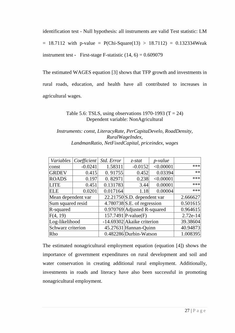
identification test - Null hypothesis: all instruments are valid Test statistic: LM
= 18.7112 with p-value = P(Chi-Square(13) > 18.7112) = 0.132334Weak
instrument test - First-stage F-statistic (14, 6) = 0.609079
The estimated WAGES equation [3] shows that TFP growth and investments in
rural roads, education, and health have all contributed to increases in
agricultural wages.
Table 5.6: TSLS, using observations 1970-1993 (T = 24) Dependent variable: NonAgricultural
Instruments: const, LiteracyRate, PerCapitaDevelo, RoadDensity,
RuralWageIndex, LandmanRatio, NetFixedCapital, priceindex, wages
Variables Coefficient Std. Error z-stat p-value const -0.0241 1.58311 -0.0152 <0.00001 *** GRDEV 0.415 0. 91755 0.452 0.03394 ** ROADS 0.197 0. 82971 0.238 <0.00001 *** LITE 0.451 0.131783 3.44 0.00001 *** ELE 0.0201 0.017164 1.18 0.00004 *** Mean dependent var 22.21750 S.D. dependent var 2.666627 Sum squared resid 4.780738 S.E. of regression 0.501615 R-squared 0.970769 Adjusted R-squared 0.964615 F(4, 19) 157.7491 P-value(F) 2.72e-14 Log-likelihood -14.69302 Akaike criterion 39.38604 Schwarz criterion 45.27631 Hannan-Quinn 40.94873 Rho 0.482286 Durbin-Watson 1.008395
The estimated nonagricultural employment equation (equation [4]) shows the
importance of government expenditures on rural development and soil and
water conservation in creating additional rural employment. Additionally,
investments in roads and literacy have also been successful in promoting
nonagricultural employment.
28 | P a g e
Table 5.7: TSLS, using observations 1970-1993 (T = 24) Dependent variable: PUIR
Instrumented: LandmanRatio, Yield
instruments: const, tfp, wages, r_d, per capita develo, production of food gross value output, gross vaa, net fixed capital, populationunder
Variables Coefficient Std. Error z-stat p-value Const -0.0302 19.27 -0.0016 <0.00001 *** IRE 0.118 0.146835 0.804 0.00219 *** ELE 0.032 0.3083.3 0.103 <0.00001 ***
Mean dependent var 4153.208 S.D. dependent var 998.2204 Sum squared resid 114043.5 S.E. of regression 77.47445 R-squared 0.995029 Adjusted R-squared 0.993982 F(4, 19) 5538.815 P-value(F) 7.65e-29 Rho -0.277046 Durbin-Watson 2.501505
Hausman test - Null hypothesis: OLS estimates are consistent, Asymptotic test
statistic: Chi-square (2) = 11.8847 with p-value = 0.00262583,Sargan over-
identification test - Null hypothesis: all instruments are valid Test statistic: LM
= 8.10671 with p-value = P (Chi-Square (5) > 8.10671) = 0.150452
Table 5.8: TSLS, using observations 1970-1993 (T = 24) Dependent variable: PRIP
instruments: const health wages villages electri road density per capita develo
populationunder
Variables Coefficient Std. Error z-stat p-value Const -0.00542 1.12399 -0.0048 <0.00001 *** PUIR 0.941 0.115564 8.147 0.01499 ** ELE 0.032 0.0681297 0.470 0.08197 *
Mean dependent var 29.33250 S.D. dependent var 3.947697 Sum squared resid 2.209573 S.E. of regression 0.350363 R-squared 0.993836 Adjusted R-squared 0.992123 F(5, 18) 580.3959 P-value(F) 3.14e-19 Log-likelihood -5.431468 Akaike criterion 22.86294 Schwarz criterion 29.93126 Hannan-Quinn 24.73816 Rho 0.043849 Durbin-Watson 1.677281
29 | P a g e
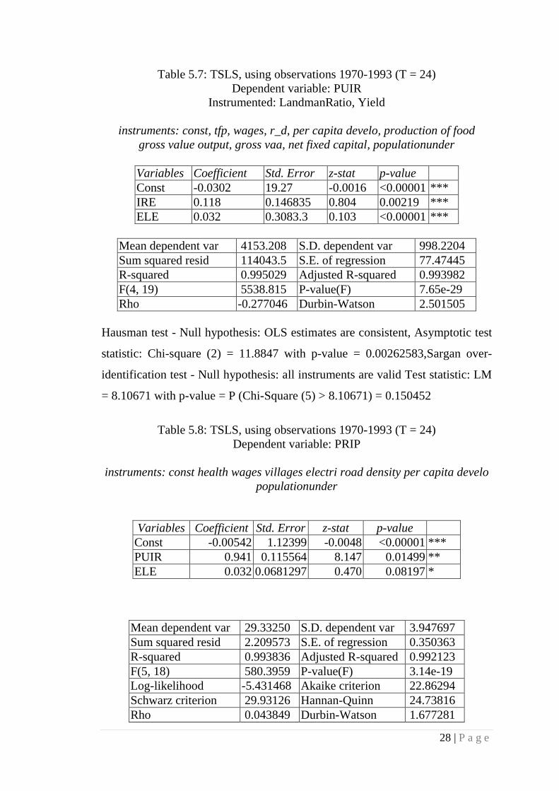
The estimated public irrigation equation (equation [5]) confirms that the
percentage of the cropped area under canal irrigation is primarily a result of
government investment, and that this has also been a significant catalytic force
in driving private investment in well and tube-well irrigation (equation [6]).
Improvements in the terms of trade seem not to have been a significant factor
in encouraging either public or private investment in irrigation.
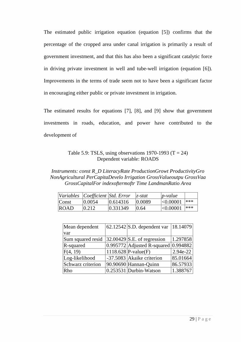
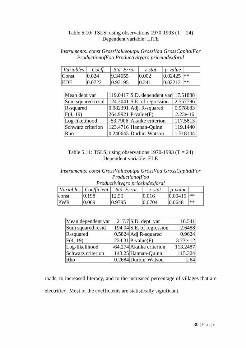
The estimated results for equations [7], [8], and [9] show that government
investments in roads, education, and power have contributed to the
development of
Table 5.9: TSLS, using observations 1970-1993 (T = 24) Dependent variable: ROADS
Instruments: const R_D LiteracyRate ProductionGrowt ProductivityGro NonAgricultural PerCapitaDevelo Irrigation GrossValueoutpu GrossVaa
GrossCapitalFor indexoftermoftr Time LandmanRatio Area
Variables Coefficient Std. Error z-stat p-value Const 0.0054 0.614316 0.0089 <0.00001 *** ROAD 0.212 0.331349 0.64 <0.00001 ***
Mean dependent var
62.12542 S.D. dependent var 18.14079
Sum squared resid 32.00429 S.E. of regression 1.297858 R-squared 0.995772 Adjusted R-squared 0.994882 F(4, 19) 1118.628 P-value(F) 2.94e-22 Log-likelihood -37.5083 Akaike criterion 85.01664 Schwarz criterion 90.90690 Hannan-Quinn 86.57933 Rho 0.253531 Durbin-Watson 1.388767
30 | P a g e
Table 5.10: TSLS, using observations 1970-1993 (T = 24) Dependent variable: LITE
Instruments: const GrossValueoutpu GrossVaa GrossCapitalFor
ProductionofFoo Productivitygro priceindexforal
Variables Coeff. Std. Error z-stat p-value Const 0.024 9.34655 0.002 0.02425 ** EDE 0.0722 0.93195 0.241 0.02212 **
Mean dept var 119.0417 S.D. dependent var 17.51888 Sum squared resid 124.3041 S.E. of regression 2.557796 R-squared 0.982391 Adj. R-squared 0.978683 F(4, 19) 264.9921 P-value(F) 2.23e-16 Log-likelihood -53.7906 Akaike criterion 117.5813 Schwarz criterion 123.4716 Hannan-Quinn 119.1440 Rho 0.240645 Durbin-Watson 1.518104
Table 5.11: TSLS, using observations 1970-1993 (T = 24) Dependent variable: ELE
Instruments: const GrossValueoutpu GrossVaa GrossCapitalFor
ProductionofFoo Productivitygro priceindexforal
Variables Coefficient Std. Error z-stat p-value const 0.198 12.55 0.016 0.00415 ** PWR 0.069 0.9795 0.0704 0.0648 **
Mean dependent var 217.7 S.D. dept. var 16.541 Sum squared resid 194.04 S.E. of regression 2.6488 R-squared 0.5824 Adj R-squared 0.9624 F(4, 19) 234.31 P-value(F) 3.73e-12 Log-likelihood -64.274 Akaike criterion 113.2487 Schwarz criterion 143.25 Hannan-Quinn 115.324 Rho 0.2684 Durbin-Watson 1.64
roads, to increased literacy, and to the increased percentage of villages that are
electrified. Most of the coefficients are statistically significant.
31 | P a g e
Table 5.12: TSLS, using observations 1970-1993 (T = 24) Dependent variable: LAND
Instruments: const GrossValueoutpu GrossVaa GrossCapitalFor ProductionofFoo
Productivitygro priceindexforal
Variables Coeff. Std. Error z-stat p-value Const 0.0257 16.54 0.00155 0.0658 ** TFP 0.0199 0.984 0.0202 0.0714 **
Mean depet var 121.847 S.D. dependent var 16.411 Sum squared resid 126.351 S.E. of regression 2.963 R-squared 0.9471 Adjusted R-squared 0.9526 F(4, 19) 233.541 P-value(F) 2.27e-19 Log-likelihood -62.318 Akaike criterion 116.291 Schwarz criterion 136.95 Hannan-Quinn 118.301 Rho 0.28142 Durbin-Watson 1.543
Table 5.13: TSLS, using observations 1970-1993 (T = 24)
Dependent variable: TT
Instruments: const GrossValueoutpu GrossVaa GrossCapitalFor ProductionofFoo
Productivitygro priceindexforal Variables Coefficient Std. Error z-stat p-value Const 0.0204 17.248 0.0012 0.0291 ** TFP -0.147 0.898 -0.164 0.0220 **
Mean dependent var 119.0417 S.D. dependent var 17.51888 Sum squared resid 124.3041 S.E. of regression 2.557796 R-squared 0.982391 Adjusted R-squared 0.978683 F(4, 19) 264.9921 P-value(F) 2.23e-16 Log-likelihood -53.79065 Akaike criterion 117.5813 Schwarz criterion 123.4716 Hannan-Quinn 119.1440 Rho 0.240645 Durbin-Watson 1.518104
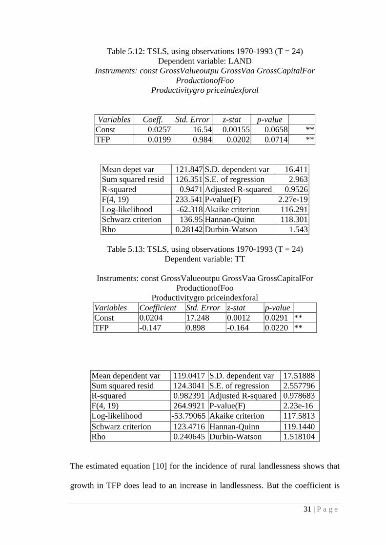
The estimated equation [10] for the incidence of rural landlessness shows that
growth in TFP does lead to an increase in landlessness. But the coefficient is
32 | P a g e
small and statistically insignificant. This may be due to the interpolation of
missing observations of the landless variable. Finally, the estimated terms of
trade equation (equation [11]) confirms that increases in TFP at the national
and state levels do exert a downward pressure on agricultural prices, worsening
the terms of trade for agriculture. It also shows that domestic agricultural prices
are highly correlated with world agricultural prices.
The estimated model shows clearly that improvements in agricultural
productivity not only reduce rural poverty directly by increasing income, but
they also reduce poverty indirectly by improving wages and lowering
agricultural prices. On the other hand, improvements in agricultural
productivity contribute to worsening poverty by increasing landlessness,
though this effect is relatively small.
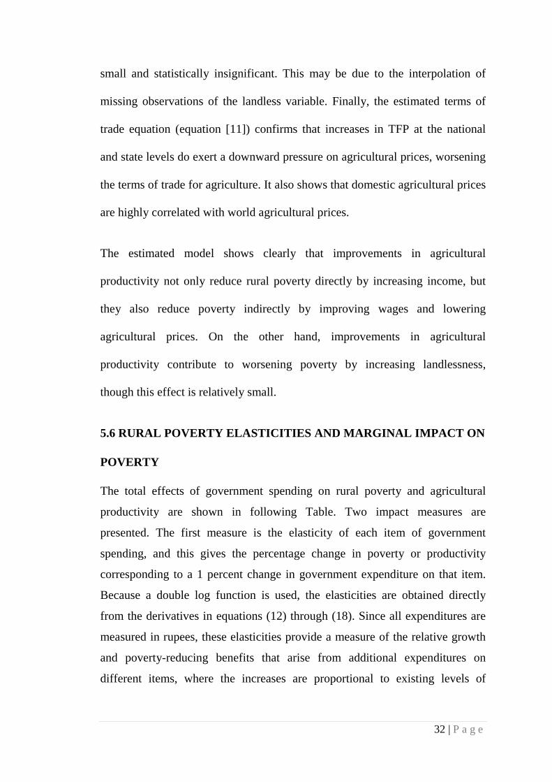
5.6 RURAL POVERTY ELASTICITIES AND MARGINAL IMPACT ON
POVERTY
The total effects of government spending on rural poverty and agricultural
productivity are shown in following Table. Two impact measures are
presented. The first measure is the elasticity of each item of government
spending, and this gives the percentage change in poverty or productivity
corresponding to a 1 percent change in government expenditure on that item.
Because a double log function is used, the elasticities are obtained directly
from the derivatives in equations (12) through (18). Since all expenditures are
measured in rupees, these elasticities provide a measure of the relative growth
and poverty-reducing benefits that arise from additional expenditures on
different items, where the increases are proportional to existing levels of
33 | P a g e
expenditure. The total elasticities for each expenditure item are decomposed
into their various direct and indirect components in Figures 1 to 7.
TABLE: 5.14 AFFECT ON POVERTY AND TFP OF ADDITIONAL GOVERNMENT EXPENDITURES
Expenditure Variables
Elasticities Marginal Impact of Spending Rs. 100 billion at 1993 prices
No. of poor reduced/ Rs. Million spent Poverty TFP Poverty TFP
R & D -0.0470* (1)
0.274* (1)
-0.442* (2)
5.65* (1)
89.1* (2)
Irrigation -0.0078 (5)
0.320* (4)
-0.034 (6)
0.54* (3)
6.5 (5)
Roads -0.0320* (3)
0.0715* (2)
-0.821* (1)
3.01* (2)
159.2* (1)
Education -0.0350* (2)
0.0422* (3)
-0.152* (3)
0.40* (4)
29.4* (3)
Power -0.0006 (6)
0.0007 (5)
-0.015 (7)
0.015 (5)
2.88 (7)
Rural Devp. -0.0157* (4)
0 (6)
-0.13* (5)
0 (6)
26.42* (4)
Health -0.00009 (7)
0 (7)
-0.015 (4)
0 (7)
4.3 (6)
Note: Numbers in parentheses are ranks. TFP is total factor productivity. * Significance at 5%
The second measure is the marginal return (measured in poverty and
productivity units) for an additional Rs 100 billion of government expenditure.
This measure is directly useful for comparing the relative benefits of equal
incremental increases in expenditures on different items, and it provides crucial
information for policymakers in setting future priorities for government
expenditure in order to further increase productivity and reduce rural poverty.
The marginal returns were calculated by multiplying the elasticities by the ratio
of the poverty or productivity variable to the relevant government expenditure
item in 1993. The Table also shows the number of poor people who would be
34 | P a g e
raised above the poverty line for each Rs 1 million of additional investment in
an expenditure item. An important feature of the results in effect on Table is
that all the productivity-enhancing investments considered offer a “win-win”
strategy for reducing poverty, while increasing agricultural productivity at the
same time. There appear to be no trade-offs between these two goals. However,
there are sizable differences in the productivity gains and poverty reductions
obtained for incremental increases in each expenditure item.
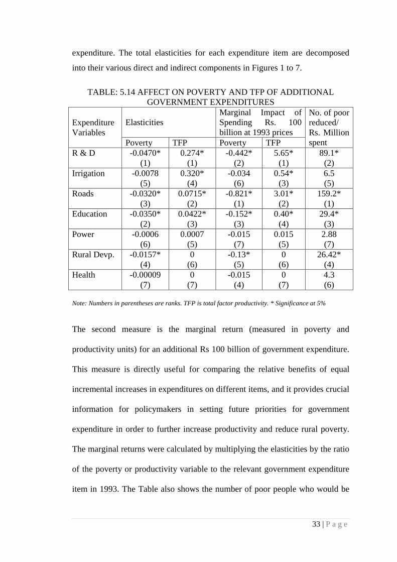
FIGURE: 5.3 EFFECTS ON POVERTY OF GOVERNMENTAL EXPENDITURES ONAGRICULTURAL RESEARCH AND
DEVELOPMENT
0.274
-0.147 0.104 0.0199
0.17 -0.152 -0.224 0.0002
Total Poverty Effects: �"
�#$% � &0.0470
Effect on poverty per billion rupees spent = -0.442
RED
TFP
PRICES
WAGES
LANDLESS
POVERTY
35 | P a g e
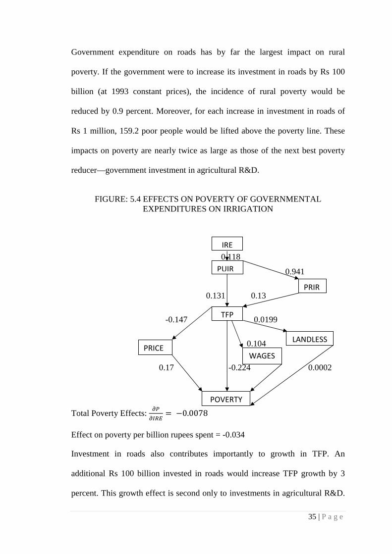
Government expenditure on roads has by far the largest impact on rural
poverty. If the government were to increase its investment in roads by Rs 100
billion (at 1993 constant prices), the incidence of rural poverty would be
reduced by 0.9 percent. Moreover, for each increase in investment in roads of
Rs 1 million, 159.2 poor people would be lifted above the poverty line. These
impacts on poverty are nearly twice as large as those of the next best poverty
reducer—government investment in agricultural R&D.
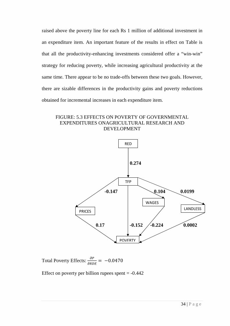
FIGURE: 5.4 EFFECTS ON POVERTY OF GOVERNMENTAL EXPENDITURES ON IRRIGATION
0.118
0.941
0.131 0.13
-0.147 0.0199
0.104
0.17 -0.224 0.0002
Total Poverty Effects: �"
�*#% � &0.0078
Effect on poverty per billion rupees spent = -0.034
Investment in roads also contributes importantly to growth in TFP. An
additional Rs 100 billion invested in roads would increase TFP growth by 3
percent. This growth effect is second only to investments in agricultural R&D.
IRE
PUIR
PRIR
TFP
PRICELANDLESS
WAGES
POVERTY
36 | P a g e
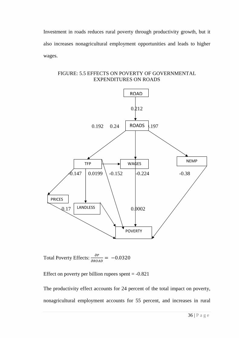
Investment in roads reduces rural poverty through productivity growth, but it
also increases nonagricultural employment opportunities and leads to higher
wages.
FIGURE: 5.5 EFFECTS ON POVERTY OF GOVERNMENTAL EXPENDITURES ON ROADS
0.212
0.212
0.192 0.24 0.197
-0.147 0.0199 -0.152 -0.224 -0.38
0.17 0.0002
Total Poverty Effects: �"
�#,-$ � &0.0320
Effect on poverty per billion rupees spent = -0.821
The productivity effect accounts for 24 percent of the total impact on poverty,
nonagricultural employment accounts for 55 percent, and increases in rural
ROAD
ROADS
TFP WAGES NEMP
PRICES
LANDLESS
POVERTY
37 | P a g e
wages account for the remaining 31 percent. Of the total productivity effect on
poverty, 75 percent arises from the direct impact of roads in increasing
incomes, while the remaining 25 percent arises from lower agricultural prices
(15 percent) and increased wages (10 percent). An increase in the incidence of
landlessness arising from the induced productivity growth has no significant
impact on rural poverty. Government investment in agricultural research and
development (R&D) has the second largest effect on rural poverty, but the
largest impact of any investment on growth in TFP. Another Rs 100 billion of
investment in R&D would increase TFP growth by almost 7 percent and reduce
the incidence of rural poverty by 0.5 percent. Moreover, another Rs 1 million
spent on R&D would raise 91 poor people above the poverty line. R&D has a
smaller impact on poverty than roads because it only affects poverty through
improved productivity, and it has not been particularly targeted to the poor by
the government. If future agricultural R&D was more deliberately targeted to
the poor, it might well have a greater impact on poverty (Hazell and Fan 1998).
Government spending on education has the third largest impact on rural
poverty reduction. An additional Rs 1 million spent on education would raise
32 poor people above the poverty line. Most of this effect arises from greater
nonfarm employment opportunities and increased wages. Education, at least
when measured as a simple literacy ratio, as it is here, has only a modest
impact on growth in agriculture’s TFP. Government expenditure on rural
development has the fourth largest impact on poverty reduction. Another Rs. 1
million of expenditure would raise 28 poor people above the poverty line, an
38 | P a g e
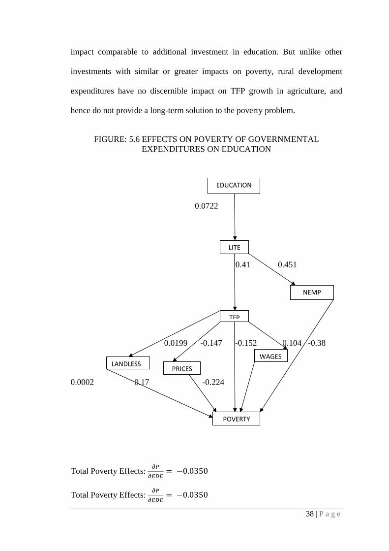
impact comparable to additional investment in education. But unlike other
investments with similar or greater impacts on poverty, rural development
expenditures have no discernible impact on TFP growth in agriculture, and
hence do not provide a long-term solution to the poverty problem.
FIGURE: 5.6 EFFECTS ON POVERTY OF GOVERNMENTAL EXPENDITURES ON EDUCATION
0.0722
0.41 0.451
0.0199 -0.147 -0.152 0.104 -0.38
0.0002 0.17 -0.224
Total Poverty Effects: �"
�%$% � &0.0350
Total Poverty Effects: �"
�%$% � &0.0350
EDUCATION
LITE
TFP
WAGES
NEMP
LANDLESS PRICES
POVERTY
39 | P a g e
Effect on poverty per billion rupees spent = -0.152
Government expenditure on irrigation has the fifth largest impact on rural
poverty reduction. Another Rs. 1 million of expenditure would raise 7 poor
people above the poverty line. However, public irrigation investments have the
third largest impact on TFP growth; an additional Rs 100 billion would add 0.6
percent to the TFP growth rate. Public irrigation affects poverty through its
impact on productivity, and this impact is enhanced by its catalytic role in
stimulating additional private investment in irrigation. Government expenditure
on power has positive but small and statistically insignificant impacts on both
rural poverty and productivity growth.
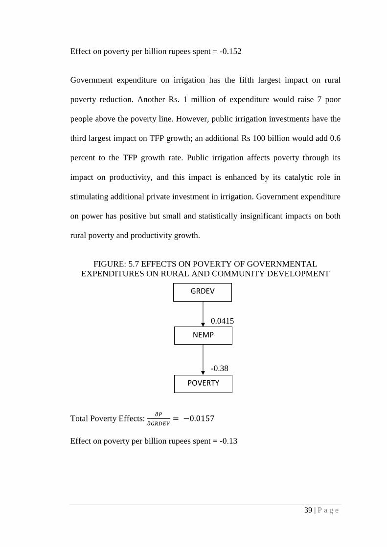
FIGURE: 5.7 EFFECTS ON POVERTY OF GOVERNMENTAL EXPENDITURES ON RURAL AND COMMUNITY DEVELOPMENT
0.0415
-0.38
Total Poverty Effects: �"
�/#$%0 � &0.0157
Effect on poverty per billion rupees spent = -0.13
GRDEV
NEMP
POVERTY
40 | P a g e
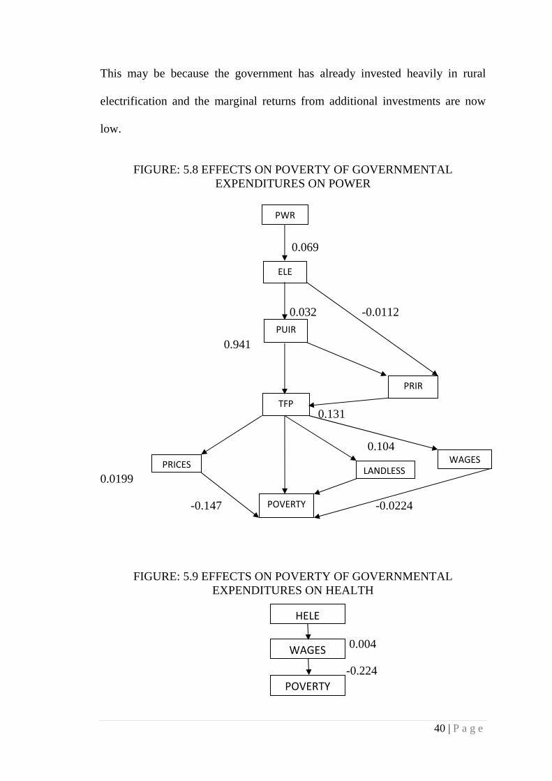
This may be because the government has already invested heavily in rural
electrification and the marginal returns from additional investments are now
low.
FIGURE: 5.8 EFFECTS ON POVERTY OF GOVERNMENTAL EXPENDITURES ON POWER
0.069
0.032 -0.0112
0.941
0.131
0.104
0.0199
-0.147 -0.0224
FIGURE: 5.9 EFFECTS ON POVERTY OF GOVERNMENTAL EXPENDITURES ON HEALTH
0.004
-0.224
HELE
WAGES
PWR
ELE
PUIR
TFP
POVERTY
PRIR
LANDLESS
WAGES PRICES
POVERTY
41 | P a g e
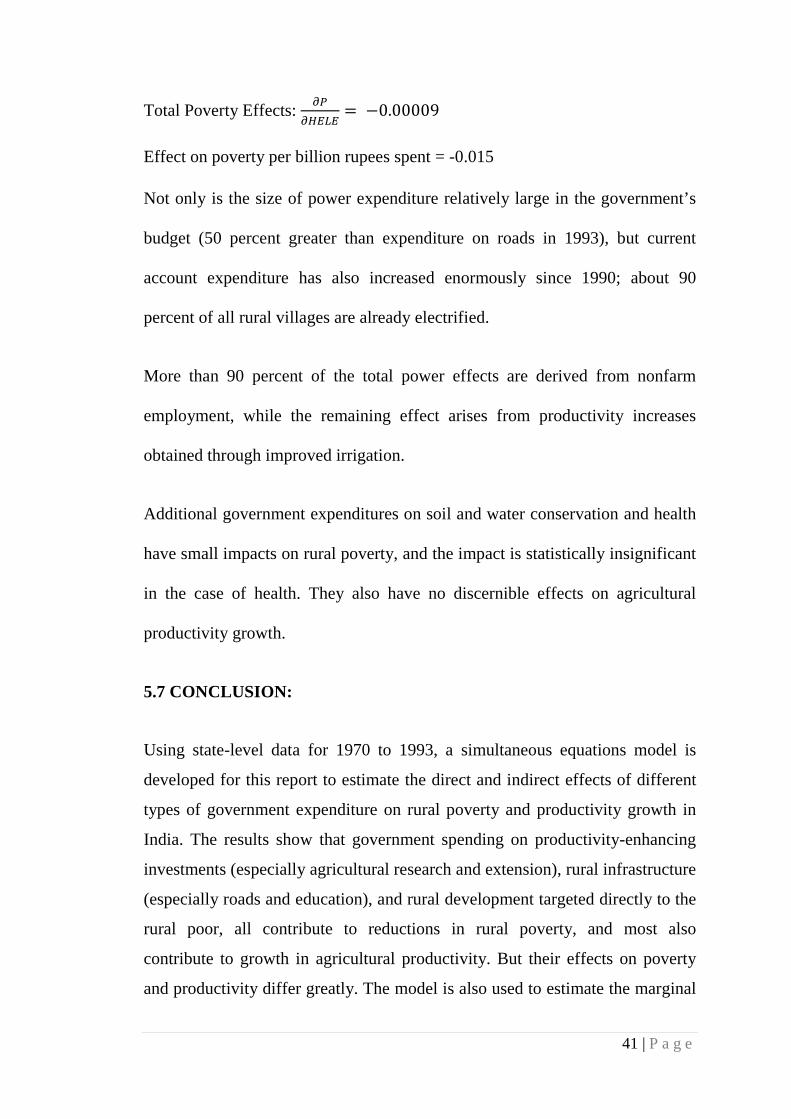
Total Poverty Effects: �"
�1%2% � &0.00009
Effect on poverty per billion rupees spent = -0.015
Not only is the size of power expenditure relatively large in the government’s
budget (50 percent greater than expenditure on roads in 1993), but current
account expenditure has also increased enormously since 1990; about 90
percent of all rural villages are already electrified.
More than 90 percent of the total power effects are derived from nonfarm
employment, while the remaining effect arises from productivity increases
obtained through improved irrigation.
Additional government expenditures on soil and water conservation and health
have small impacts on rural poverty, and the impact is statistically insignificant
in the case of health. They also have no discernible effects on agricultural
productivity growth.
5.7 CONCLUSION:
Using state-level data for 1970 to 1993, a simultaneous equations model is
developed for this report to estimate the direct and indirect effects of different
types of government expenditure on rural poverty and productivity growth in
India. The results show that government spending on productivity-enhancing
investments (especially agricultural research and extension), rural infrastructure
(especially roads and education), and rural development targeted directly to the
rural poor, all contribute to reductions in rural poverty, and most also
contribute to growth in agricultural productivity. But their effects on poverty
and productivity differ greatly. The model is also used to estimate the marginal
42 | P a g e
returns to agricultural productivity growth and poverty reduction obtainable
from additional government expenditures on different technology,
infrastructure, and social investments. Additional government expenditure on
roads is found to have the largest impact on poverty reduction as well as a
significant impact on productivity growth. It is a dominant “win-win” strategy.
Additional government spending on agricultural research and extension has the
largest impact on agricultural productivity growth, and it also leads to large
benefits for the rural poor. It is another dominant “win-win” strategy.
Additional government spending on education has the third largest impact on
rural poverty reduction, largely as a result of the increases in nonfarm
employment and rural wages that it induces. Additional irrigation investment
has the third largest impact on growth in agricultural productivity and a smaller
impact on rural poverty reduction, even allowing for trickle-down benefits.
Additional government spending on rural and community development,
including Integrated Rural Development Programs, contributes to reductions in
rural poverty, but its impact is smaller than expenditures on roads, agricultural
R&D, and education. Additional government expenditures on soil and water
conservation and health have no impact on productivity growth, and their
effects on poverty alleviation through employment generation and wage
increases are also small. The results of this study have important policy
implications. In order to reduce rural poverty, the Indian government should
give priority to increasing its spending on rural roads and agricultural research
and extension. These types of investment not only have a large impact on
poverty per rupee spent, but they also produce the greatest growth in
agricultural productivity. Additional government spending on irrigation has
substantial productivity effects, but no discernible impact on poverty reduction.
The impact of government spending on power is smaller than other
productivity-enhancing investments, and its poverty effect is also small. While
these investments have been essential in the past for sustaining agricultural
growth, the levels of investment stocks achieved may now be such that it may
be more important to maintain those current stocks rather than to increase them
43 | P a g e
further. Additional government spending on rural development is an effective
way of helping the poor in the short term, but since it has little impact on
agricultural productivity, it contributes little to long-term solutions to the
poverty problem.