Chapter 5: Statistics for Radiation Measurement · International Atomic Energy Agency ... Chapter 5: Statistics for ... 5.2.1.1. Data set as a list . Nuclear Medicine Physics:

IAEA International Atomic Energy Agency

Objective: To familiarize the student with the fundamental concepts of statistics for radiation measurement

Slide set prepared in 2015 by J. Schwartz (New York, NY, USA)

Slide set of 120 slides based on the chapter authored by M.G. LÖTTER of the IAEA publication (ISBN 978–92–0–143810–2): Nuclear Medicine Physics: A Handbook for Teachers and Students

Chapter 5: Statistics for Radiation Measurement

IAEA

CHAPTER 5 TABLE OF CONTENTS

5.1. Sources of error in nuclear medicine measurement 5.2. Characterization of data 5.3. Statistical models 5.4. Estimation of the precision of a single measurement in sample counting and imaging 5.5. Propagation of error 5.6. Applications of statistical analysis 5.7. Application of statistical analysis: detector performance

Nuclear Medicine Physics: A Handbook for Teachers and Students – Chapter 5 – Slide 2/120

IAEA

5.1. SOURCES OF ERROR IN NUCLEAR MEDICINE MEASUREMENT

Types of measurement errors:

• Blunders

• Systematic errors or accuracy of measurements

• Random errors or precision of measurements


IAEA


Blunders • Produce grossly inaccurate results

• Easily detected by experienced observers

• Radiation counting examples • Incorrect energy window setting

• Counting heavily contaminated samples

• Using contaminated detectors

• High activities leading to excessive dead time effects

• Selecting wrong patient orientation during imaging


IAEA

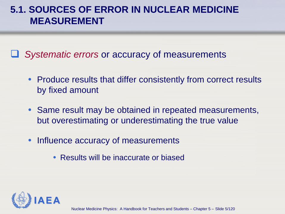
Systematic errors or accuracy of measurements

• Produce results that differ consistently from correct results by fixed amount

• Same result may be obtained in repeated measurements, but overestimating or underestimating the true value

• Influence accuracy of measurements

• Results will be inaccurate or biased



IAEA


• Not always easy to detect measurements may not be too different from expected results

• Can be detected using reference standards

• For example, use calibrated radionuclide reference standards to calibrate source calibrators to determine correction factors for each radionuclide used for patient treatment and diagnosis



IAEA


• Results can differ from true value by • constant value • and/or by a fraction

• Calculate regression curve using ‘golden standard’ reference values

• Use regression curve to convert systematic errors to more accurate value

• Example: Correlate ejection fraction determined by radionuclide gated study with the ‘golden standard’ values



IAEA

Systematic errors or accuracy of measurements • Examples:

• Dose measured with incorrectly calibrated ionization chamber

• Dead time losses when 123I reference standard measured • Thyroid uptake percentage will be overestimated

• Counting geometry different when counting samples vs reference sample



IAEA


• Examples:

• Tracer leaks out of blood compartment in blood volume measurements

• Will consistently overestimate the measured blood volume

• Selected background counts underestimate true ventricular background during gated blood pool studies

• Ejection fraction will be consistently underestimated



IAEA

Random errors or precision of measurements

• Variations in results from one measurement to next

• Arise from: • Actual random variation of measured quantity • Physical limitations of measurement system

• Affect measurement: • Reproducibility • Precision • Uncertainty



IAEA

Random errors always present in radiation measurements

• Radionuclide decay is a randomly varying quantity • 57Co energy spectrum • Source in scattering medium • Measured with scintillation detector • Variation around solid line is due to random error introduced

by radionuclide decay



IAEA


Random errors also play a significant role in radionuclide imaging

• Radionuclide decay errors significantly influence image visual quality

• Number of counts (N) in each pixel is subject to random error • Relative random error decreases as counts per pixel

increases


IAEA


As Ntotal increases

• Nper pixel increases • Random error decreases • Results in improved visual image quality • Increases ability to visualize:

• Anatomical structures • Tumor volumes


IAEA


Measuring system/imaging device random error influences image quality

• Results from energy resolution & intrinsic spatial resolution • Influenced by random errors during the detection of each

gamma photon • Determines ability to reject lower energy scattered gamma

photons and improve image contrast


IAEA


The visual effect of the random error as a result of the measured quantity

• 99mTc-planar bone scans (acquired on a 256×256 matrix) were acquired with a scintillation camera

• Acquisition was terminated at 21, 87 and 748 kcnts


IAEA


Measurement may be precise (small random error) but inaccurate (large systematic error), or vice versa

Example: Calculation of the ejection fraction during gated cardiac studies • Background region of interest (ROI) selection will be exactly

reproducible using software algorithm

• Algorithm may select ROI that does not reflect true ventricular background

• Measurement will be precise but inaccurate


IAEA


Individual radiation counts of a radioactive sample may be imprecise due to random error, but average value of a number of measurements will be accurate

It’s important to analyse the random errors to determine the associated uncertainty

• Done using methods of statistical analysis


IAEA

Measures of central tendency of data set: • Mean (average) • Median

Measures of variability, random error and precision of data set: • Variance • Standard deviation • Fractional standard deviation

Examples: • Data set obtained from long lived radioactive sample

5.2. CHARACTERIZATION OF DATA 5.2.1. Measures of central tendency and variability 5.2.1.1. Data set as a list


IAEA

Examples:

• Data set obtained from long lived radioactive sample

• Counted repeatedly • All done under same conditions • Properly operating counting system

• Sample disintegration rate has random variations from one moment to next

• Number of counts recorded in successive measurements is not the same

• Due to random errors



IAEA

Calculation for experimental mean of a data set:

• N independent measurements of same physical quantity • x1, x2, x3, ….xi……xN

• The mean given by:

1 2e

1

N

N

ii

x x xxN

x

N=

+ + +=

=∑



IAEA

Procedure for obtaining median

• Sort list of measurements by size • Median:

• Middlemost measurement if N is odd • Average of 2 middlemost measurements if N is even • Example

• N=5 • Measurements: 7, 13, 6, 10 and 14 • Sorted by size: 6, 7, 10, 13 and 14 • Median = 10

• Less affected by outliers than the mean • Outlier is a blunder

• Much greater or much less than the others.



IAEA

Variance:

Standard Deviation:

Fractional standard deviation, σeF (fractional error or coefficient of variation) :

• Inverse of σeF referred to as the signal to noise ratio.

2e eσ σ=

eeF

exσσ =



IAEA

Often convenient to represent data set by relative frequency distribution function F(x)

• F(x) = measured value relative frequency

• F(x) is normalized:

• Represents all information in original data set in list format

• Useful quick visual summary of measurement values distribution

• Can be used to identify outliers

5.2. CHARACTERIZATION OF DATA 5.2.1. Measures of central tendency and variability 5.2.1.2. Data set as a relative frequency distribution function

1)(0

=∑∞

=xxF

Number of occurrences of the value x in each bin( )F xN

=


IAEA

Example of relative frequency distribution application

• Scintillation counter measurements appear noisy due to random error

• Measurements fluctuate randomly around mean = 90 counts.



IAEA

• Plot shows relative frequency of measured counts

• X-axis = range of possible counts

• At 6 count intervals

• Y-axis = relative frequencies of particular count values occur

• Most common value = mean

• e.g. 26% of measurements in plot are near the mean = 90 counts

• Blue curve: expected calculated normal distribution

Histogram (red bars) of F(x) of measurements fluctuations



IAEA

Measures of central tendency using F(x):

• Mean (average)

• Median • Value at which integral of F(x) is 0.5 • Half of measurements will be < and half will be > median

• Mode

• Most frequent value OR • Value at maximum probability of F(x)



IAEA

Mean of F(x):

Experimental sample variance using F(x):



IAEA

F(x) provides insight on the precision of the experimental sample mean and of a single measurement

The value of the true mean is not usually known but the experimental sample mean can be used as an estimate of the true mean

( ) ( )t ex x≈



IAEA

Often impractical to obtain multiple measurements, especially for radionuclide imaging & nuclear measurements on patients

F(x) will determine precision of single measurement as an estimate of true value

Probability that single measurement will be close to t depends on the dispersion (relative width) F(x). This is expressed by the σ 2 or σ

The standard deviation σ is a number such that 68.3% of the measurement results fall within ±σ of t • I.e. If x= result of a given measurement, there is a 68.3% chance that is

within the range x ± σ • Called the 68.3% confidence interval for t



IAEA

CONFIDENCE LEVELS IN RADIATION MEASUREMENTS



IAEA

5.3. STATISTICAL MODELS

F(x) of many repetitions can be predicted under certain conditions

A measurement is defined as counting the number of successes x resulting from a given number of trials n.

Assumptions: • Only two results are possible for each trial (i.e. binary process): either a

success or not • Probability of success p is constant for all trials. • e.g.


IAEA

5.3. STATISTICAL MODELS

The third example gives the basis for counting nuclear radiation events

A trial consists of observing a given radioactive nucleus for a period of time t

The number of trials n = number of nuclei in the measured sample

Measurement consists of counting nuclei that undergo decay The probability of success, p, for radioactive decay:

• λ = radionuclide decay constant

(1 e )tp λ−= −


IAEA

5.3. STATISTICAL MODELS 5.3.1. When binomial, Poisson & normal distributions are applicable 5.3.1.1. Binomial distribution

This is the most general model and is widely applicable to all constant p processes.

Rarely used in nuclear decay applications.

Must be used is when a radionuclide with a very short half-life is counted with a high counting efficiency.


IAEA

5.3. STATISTICAL MODELS 5.3.1. When binomial, Poisson & normal distributions are applicable 5.3.1.2. Poisson distribution

Poisson distribution

• Direct mathematical simplification when probability of success p is small

• Must be used because experimental distribution is asymmetric but normal distribution is always symmetrical

For nuclear counting, used when:

• Observation time << T1/2 of source • Detection efficiency is low


IAEA

5.3. STATISTICAL MODELS 5.3.1. When binomial, Poisson & normal distributions are applicable 5.3.1.3. Gaussian or normal distribution

Gaussian (normal) distribution

• Further simplification of binomial if the mean number of successes is relatively large (>30)

• Experimental distribution will be symmetrical

All 3 model distributions becomes identical when: • p is small • Large enough number of trials such that the expected mean number of successes is large.


IAEA

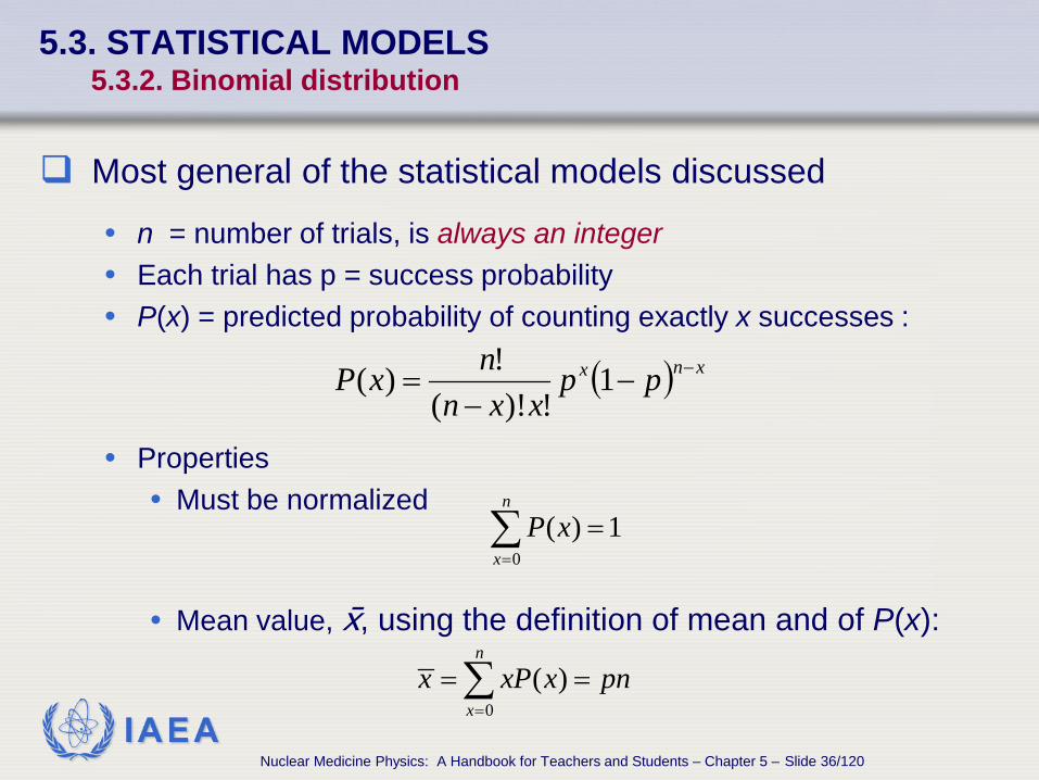
5.3. STATISTICAL MODELS 5.3.2. Binomial distribution

Most general of the statistical models discussed

• n = number of trials, is always an integer • Each trial has p = success probability • P(x) = predicted probability of counting exactly x successes :

• Properties

• Must be normalized

• Mean value, , using the definition of mean and of P(x):

( ) xnx ppxxn

nxP −−−

= 1!)!(

!)(

1)(0

=∑=

n

xxP

0( )

n

xx xP x pn

=

= =∑


IAEA


The predicted variance σ2 is given by:

• Substituting for P(x) and np, :

The standard deviation is:

( )22

0( )

xx x P xσ

∞

=

= −∑

( ) ( )2 1 1np p x pσ = − = −

( ) ( )1 1np p x pσ = − = −


IAEA


The fractional standard deviation σF is given by:

σ predicts amount of fluctuation inherent in binomial distribution in terms of n & p


IAEA

5.3. STATISTICAL MODELS 5.3.2. Binomial distribution 5.3.2.1. Application example of binomial distribution

The operation of a scintillation detector consists of:

• Scintillation crystal mounted on photomultiplier (PMT) in a light tight construction

• Photon interacts with crystal & generates n light γ ’s

• Light γ ’s eject x electrons (e-) from PMT photocathode

• Electrons multiplied to form pulse that can be further processed

• n, x & multiplication factor vary statistically during γ detection

• This variation determines the energy resolution of the system


IAEA


Example: ejection of e-'s from photocathode

• Typical scintillation counter values for 142 keV 99mTc γ ’s:

• Need: 100eV per scintillation γ

• n = 142 000 eV/100eV/photon = 1420 light photons emitted

• x electrons generate these fall on PMT photocathode per gamma ray absorbed.

• 5 light γ ’s required to eject one e-

• Binomial distribution probability of light γ ejecting an e- is:

p = 1/5


IAEA

• Predicted mean number of e-'s ejected per gamma ray:

• σ & σF for x (no. of e-'s ejected) calculated using binomial distribution:


-e 248142051

=×== pnx

( ) 11 284 1 155

x pσ = − = − =

( ) ( )F

1 1 1/ 5 0.053

284p

xσ

− −= = =


IAEA


• The electron ejection stage at the photocathode contributes 5.3% to the overall σ

• The variation in x will influence the pulse height obtained for each gamma ray.

• The variation in the pulse height during the detection of gamma rays will determine the width of the photopeak and the energy resolution of the system


IAEA

5.3. STATISTICAL MODELS 5.3.3. Poisson distribution

Examples of binary processes characterized by low probability of success for each individual trial:

• Nuclear counting & imaging applications with • large numbers of radionuclides in sample • Nuclear counting & imaging applications with large number of trials • Relatively small fraction gives rise to recorded counts.

• Administered imaging radionuclide: • For every gamma that interacts with tissue many are emitted • Many gammas strike the detector for every single recorded interaction.

• Approximation of small p holds under these conditions • Some mathematical simplifications can be applied to the

binomial distribution.


IAEA


Poisson distribution • The binomial distribution reduces to the form:

• pn= holds for this distribution

• Final form: • Only one parameter to get P(x):

• Useful when: • can be measured/estimated • there is no information about p or n • e.g. nuclear counting and imaging

( )!e)(

xpnxP

pnx −

=

( )!e)(

xxxP

xx −

=


IAEA


Poisson distribution properties • Normalized frequency distribution • Mean value (or first moment) same as that of the binomial

distribution:

• Predicted variance differs from that of the binomial distribution :

• Predicted standard deviation & fractional standard deviation σF :

pnxxPxx

== ∑∞

=0)(

( ) xpnxPxxx

==−= ∑∞

=0

22 )(σ

x== 2σσσ

σσ 11F ===

xx


IAEA

5.3. STATISTICAL MODELS 5.3.4. Normal distribution

Normal distribution • p<1 & > 30 • The binomial distribution reduces to the form:

• Only defined for integer values of x • Always symmetrical or ‘bell-shaped’ • Properties shared with the Poisson distribution:

• It is normalized • Characterized by a single parameter • Predicted variance: σ 2 = • Predicted standard : σ =√ • Predicted fractional standard deviation: σF=1/σ

2( )21( ) e

2

x xxP x

πx

−−

=


IAEA

5.3. STATISTICAL MODELS 5.3.4. Normal distribution 5.3.4.1. Continuous normal distribution: confidence intervals

Number of possible sample outcomes increases with sample size

As the sample size approaches infinity the distribution becomes continuous

Some random variables are essentially continuous and have continuous distributions (e.g. such as height and weight)

In these situations, p is not small as was assumed for the discrete Poisson and normal distributions, and the equation does not apply

The continuous normal distribution is given by:

2

21

e2

1)(

−

−= σ

πσ

xx

xP


IAEA


Continuous normal distribution properties:

• Continuous • Symmetrical • Both tails extend to infinity • Mean = median = mode • Described by 2 parameters:

• mean • Determines location curve centre

• standard deviation σ • Represents the spread around


IAEA


Of the total curve area:

• 68% between ± σ • 95% between ± 2σ • 99.7% between ± 3σ


IAEA

5.3. STATISTICAL MODELS 5.3.4. Normal distribution 5.3.4.2. Continuous normal distribution: applications in medical physics

Normal distribution often used to fit experimental data

The equation is modified so that the maximum value of the distribution at is normalized to 100:

212( ) 100 e

x x

P x σ− −

=


IAEA

The spatial resolution of imaging devices t is determined as the full width at half maximum (FWHM) of a normal distribution fitted to point or line spread function

Relationship between FWHM & σ for a normal distribution: • setting P(x) = 50 and solving

σ355.2FWHM =



IAEA

Example:

Line source response for a scintillation camera Fitted to a normal distribution σ = 10mm Image resolution = FWHM = 23.6 mm



IAEA

The photopeak in nuclear spectroscopy can be fitted to a normal distribution

Fractional energy resolution, RE , of scintillation detectors:

The energy spectrum in medical physics applications is measured in kiloelectronvolts (keV) or megaelectronvolts (MeV)

EFWHM 2.355R

E Eσ

= =



IAEA

5.4. ESTIMATION OF THE PRECISION OF A SINGLE MEASUREMENT IN SAMPLE COUNTING AND IMAGING 5.4.1. Assumption

Counting statistics is useful when a single measurement of a quantity is available & the uncertainty associated with that measurement is required

The square root of the sample variance, σ • Measure of deviation of any one measurement from the

true mean • Serves as an index of degree of precision associated with

a measurement from that set


IAEA


For a single measurement, x, is available

• Sample variance cannot be calculated directly

• σ must be estimated by analogy with appropriate statistical model

• Appropriate theoretical distribution matched to data if x is drawn from a population whose distribution is predicted by Poisson or Gaussian

• Assume the distribution mean = x

xx ≈


IAEA


Assuming x, P(x) is defined for all values of x

Expected sample variance, s2, expressed in terms of σ :

The best estimate of σ from , which should typify a single measurement x, is given by:

Assuming P(x) is Gaussian with large x

The range of values x ± σ (or x ±√x) will contain the true mean with a 68% probability

2s xσ= ≈

xxs ≈== 22 σ


IAEA


If x=100, then σ √x = √100 = 10

Conventional choice for quoting uncertainty of single measurement x: • x ± σ • Interval is expected to contain true mean with probability of

68% • Probability can be increased by expanding interval • Example:

• for P(x)=99%, interval must be expanded by 2.58σ • In the example, the range is 100 ± 25.8

The associated probability level should be stated under methods when errors are reported


IAEA


Options available in quoting uncertainty to be associated with a single measurement are shown


IAEA

5.4. ESTIMATION OF THE PRECISION OF A SINGLE MEASUREMENT 5.4.2. The importance of the fractional σF

The precision, σ, will increase proportionally to √x • i.e. if x increases, σ will also increase • Increase σ < increase in x

The relation σ & x is best demonstrated by calculating σF:

• The number of counts or single measurement value x completely determines σF

• σF decreases as x increases • Minimum number of counts must be accumulated to achieve

a given σF

xxx

x1

F ===σσ


IAEA

Example :

• If 100 counts recorded σF = 10%

• If 10 000 counts recorded σF = 1%

• Demonstrates the importance of acquiring enough counts to meet the required precision



IAEA

Easier to achieve σF when measuring samples in counting tubes than in vivo on patients

Single measurement from high activity sample will be obtained in a short time

To achieve same σF using low activity sample measurement time will have to be increased

Can be obtained by using automatic counters set to stop counting after a preset time or preset counts have been reached



IAEA

Single measurement precision is very important during imaging • Low precision obtained if number of counts (N) acquired in a

picture element or pixel is low

• There will then be a wide range of fluctuations between adjacent pixels

Poor image quality

Only possible to identify: large defect volumes or defects with a high contrast



IAEA

Detection of a defect requires that N from defect lie outside the background range: xb ± 2σb

N in a target volume will be determined by acquisition time, activity in target volume and the sensitivity of the measuring equipment



IAEA

Imaging equipment sensitivity can be increased by increasing spatial resolution in terms of FWHM

To obtain images with the max diagnostic value during visual interpretation there is a trade off between:

• Single sample counting precision

• Spatial resolution of imaging device



IAEA

Counting statistics are very important during image quantification

• Accumulated counts within a target volume (e.g. an organ) have to be accurately determined

• Accurate quantification requires corrections be made for: • Background activity • Attenuation • Scatter contributions • These procedures further reduce the precision of

quantification



IAEA

5.4. ESTIMATION OF THE PRECISION OF A SINGLE MEASUREMENT 5.4.3. Caution on the use of the estimate of the precision of a single measurement in sample counting and imaging

All conclusions based on measured number of success

Nuclear measurements/imaging • Single measurement precision using σ = √x can only be applied if x

represents number of events recorded in a given observation time • For example does not apply to: Counting rates Sums or differences of counts Averages of independent counts Pixel counts following tomographic image reconstruction Any derived quantity

Quantity calculated as function of number of recorded counts

Error must be calculated according to error propagation methods outlined


IAEA

• thyroid iodine uptake • ejection fraction • renal clearance

• blood volume • red cell survival time

5.5. PROPAGATION OF ERROR

Preceding section described methods for estimating random error or precision of single measurement

Most diagnostic nuclear medicine procedures involve multiple measurements/imaging procedures for calculation of results

• Examples:

Internal dosimetry is performed using nuclear

measurements and imaging data


IAEA


Corresponding precision in derived quantity is estimated by propagating initial measurement errors through the calculations performed to arrive at the result

The variables used in the calculation of errors must be independent to avoid correlation effects

Assumption: • Nuclear measurement error arises only from random

fluctuations in decay rate • Statistically independent of other errors


IAEA


Error propagation formulas apply to measurements obtained from

• Continuous distribution • Represented by x1, x2, x3... with variances σ(x1)2, σ(x2)2, σ(x3)2... • e.g. to estimate precision in height and weight measurements

• Poisson distributions • Represented by N1, N2, N3... with variances σ(N1)2, σ(N2)2,

σ(N3)2...

• Discrete normal distributions. • Represented by N1, N2, N3... with variances σ(N1)2, σ(N2)2,

σ(N3)2...


IAEA

If xs = x1 ± x2 ± x3 … • Variance :

• Standard deviation :

• Fractional standard deviation:

( ) ( ) ( ) ( ) 2

32

22

1321 xxxxxx σσσσ ++=±±

( ) ( ) ( ) ( ) 2

32

22

12

321 xxxxxx σσσσ ++=±±

( ) ( ) ( ) ( )2 2 21 2 3

F 1 2 31 2 3

x x xx x x

x x xσ σ σ

σ+ +

± ± =± ±

5.5. PROPAGATION OF ERROR 5.5.1. Sums and differences


IAEA

For measurements with Poisson or discrete normal distribution: • Variance :

• Standard deviation:


• Equations apply to mixed combinations of sums and differences

( ) 321321 NNNNNN ++=±±σ

( ) 3212

321 NNNNNN ±±=±±σ

( ) 1 2 3F 1 2 3

1 2 3

N N NN N N

N N Nσ

± ±± ± =

± ±



IAEA

The influence on σ & σF of adding/subtracting:



IAEA

Conclusions:

• σ is the same for N1 – N2 & N1 + N2 for the same values of N1 & N2

• σF for differences is large when the differences between the values are small

Background must be limited to as low a value as possible

• Imaging scatter/background corrections involve subtraction The statistical information deteriorates as a result of the increased uncertainty in the pixel values



IAEA

5.5. PROPAGATION OF ERROR 5.5.2. Multiplication and division by a constant

Multiplication: • xM = Ax, where A is a constant

Counting measurements / Poisson / discrete normal distribution: • xM = AN

xAσσ =M

xAxA xx σσσ ==F

NA=MσN1

F =σ


IAEA

5.5. PROPAGATION OF ERROR 5.5.2. Multiplication and division by a constant

Division:

• xD = x/B, where B is a constant.

Counting measurements / Poisson / discrete normal distribution:

• xD = N/B

Bxσσ =M xx

BB

xx σσσ ==F

BN

=Mσ N1

F =σ


IAEA

5.5. PROPAGATION OF ERROR 5.5.3. Products and ratios

The uncertainty in the product or ratio of a series of measurements x1, x2, x3... is expressed in terms of the fractional uncertainties in the individual results, σF(x1), σF(x2), σF(x3)...

• xP of measurements with continuous normal distribution:

• Fractional variance

• Fractional standard deviation

• Standard deviation

P 1 2 3 P 1 2 3 x x x x x x x x= × × = ÷ ÷

( ) ( ) ( ) ( ) 23F

22F

21F

2PF xxxx σσσσ ++=

( ) ( ) ( ) ( ) 23F

22F

21FPF xxxx σσσσ ++=

( ) ( ) ( ) ( )2 2 2P F 1 F 2 F 3 Px x x x xσ σ σ σ= + + ×


IAEA

5.5. PROPAGATION OF ERROR 5.5.3. Products and ratios

For counting / Poisson / discrete normal distribution measurements:

• xP of measurements with continuous normal distribution:

• Fractional variance

• Fractional standard deviation

• Standard deviation

P 1 2 3

P 1 2 3

N N N NN N N N

= × ×= ÷ ÷

( ) 321

2PF

111NNN

N ++=σ

( ) 321

PF111

NNNN ++=σ

( )P P1 2 3

1 1 1N NN N N

σ = + + ×


IAEA

5.6. APPLICATIONS OF STATISTICAL ANALYSIS 5.6.1. Multiple independent counts 5.6.1.1. Sum of multiple independent counts

If there are • n repeated counts from the same source • for equal counting times • the results of the measurements are N1, N2, N3....... Nn and their

sum is Ns, then:

σ for the sum of all counts is the same as if the measurement had been carried out by performing a single count, extending over the period represented by all of the counts.

s321sNNNNN =++= σ

321s NNNN ++=


IAEA

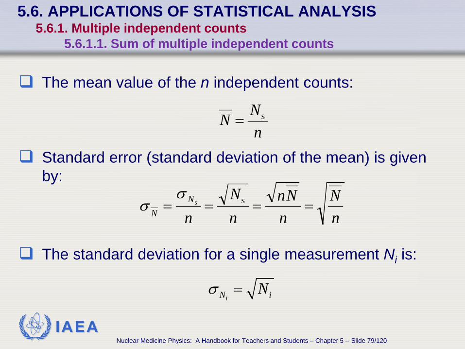
The mean value of the n independent counts:

Standard error (standard deviation of the mean) is given by:

The standard deviation for a single measurement Ni is:

nN

nNn

nN

nN

N ==== ssσ

σ

nNN s=

iN iNσ =

5.6. APPLICATIONS OF STATISTICAL ANALYSIS 5.6.1. Multiple independent counts 5.6.1.1. Sum of multiple independent counts


IAEA

5.6. APPLICATIONS OF STATISTICAL ANALYSIS 5.6.1. Multiple independent counts 5.6.1.2. Mean value of multiple independent counts

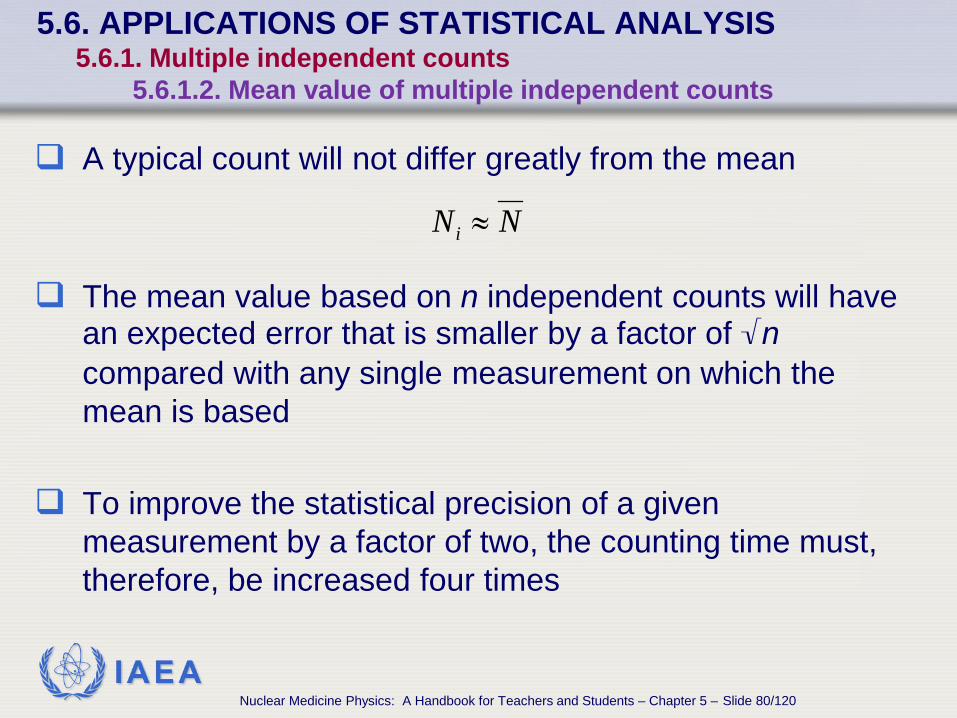
A typical count will not differ greatly from the mean

The mean value based on n independent counts will have

an expected error that is smaller by a factor of √n compared with any single measurement on which the mean is based

To improve the statistical precision of a given measurement by a factor of two, the counting time must, therefore, be increased four times

NNi ≈


IAEA

5.6. APPLICATIONS OF STATISTICAL ANALYSIS 5.6.2. Standard deviation & relative standard deviation for counting rates

If N counts are accumulated over time t, then the counting rate R is given by: • Assuming the time t is measured with a very small uncertainty, so

that t can be considered a constant

Uncertainty of counting rate (an application of the propagation of errors multiplying by a constant) :

Fractional standard deviation

tNR =

tR

tN

tx

R ===σσ

tRtRN

tRx 1

F ===σσ


IAEA

Sample 2: • R = 10 000 cps • Standard deviation:


5.6. APPLICATIONS OF STATISTICAL ANALYSIS 5.6.2. Standard deviation & relative standard deviation for R 5.6.2.1. Example: comparison of error of R & counts accumulated

Sample 1: • The counts acquired: N = 10 000 counts • Standard deviation: σN = 100 counts • Fractional standard deviation: σF = 0.01 = 1%

cps10100

10000==Rσ

%1.0001.010010000

1F ==

×=σ

The activity of two samples is measured

The counts acquired for samples 1 & 2 were numerically the same The uncertainties were very different Need to determine if value used is a single value or a value that has

been obtained by calculation


IAEA

5.6. APPLICATIONS OF STATISTICAL ANALYSIS 5.6.3. Effects of background counts

Background counts • Do not originate from the sample or target volume • Unwanted counts such as scatter

Background counts during sample counting consist of • Electronic noise • Detection of cosmic rays • Natural radioactivity in the detector • Down scatter radioactivity from non-target radionuclides in the

sample

Radiation from non-target tissue will also contribute to background during in vivo measurements • e.g. measurement of thyroid iodine uptake or left ventricular ejection

fraction


IAEA


Scattered radiation from target as well as non-target tissue will influence quantification and will be included in the background

If the background count is Nb, and the gross counts of the sample and background is Ng, then the net sample count Ns is:

Standard deviation for Ns

Fractional standard deviation for Ns

( )bg

bgsF NN

NNN

−

+=σ

bgs NNN −=

( ) bgs NNN +=σ


IAEA


If the background count rate is Rb, acquired in time tb, and the gross count rate of the sample and background is Rg, acquired in time tg, then the net sample counts Rs is:

Standard deviation for Rs

Fractional standard deviation for Ns

( )b

b

g

gs t

RtR

R +=σ

bgs RRR −=

( )

g b

g bF s

g b

R Rt t

RR R

σ+

=−


IAEA


If the same counting time t is used for both sample and background measurement:

• Standard deviation for Rs

• Fractional standard deviation for Ns

( )t

RRR bg

s

+=σ

( ) ( )g b

F sg b

R RR

t R Rσ

+=

−


IAEA

5.6. APPLICATIONS OF STATISTICAL ANALYSIS 5.6.3. Effects of background counts 5.6.3.1. Example: error in net target counts following background correction

Example: • Planar image of the liver is acquired for the detection

of tumours • ROI1 and ROI2 selected

• equal sized regions • cover 2 potential tumours

• Nb selected over normal tissue of the same area as ROI1 & ROI2

• ROI1 • Ng = 484 counts • Nb = 441counts

• ROI2 • Ng = 484 counts • Nb = 169 counts


IAEA


Example:

• Difference

• Error associated with the difference when Ng Nb :

( ) 7073.0441484441484

sF =−+

=Nσ

counts 43 441– 484 bgs ==−= NNN

( ) counts 4.30441484s =+=Nσ

( ) %7.70sP =Nσ


IAEA


Example:


IAEA


Conclusion:

σF and percentage σP significantly increase when the background increases relative to the net counts

It is important to acquire as many counts as possible to

decrease the uncertainty in detection of target volume radioactivity


IAEA


Planar image of the liver is acquired for the detection of tumours

ROI1 and ROI2 selected • Equal sized regions • Cover 2 potential tumours

The acquisition time of the image was 2 min

Rb selected over normal tissue of the same area as ROI1 & ROI2 • ROI1

• Rg = 484 cpm • Rb = 441 cpm

• ROI2 • Rg = 484 cpm • Rb = 169 cpm


IAEA


Example: • Difference

• Error associated with the difference when Ng Nb :

( )F s

484 4412 2 0.5001

484 441Rσ

+= =

−

cpm 43 441– 484 bgs ==−= RRR

( )P s 50.0%Rσ =

( )s484 441 21.5 cpm2 2

Rσ = + =


IAEA


Example:


IAEA

5.6. APPLICATIONS OF STATISTICAL ANALYSIS 5.6.5. Minimum detectable counts, count rate and activity

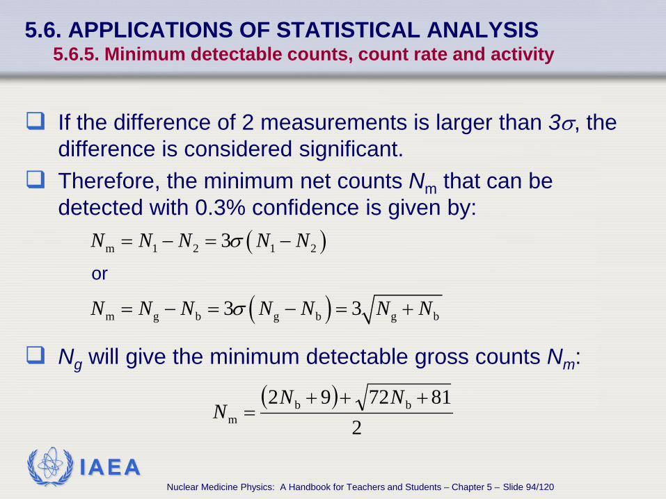
If the difference of 2 measurements is larger than 3σ, the difference is considered significant.

Therefore, the minimum net counts Nm that can be detected with 0.3% confidence is given by:

or

Ng will give the minimum detectable gross counts Nm:

( )

( )

m 1 2 1 2

m g b g b g b

3

3 3

N N N N N

N N N N N N N

σ

σ

= − = −

= − = − = +

( )2

817292 bbm

+++=

NNN


IAEA

5.6. APPLICATIONS OF STATISTICAL ANALYSIS 5.6.5. Minimum detectable counts, count rate and activity

An approximation can be used by assuming that Ng ≈ Nb and:

The minimum detectable activity Am can be calculated

where S is the sensitivity of the detection system (count rate per becquerel), t is the time that the background was counted

bbg 23 NNN +≈

tSNA m

m =


IAEA

5.6. APPLICATIONS OF STATISTICAL ANALYSIS 5.6.5. Minimum detectable counts, count rate and activity 5.6.5.1. Example: calculation of minimum activity that can be detected

A detector is to be used to detect 131I in thyroid of radiation workers • Nb = 441 counts • tb = 5 min • Acquisition time = 5 min • Counter sensitivity = 0.1 counts · s–1 · Bq–1 • What is the minimum activity that can be detected?

( )m

535 4413.124 Bq

5 60 0.1A

−= =

× ×

5352

8144172)94412(2

8172)92( bbg =

+×++×=

+++=

NNN

g b 94 countsN N− =This image cannot currently be displayed.


IAEA

The minimum detectable net count rate: • Nb = 441 counts • tb = 5 min • Acquisition time = 5 min • Counter sensitivity = 0.1 counts · s–1 · Bq–1 • What is the minimum activity that can be detected?

( )bgbgm 3 RRRRR −>−= σ

b bb 2

g g g bg

36 369 812

2

R RRt t t t

R

+ + + +

=

5.6. APPLICATIONS OF STATISTICAL ANALYSIS 5.6.5. Minimum detectable counts, count rate and activity 5.6.5.1. Example: calculation of minimum activity that can be detected


IAEA

5.6. APPLICATIONS OF STATISTICAL ANALYSIS 5.6.5. Minimum detectable counts, count rate and activity 5.6.5.2. Example 2: calculation of minimum activity that can be detected

Assuming that Rg ~ Rb:

The minimum detectable activity Am can be calculated:

b

b

g

bbg 3

tR

tRRR ++≈

SRA m

m =


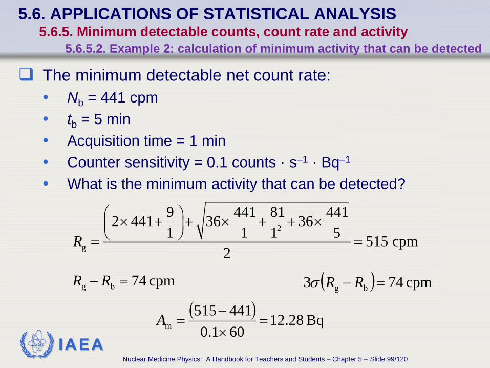
IAEA

The minimum detectable net count rate: • Nb = 441 cpm • tb = 5 min • Acquisition time = 1 min • Counter sensitivity = 0.1 counts · s–1 · Bq–1 • What is the minimum activity that can be detected?

cpm 74bg =− RR

2

g

9 441 81 4412 441 36 361 1 1 5 515 cpm

2R

× + + × + + × = =

( ) cpm 743 bg =− RRσ

( ) Bq 28.12601.0441515

m =×−

=A

5.6. APPLICATIONS OF STATISTICAL ANALYSIS 5.6.5. Minimum detectable counts, count rate and activity 5.6.5.2. Example 2: calculation of minimum activity that can be detected


IAEA

5.6. APPLICATIONS OF STATISTICAL ANALYSIS 5.6.6. Comparing counting systems

Important points:

• Large number of counts have smaller σF

• σF increases rapidly as Nb increases

• High sensitivity counting system with low background

• But as sensitivity increases the system will also be more

sensitive to background


IAEA


Analysis of sensitivity/background trade-off

• Compare results from systems 1 and 2 • t is the same for Ng and Nb

• σF for net sample counts obtained with the 2 systems are:

( )b1g1

b1g1S11F NN

NNN

−

+=σ ( )

b2g2

b2g2S2F2 NN

NNN

−

+=σ

( )( )

b2g2

b2g2

b1g1

b1g1

S2F2

S1F1

NNNN

NNNN

NN

−

+

−

+

=σσ


IAEA


System 1 is statistically the preferred system if:

System 2 is statistically the preferred system if:

( )( ) 1

S2F2

S1F1 <NN

σσ

( )( ) 1

S2F2

S1F1 >NN

σσ


IAEA


Systems can be compared using RS & σF for the count rate using the ratio of the σF's:

Use to compare different counting times in the same system for measuring fixed geometry samples

( )( )

b2g2

b2

b2

g2

g2

b1g1

b1

b1

g1

g1

S2F2

S1F1

RRtR

tR

RRtR

tR

RR

−

+

−

+

=σσ


IAEA


To obtain the best energy window selection in a system, or to compare 2 systems, the same t should be used:

Can also be used in planar imaging

Different collimators can be evaluated by comparing counts from a target region to a non-target or background region

Spatial resolution is also important and must be considered

( )( )

b2g2

b2g2

b1g1

b1g1

S2F2

S1F1

RRRR

RRRR

RR

−

+

−

+

=σσ


IAEA

5.6. APPLICATIONS OF STATISTICAL ANALYSIS 5.6.7. Estimating required counting times

Suppose • Want to determine Rs to within a certain σF(Rs)

• Suppose Rga & Rba are known from preliminary measurements • t is the same for the sample & background

• The time required to achieve the desired statistical reliability

( ) ( )ga ba

22F S ga ba

R Rt

R R Rσ

+=

−


IAEA

5.6. APPLICATIONS OF STATISTICAL ANALYSIS 5.6.7. Estimating required counting 5.6.7.1. Example: calculation of required counting time

Determine the counting time for a thyroid uptake study using a collimated detector • Preliminary target measurement of Rga = 900 cpm • Preliminary background Rba = 100 cpm • What counting time is required to determine the net count rate

to within 5%? • t = 0.625 min for both target & background • Total time =1.25 min

( ) ( ) ( ) ( )

min 625.080005.0

100010090005.0

1009002222 =

×=

−×+

=t

cpm 800100900sa =−=R


IAEA

Plasma volume (PV) and its uncertainty is to be measured using the dilution principle

• Procedure • Prepare plasma sample of known volume • Prepare standard sample with same activity & volume • Dilute standard sample and then count • Obtain blood sample 10 min after injection • Separate plasma from the blood • Count blood sample • Calculate PV by:

VDRR

p

sPV =

5.6. APPLICATIONS OF STATISTICAL ANALYSIS 5.6.8. Calculating uncertainties in the measurement of plasma volume in patients


IAEA


Using the values: • Counting time t = 10 min • V ± σP(V) = 5 ± 3% mL • D ± σP(D) = 200 ± 3% • Rs+b = 3200 cpm • Rp+b = 1200 cpm • Rb = 200 cpm

The uncertainties are calculated step by step by applying the propagation of errors:


IAEA


Using the expressions: • Standard sample net count rate per mL

• Rs = Rs+b – Rb; • Rb = background count rate • Rs+b = standard sample gross count rate per mL • Plasma sample net count rate per mL

• Rp = Rp+b – Rb; • Rp+b = plasma sample gross count rate per mL • V = volume of standard sample in mL • σP(V) = percentage uncertainty in V • D = dilution of standard sample • σP(D) = percentage uncertainty in D


IAEA



IAEA

5.7. APPLICATION OF STATISTICAL ANALYSIS: DETECTOR PERFORMANCE 5.7.1. Energy resolution of scintillation detect

Poisson statistics affect other aspects of the detection of radiation: • Determines detector energy resolution • Determines uncertainty of energy measurement of detected photon

Energy resolution / uncertainty determined by: • Detector type

e.g. solid state detector energy resolution significantly better than of scintillation detector

• Photon energy

Energy resolution for detector / radionuclide does not change between samples • Different from statistics uncertainty determined by number of counts

accumulated


IAEA


Even for the same sample and same detector system, the uncertainty can change if measurements are repeated following the decay of the nuclide

Another important consequence of statistics is that in scintillation cameras the location of the position of incoming photons is based on the pulses detected by the detectors

Therefore, the statistics of the detector system limits the spatial resolution that can be achieved with an imaging device. A clear understanding of the statistics associated with the detector when detecting a photon is, therefore, important


IAEA


The operation of scintillation detectors can be considered a three stage process:

• x = number of light photons produced in scintillator by detected gamma rays

• p = fraction of light photons that will eject electrons from the photocathode of the photomultiplier tube (PMT)

• M = multiplication electrons at successive dynodes before being collected at the anode


IAEA


Average number of electrons produced at the anode:

Fractional variance in the electron number N for a 3 stage cascade process:

For dynodes with identical M

Assuming the production of light photons follows a Poisson distribution:

xpMN =e

( ) ( ) ( ) ( )2 2 2 2F e F F FN x xp xpMσ σ σ σ= + +

( )2 11F M

Mσ =

−

( )x

x 12F =σ ( )

ppp −

=12

Fσ


IAEA


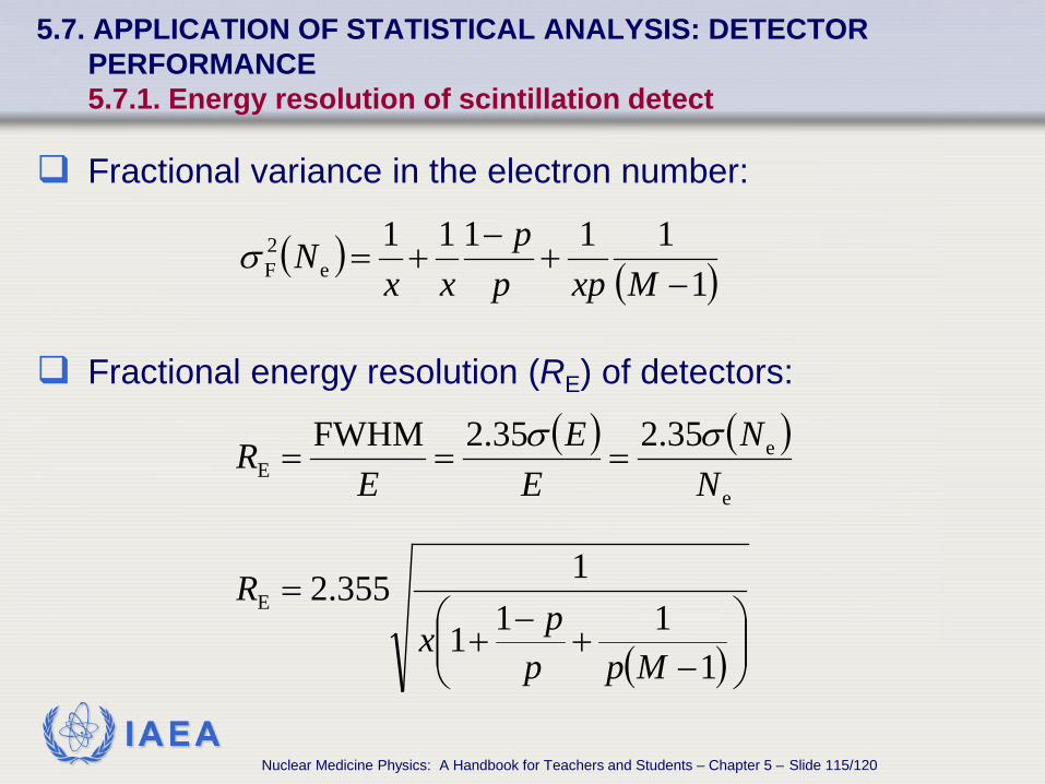
Fractional variance in the electron number:

Fractional energy resolution (RE) of detectors:

( ) ( )111111

e2F −

+−

+=Mxpp

pxx

Nσ

( ) ( )e

eE

35.235.2FWHMN

NE

EE

R σσ===

( )

−

+−

+=

1111

1355.2E

Mpppx

R


IAEA

5.7. APPLICATION OF STATISTICAL ANALYSIS: DETECTOR PERFORMANCE 5.7.2. Intervals between successive events

Calculation and measurement of the paralysable dead time of counting systems involves time intervals separating random events

• r = average rate at which events are occurring • rdt = differential probability for event taking place in the

differential time increment dt

For a radiation detector with unity efficiency, the time interval for counting a single radionuclide is given by:

NtNr λ==

dd


IAEA


To derive the distribution function to describe the time interval between adjacent random events

• Assume an event has occurred at t = 0

• Two independent processes must take place: • No events may occur within the time interval from 0 to t • An event must take place in the next differential time increment dt • Overall probability given by :

• P1(t) dt = Probability of next event taking place dt after delay of t • P(0) = Probability of number of events during time from 0 to t • r dt = Probability of event during dt

1( ) d (0) dP t t P r t= ×


IAEA


The possibility that no events will be recorded over an interval of t

• rt = average number of recorded events • Substituting

• Most probable distribution is zero • Average interval length:

( ) ( ) rtrtrtP −

−

== e!0e0

0

1(t)d e drtP t r t−=


IAEA

5.7. APPLICATION OF STATISTICAL ANALYSIS: DETECTOR PERFORMANCE 5.7.3. Paralysable dead time

Paralysable dead time model • τ = fixed dead time following each event during detector live period • Events occurring during τ

• Not recorded • Create another fixed dead time τ on the lost event • m = recorded rate of events

• identical to rate of occurrences of time intervals > τ between trues

• The probability of intervals > τ :

• Rate of occurrence m of such intervals :

• must be solved iteratively to calculate r from measurements of m and τ

e rm r τ−=

2 1( ) d ( ) d e rP t t P t t τ

τ

∞ −= =∫


IAEA

BIBLIOGRAPHY

BUSHBERG, J.T., SEIBERT, J.A., LEIDHOLDT, E.M., BOONE, J.M., The Essential Physics of Medical Imaging, Lippincott Williams and Wilkins, London (2002)

CHERRY, S.R., SORENSON, J.A., PHELPS, M.E., Physics in Nuclear

Medicine, Saunders, Los Angeles, CA (2003) DELANEY C.F.G., FINCH, E.C., Radiation Detectors, Clarendon Press, Oxford

(1992) KNOLL, G.F., Radiation Detection and Measurement, John Wiley and Sons,

New York (1989) NATIONAL ELECTRICAL MANUFACTURERS ASSOCIATION, Standards

Publication NU 1-2007, Performance Measurements of Gamma Cameras (2007)


Documents

Chapter 5: Statistics for Radiation Measurement · International Atomic Energy Agency ... Chapter 5: Statistics for ... 5.2.1.1. Data set as a list . Nuclear Medicine Physics: