Chapter 5

Synthesis Algorithms

5.1. Introduction

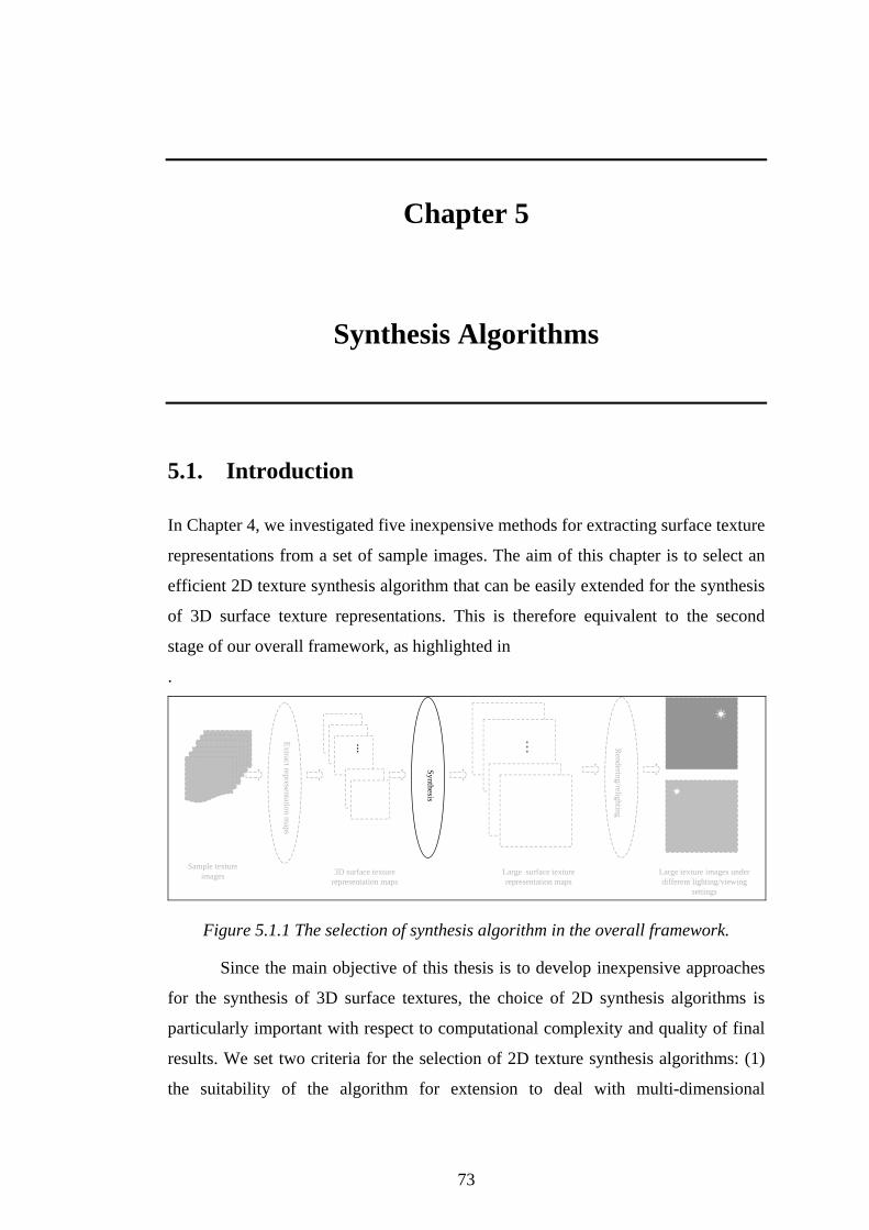
In Chapter 4, we investigated five inexpensive methods for extracting surface texture

representations from a set of sample images. The aim of this chapter is to select an

efficient 2D texture synthesis algorithm that can be easily extended for the synthesis

of 3D surface texture representations. This is therefore equivalent to the second

stage of our overall framework, as highlighted in

.

Sample textureimages

Extract representation maps

Synthesis

3D surface texturerepresentation maps

Large surface texturerepresentation maps

Rendering/relighting

Large texture images underdifferent lighting/viewing

settings

...

...

Figure 5.1.1 The selection of synthesis algorithm in the overall framework.

Since the main objective of this thesis is to develop inexpensive approaches

for the synthesis of 3D surface textures, the choice of 2D synthesis algorithms is

particularly important with respect to computational complexity and quality of final

results. We set two criteria for the selection of 2D texture synthesis algorithms: (1)

the suitability of the algorithm for extension to deal with multi-dimensional

73

representations, and (2) the capability of producing good results while requiring little

computation.

We first present a detailed survey of recent publications on 2D texture

synthesis. Then we investigate two popular approaches based on [Wei2000] and

[Efros2001] respectively. The first approach synthesises images from small sample

textures at pixel scale by employing a multi-resolution decomposition technique.

The second approach synthesises the result image by ‘stitching’ together small

patches selected from the sample image. We propose simple modifications to these

two methods, which can reduce the computation and produce similar synthesis

results to the originals. On comparing the two approaches, we select the modified

Efros’ 2D texture synthesis algorithm as our basic algorithm, as it can produce better

results while requiring less computation. In particular, we analyse the effects on

output images produced by varying the four input parameters of the selected

algorithm.

The rest of this chapter is organised as following. Section 5.2 presents a

detailed survey on 2D texture synthesis methods. Section 5.3 describes the two

selected approaches and compares them in terms of computational complexity and

quality of results. Section 5.4 analyses the input parameters of the selected

algorithm, and finally we conclude our work of this chapter in section 5.5.

5.2. A detailed survey of synthesis algorithms

The goal of this section is to survey 2D texture synthesis algorithms using the

criteria that we proposed in the previous section. In Chapter 2, we divided 2D

synthesis algorithms into two groups according to the sampling strategies.

Accordingly, this survey is also based on this taxonomy. Two algorithms are

selected for further investigation at the end of this section.

5.2.1. Texture synthesis methods based on global sampling

strategies

As discussed in Chapter 2, texture synthesis algorithms employing global sampling

strategies synthesise new images by matching global statistics between the sample

and result images in feature space. In general, these texture synthesis methods are

74

not preferable for the use of synthesising surface relighting representations in multi-

dimensional space. One reason is that the surface relighting representations normally

consist of multi-dimensional vectors with correlation existing between the elements.

For the synthesised surface representations, the correlation is unlikely to be

maintained during global sampling process. Meanwhile, these methods essentially

amount to a multi-parameter and non-linear optimisation process over a single

image. As shown in Table 2.1.1, two typical methods [Zhu2000 and Portilla200],

which produced good synthesis results over a wide range of sample textures, require

more than 20 minutes for computing. Extending these approaches to multi-

dimensional surface representations would require iteration and optimisation over

inter as well as intra image parameters. Consequently, the computation may be

expensive.

Many 2D texture synthesis methods synthesise result images by matching

marginal or joint histograms between the sample and result images [Heeger1995,

Van Nevel 1998, Zhu2000 and Copeland2001]. For 3D surface texture synthesis, the

input consists of multi-dimensional vectors that represent the sample surface texture

under arbitrary illumination. Thus, the one-dimensional histograms in 2D texture

synthesis algorithms will become multi-dimensional histograms in 3D surface

texture synthesis. During the matching process, the element values of the result

multi-dimensional vectors are changed according to the sample histograms. This

might destroy the correlation between the surface relighting representations. For

example, if we use surface gradients and albedo maps as the representation of a

Lambertian surface, the matching process will change the result surface gradients

and albedo values by purely comparing the sample and result histograms. In order to

maintain the relighting characteristics, the interrelationship [e.g. cross correlation

between components (elements)] of the multi-dimensional data must be kept for an

iteration method. This results in a complex multi-dimensional optimisation problem.

Meanwhile, if the number of bins is large or the dimensionality is high, there might

be too few pixels in each bin for a multi-dimensional histogram. For instance, if we

calculate a six-dimensional histogram using six 64x64 representation maps and each

dimension is divided into 10 bins, we only have, on average, 6*64*64/106=0.025

pixels in each bin. Thus, it is difficult to accurately estimate the multi-dimensional

75

histograms. A similar problem might exist in those methods that synthesise new

images by matching various statistics, e.g. [Jacovitti1998, Portilla2000 and

Campisi2002].

In general, 2D synthesis algorithms that employ global sampling strategies

become more complex when being extended to use multi-dimensional vectors as

input. The method proposed in [Eom1998] estimates the parameters of a 2D moving

model; it would be more difficult if implemented in high dimensional space.

Although De Bonet’s method can be easily extended to take surface relighting

representations in multi-dimensional space as input, it is not clear whether the filter

bank is sufficient to capture the characterisations of the sample representations [De

Bonet1997].

To summarise:

Two-dimensional texture synthesis algorithms that employ global sampling

strategies are generally not suitable as the basis of algorithms in 3D surface texture

synthesis approaches. The main reason is that these algorithms become too complex

or have difficulty to preserve the correlation between surface relighting

representations when they are extended to multi-dimensional space.

5.2.2. Texture synthesis methods based on local sampling strategies

As introduced in Chapter 2, texture synthesis methods based on local sampling

strategies synthesise new images by matching local information between the sample

and result images. These methods can be further divided into two sub-classes

depending on whether they employ a parametric and non-parametric model.

In general, parametric methods require expensive computation due to the

estimation of the parameters. Zhu et. al. estimate the parameters of the FRAME

model for texture synthesis; they report that the computational cost increases

proportionally with the size of the filter window and long iterations are required to

achieve accuracy [Zhu1995]. Bader et. al. implement parallel algorithms for the

synthesis in order to reduce the computing time [Bader1995]. Zhang et. al. estimate

the parameters of the wavelet autoregressive model and the radial basis function

network for modelling and synthesising texture images [Zhang1998b]. Their

multiresolution AR model has a total of 91 parameters. If multi-dimensional surface

76

representations are used as input in these methods, both the models and the

computation become more complex.

Non-parametric texture synthesis methods are less complex compared with

their parametric counterparts because they do not need to estimate the parameters of

statistical models [Efros1999, Wei2000, Hertzmann2001, Efros2001, Parada2001,

Ashikhmin2001, Harrison2001, Tonietto2002, Zelinka2002, Cohen2003

Nealen2003, Paget1998, Ashlock1999, Bar-Joseph2001, Xu2001, Liang2001 and

Gousseau2002]. Thus, these methods are more suitable for extension to use multi-

dimensional representations as input. However, several methods still require

expensive computation. Paget and Longstaff require parallel algorithms for the

synthesis using non-causal, non-parametric and multiscale Markov random field

[Paget1998]. Ashlock and Davidson apply tandem generic algorithms for texture

synthesis based on non-parametric partially ordered Markov models; their method

need several hours to compute [Ashlock1999]. On the other hand, recent non-

parametric synthesis approaches have been reported to be able to produce good

results with less computation [Efros1999, Wei2000, Bar-Joseph2001, Xu2001,

Liang2001, Hertzmann2001, Efros2001, Ashikhmin2001, Harrison2001,

Tonietto2002, Zelinka2002, Cohen2003 and Nealen2003]. In these approaches, pixel

values in the synthesised results are obtained from the sample images. The

correlation between synthesised surface representations can be kept. Therefore, these

methods are more suitable for the synthesis of surface relighting representations in

multi-dimensional space. In particular, several patch-based synthesis algorithms

([Efros2001, Xu2001 and Liang2001]) have one of the smallest requirements in

terms of computational complexity.

The algorithm proposed in [Efros1999] is a highlight in the research field of

texture synthesis. It assumes a Markov random field model and calculates the

conditional distribution of a pixel given all its neighbours by querying the sample

image and finding all similar neighbourhoods. The conditional probability density

function can be estimated using the following set: )|),((RNresult IyxIp

}*)1(* :{)),(( mindIIGIIyxIRss NNsampleNresult ε+≤−⊂=Ψ (5.2.1)

where:

77

),( yxIresult is the intensity value of the pixel (x, y) to be synthesised in the

output result image

is the neighbourhood centred at pixel (x, y) in the output image RNI

is a neighbourhood in the input sample image SNI

)(*SR NN IIG − is a weighted Sum of Squared Differences (SSD) by a

Gaussian kernel G between pixel values in an sample neighbourhood and

the result neighbourhood , which is centred at

sN

RN ),( yxIresult

mind is the minimum SSD between pixel values in the input and the output

neighbourhood, weighted by a Gaussian kernel G

ε is the error threshold and is set to 0.1

The centred pixel values of neighbourhoods in )),(( yxIresultΨ provide an estimated

histogram for . Thus, the algorithm first finds the best-matched

neighbourhoods (within certain error tolerance

),( yxIresult

ε ) in the sample image for the result

neighbourhood centred by . Then a best-matched neighbourhood is

randomly selected and its centred pixel value is assigned to . Although

the algorithm is simple and not fast, it can produce promising synthesis results.

Based on this algorithm, Wei and Levoy employed image pyramid representations to

develop a new synthesis algorithm and used the tree-structured vector quantization

for acceleration [Wei2000].

RN ),( yxIresult

),( yxIresult

The work in [Efros1999 and Wei2000] has received broad attention in the

computer vision and computer graphics communities. Later work based on these two

algorithms includes [Ashikhmin2001, Hertzmann2001, Efros2001, Parada2001,

Tonietto2002, Zelinka2002, Cohen2003 and Nealen2003]. In [Ashikhmin2001],

Ashikhmin modifies the algorithm of [Wei2000] and achieves faster synthesis

speeds, which allow direct user input for interactive control over the synthesis

process. In [Hertzmann2001], Hertzmann et. al. propose an image processing

framework called image analogies, which can learn the analogy between the original

and filtered input images to produce new image pairs. Their algorithm is based on

[Wei2000 and Ashikmin2001]. In [Parada2001], Parada and Ruiz-del-Solar use self-

organizing maps to improve the algorithm of [Wei2000]. In [Efros2001], Efros and

78

Freeman develop a patch-based texture synthesis algorithm, which is based on

[Efros1999] but produces better results with much less computation. In

[Tonietto2002], a local-controlled synthesis algorithm is proposed that can generate

texture in which the basic elements have different sizes, e.g. the skin of a cheetah. In

[Zelinka2002], a jump map is first generated to store the matching input pixels and

then used to synthesise a new texture image in real-time. In [Cohen2003], Wang

tiles are employed and combined with the algorithm of [Efros2001] for texture

synthesis. In [Nealen2003], a pixel-based algorithm and a patch-based algorithm are

combined to improve previous synthesis methods.

To summarise:

Since estimating the parameters of statistical models in multi-dimensional

space is complex, parametric texture synthesis methods with local sampling

strategies are not suitable for synthesising multi-dimensional surface relighting

representations. On the other hand, most non-parametric synthesis approaches can be

easily extended to dealing with multi-dimensional representations, and they can

produce good results with little computation. Thus, we select two non-parametric

texture synthesis approaches based on [Wei2000 and Efros2001] for future

investigation.

5.2.3. Summary

We have surveyed 2D texture synthesis approaches using the two criteria: (1) the

suitability of the algorithm for extension to deal with multi-dimensional

representations, and (2) the capability of producing good results while requiring little

computation. Texture synthesis algorithms employing global sampling strategies

have difficulty to synthesise the multi-dimensional surface representations because

they tend to become excessively complex, and the correlation between the result

representations may be damaged. On the other hand, non-parametric synthesis

algorithms with local sampling strategies are capable of taking multi-dimensional

vectors as input and producing good results with less computation. We therefore

select two non-parametric approaches based on [Wei2000 and Efros2001] as

candidate basic algorithms for 3D surface texture synthesis.

79

5.3. Two Approaches

This section investigates two 2D texture synthesis approaches based on [Wei2000]

and [Efros2001].

5.3.1. The first approach and modification—a pixel-based multi-

resolution approach

The first approach employs a pixel-based multi-resolution texture synthesis

algorithm, which is based on a non-parametric sampling method [Wei2000]. The

algorithm in [Wei2000] can be seen as the extension of the work in [Efros1999]. It

also assumes a Markov random field texture model, which means a pixel value at a

certain location only depends on its immediate neighbourhood. If we recall the

expression (5.2.1), the algorithm in [Wei2000] essentially uses neighbourhoods

across different resolutions and synthesises pixel values from lower to higher

resolutions incrementally. The size of the neighbourhood is a parameter of the

algorithm and must be chosen taking into account the granularity of the subject

texture. When choosing the value of the next pixel in the output image the algorithm

uses the populated portion of the pixel’s neighbourhood to exhaustively search for

the ‘best’ matched region in the sample image.

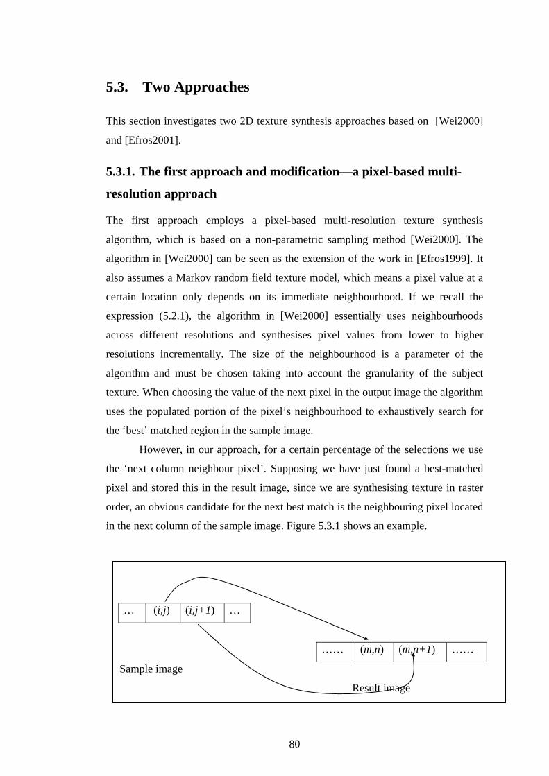
However, in our approach, for a certain percentage of the selections we use

the ‘next column neighbour pixel’. Supposing we have just found a best-matched

pixel and stored this in the result image, since we are synthesising texture in raster

order, an obvious candidate for the next best match is the neighbouring pixel located

in the next column of the sample image. Figure 5.3.1 shows an example.

… (i,j) (i,j+1) …

…… (m,n) (m,n+1) ……

Sample image

Result image

80

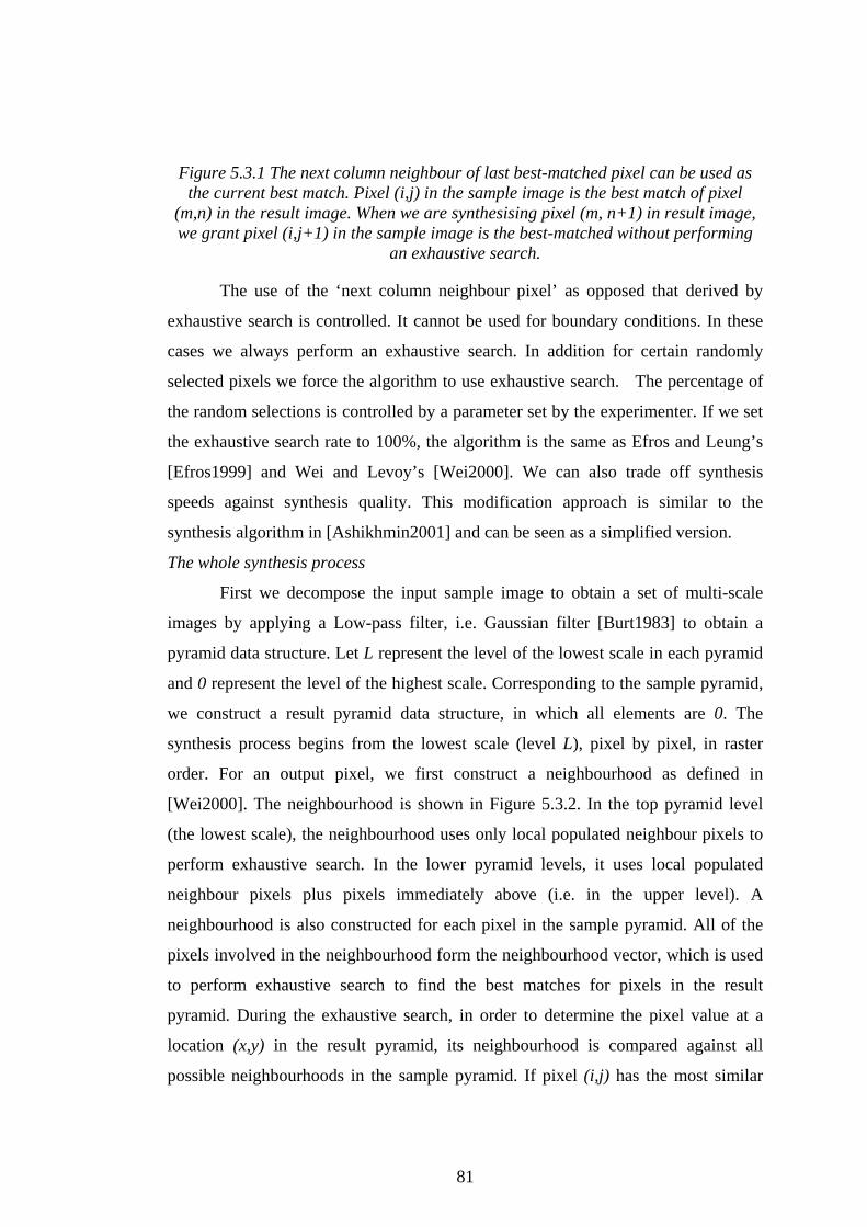
Figure 5.3.1 The next column neighbour of last best-matched pixel can be used as the current best match. Pixel (i,j) in the sample image is the best match of pixel

(m,n) in the result image. When we are synthesising pixel (m, n+1) in result image, we grant pixel (i,j+1) in the sample image is the best-matched without performing

an exhaustive search.

The use of the ‘next column neighbour pixel’ as opposed that derived by

exhaustive search is controlled. It cannot be used for boundary conditions. In these

cases we always perform an exhaustive search. In addition for certain randomly

selected pixels we force the algorithm to use exhaustive search. The percentage of

the random selections is controlled by a parameter set by the experimenter. If we set

the exhaustive search rate to 100%, the algorithm is the same as Efros and Leung’s

[Efros1999] and Wei and Levoy’s [Wei2000]. We can also trade off synthesis

speeds against synthesis quality. This modification approach is similar to the

synthesis algorithm in [Ashikhmin2001] and can be seen as a simplified version.

The whole synthesis process

First we decompose the input sample image to obtain a set of multi-scale

images by applying a Low-pass filter, i.e. Gaussian filter [Burt1983] to obtain a

pyramid data structure. Let L represent the level of the lowest scale in each pyramid

and 0 represent the level of the highest scale. Corresponding to the sample pyramid,

we construct a result pyramid data structure, in which all elements are 0. The

synthesis process begins from the lowest scale (level L), pixel by pixel, in raster

order. For an output pixel, we first construct a neighbourhood as defined in

[Wei2000]. The neighbourhood is shown in Figure 5.3.2. In the top pyramid level

(the lowest scale), the neighbourhood uses only local populated neighbour pixels to

perform exhaustive search. In the lower pyramid levels, it uses local populated

neighbour pixels plus pixels immediately above (i.e. in the upper level). A

neighbourhood is also constructed for each pixel in the sample pyramid. All of the

pixels involved in the neighbourhood form the neighbourhood vector, which is used

to perform exhaustive search to find the best matches for pixels in the result

pyramid. During the exhaustive search, in order to determine the pixel value at a

location (x,y) in the result pyramid, its neighbourhood is compared against all

possible neighbourhoods in the sample pyramid. If pixel (i,j) has the most similar

81

neighbourhood, the value of pixel (i,j) in the sample pyramid is assigned to pixel

(x,y) in the result pyramid. We use the Sum of Absolute Differences (SAD) to

measure the similarity between neighbourhoods. More details about the exhaustive

search algorithm can be found in [Wei2000].

P P P P PP P P P PP P X P P P

P Y PP P P

l l+1

Figure 5.3.2. The neighbourhood defined by Wei and Levoy [Wei2000]. The current level of pyramid “l” is shown at left and the upper level “l+1” is shown at right. It

uses local populated neighbour pixels (marked as “P” in level “l”) plus pixels immediate above in the upper level (marked as “P” in level “l+1”). All of marked pixels form the sub-neighbourhood. The current output pixel is marked as X, which locates at (x, y) in the lth pyramid level. Its “parent” pixel in the l+1 pyramid level locates at (x/2, y/2), which is marked as Y. Since the level “l+1” is complete, this sub-neighbourhood can contain all pixels around Y. The sub-neighbourhood is

constructed for each sample pyramid and result pyramid.

We use the ‘next column neighbour pixel’ as the best-matched pixel

whenever allowed. Now suppose we have synthesised the pixel located at (m,n) in

level X (X<=L), and its best-matched pixel locates at (k,l) in level X of the sample

pyramid. Let {X, (m, n)} represent the pixel location in the result pyramid and {X, (k,

l)} for the pixel location of the sample pyramid. We are going to find the best match

for next pixel. Suppose the next pixel locates at {X, (m, n+1)} of the result pyramid.

Intuitively, we consider the next column neighbour pixel of {X, (k, l)} in the sample

pyramid as the candidate of the best match of pixel {X, (m, n+1)}. If {X, (k, l+1)}

exists in the sample pyramid, we grant the neighbourhood of {X, (k, l+1)} as the best

match for that of {X, (m, n+1)} in the result pyramid. The pixel value of {X, (k, l+1)}

of the sample pyramid is assigned to the pixel value of {X, (m, n+1)} of the result

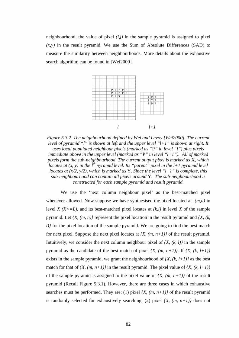
pyramid (Recall Figure 5.3.1). However, there are three cases in which exhaustive

searches must be performed. They are: (1) pixel {X, (m, n+1)} of the result pyramid

is randomly selected for exhaustively searching; (2) pixel {X, (m, n+1)} does not

82

exist in the result pyramid, which means {X, (m, n)} is the last pixel of the mth row;

and (3) pixel {X, (k, l+1)} of the sample pyramid does not exist. Figure 5.3.3 shows

these three cases.

The synthesis process will continue until all pixels in the result pyramid are

assigned values from the lowest scale to the highest scale. In the highest scale (level

0), the required result image is synthesised. The pseudocode is shown in Table 5.3.1.

For most textures, the ratio of exhaustive search is from 40% to 70% given good

results. The quality of synthesis results is similar to previous work by using 100%

exhaustive search [Wei2000][Efros1999], but the computational complexity is

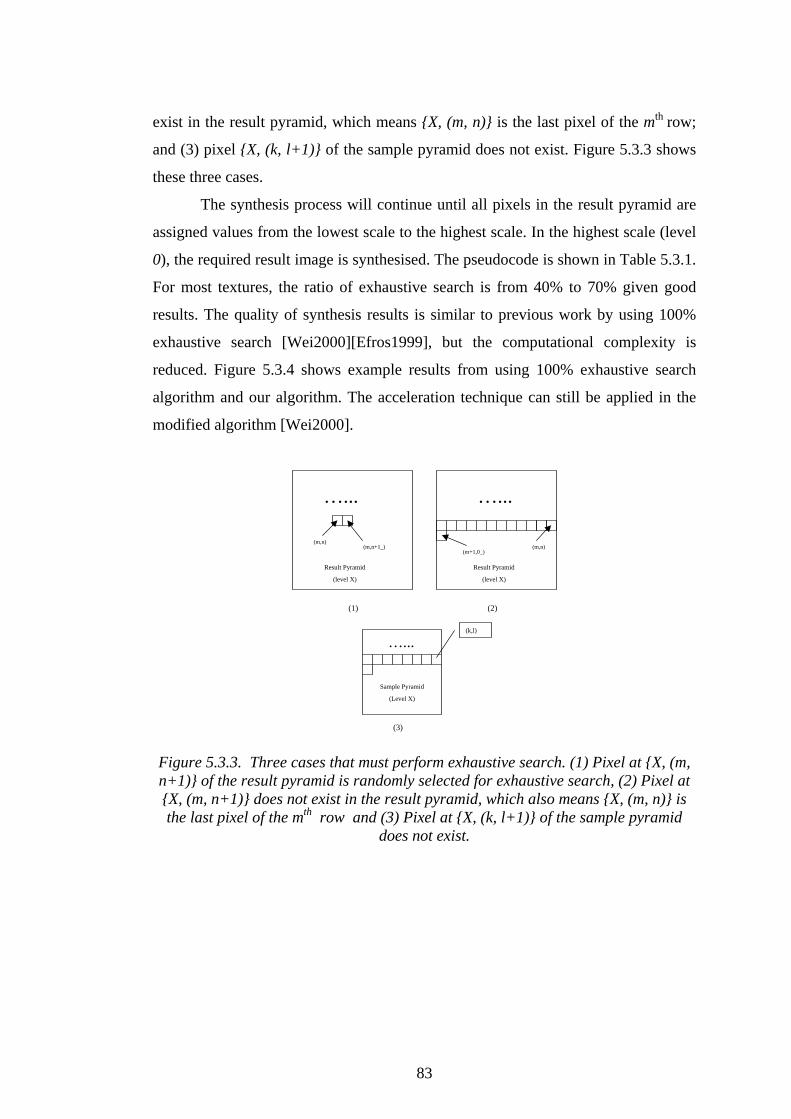
reduced. Figure 5.3.4 shows example results from using 100% exhaustive search

algorithm and our algorithm. The acceleration technique can still be applied in the

modified algorithm [Wei2000].

(k,l)

(m,n)(m,n+1_) (m,n)

(m+1,0_)

Result Pyramid

(level X)

Result Pyramid

(level X)

…...…...

Sample Pyramid

(Level X)

…...

(1)

(3)

(2)

Figure 5.3.3. Three cases that must perform exhaustive search. (1) Pixel at {X, (m, n+1)} of the result pyramid is randomly selected for exhaustive search, (2) Pixel at {X, (m, n+1)} does not exist in the result pyramid, which also means {X, (m, n)} is the last pixel of the mth row and (3) Pixel at {X, (k, l+1)} of the sample pyramid

does not exist.

83

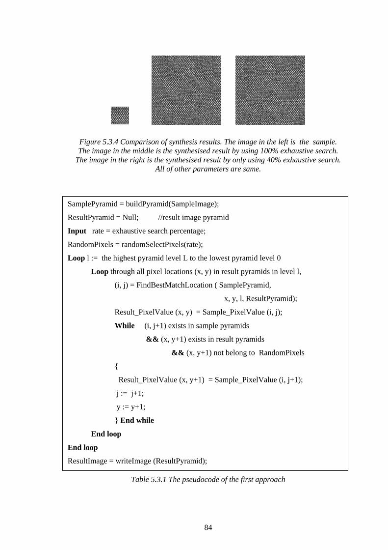
Figure 5.3.4 Comparison of synthesis results. The image in the left is the sample. The image in the middle is the synthesised result by using 100% exhaustive search.

The image in the right is the synthesised result by only using 40% exhaustive search. All of other parameters are same.

SamplePyramid = buildPyramid(SampleImage);

ResultPyramid = Null; //result image pyramid

Input rate = exhaustive search percentage;

RandomPixels = randomSelectPixels(rate);

Loop l := the highest pyramid level L to the lowest pyramid level 0

Loop through all pixel locations (x, y) in result pyramids in level l,

(i, j) = FindBestMatchLocation ( SamplePyramid,

x, y, l, ResultPyramid);

Result_PixelValue (x, y) = Sample_PixelValue (i, j);

While (i, j+1) exists in sample pyramids

&& (x, y+1) exists in result pyramids

&& (x, y+1) not belong to RandomPixels

{

Result_PixelValue (x, y+1) = Sample_PixelValue (i, j+1);

j := j+1;

y := y+1;

} End while

End loop

End loop

ResultImage = writeImage (ResultPyramid);

Table 5.3.1 The pseudocode of the first approach

84

To summarise:

We have investigated a 2D texture synthesis approach proposed by

[Wei2000]. It assumes a Markov Random Field texture model, which means a pixel

value at a certain location only depends on its immediate neighbourhood. A multi-

resolution scheme is applied to construct the neighbourhood around a given pixel.

The algorithm synthesises a result image in pixel scale by finding the best-matched

neighbourhoods in the sample image. We modified the original algorithm by using

the ‘next column neighbour pixel’ as the best-matched pixel for a certain percentage

of pixel locations. The modification can produce similar results with less

computation.

5.3.2. The second approach and modification—A patch-based

approach

The second approach is based on the image quilting method proposed by Efros and

Freeman [Efros2001]. The method synthesises a new image by ‘stitching’ together

small patches from the sample image. It requires little computation and can produce

remarkable synthesis results. This method is also an extension of the previous work

in [Efros1999].

The method in [Efros2001] synthesises a result image block by block in

raster order. Square blocks are used to capture the primary pattern in the sample

texture. The size of the block is a parameter of the algorithm and must be chosen

taking into account the granularity of the subject texture. First, a block is randomly

selected from the sample image and pasted into the new image beginning at the first

row and the first column. Then another block is selected as a candidate neighbour. It

is placed next to the first block so that they overlap one another. The overlapping

area between the two blocks is used to test the goodness of fit of the candidate using

an L2 norm (Sum of Squared Differences). This is repeated for different candidates

to find the minimum difference metric (distance). The final neighbour is randomly

selected from those blocks whose distance lies in a certain range of the minimum

distance. The range is controlled by a predefined error tolerance. A minimum error

boundary cut is calculated in the overlapping area between the overlapping pixels so

that the boundary looks smooth, as shown in Figure 5.3.5. Both vertical and

85

horizontal overlapping areas are used for selecting best-matched blocks inside the

new image. This whole process is repeated until an output image of the required size

has been generated.

We have made two modifications to this quilting algorithm. First, instead of

locating the best-matched block using exhaustive search, we select the ‘next column

neighbour block’, which is the corresponding neighbour of last selection, and assign

it as the current best-matched block, providing it exists in the sample image. This

modification is similar to that introduced for the first approach. During the synthesis

process, after a best-matched block is found in the sample image, we store its

location in an array. When a new block in the result image is being synthesised, we

check the best-matched block locations of its already generated neighbours. If there

exists a block that is adjacent to all the best-matched block locations in the sample

image, this block is selected as the current best-matched block. Figure 5.3.6

illustrates this process. Suppose we are going to synthesise block h’ in the result

image. We first check the best-matched blocks of its existing neighbour blocks e’, f’

and g’. If their best-matched blocks e, f and g are adjacent in the sample image, then

block h, which is the neighbour of e, f and g, is selected as the best-matched block

for h’. Obviously, for the first block row or column in the result image, only one

neighbour block is checked. This simplification can increase the speed of the

algorithm without apparently affecting the output. It can also be seen as an extension

of the method used in [Ashikhmin2001].

The second modification to the original algorithm is that we use an error

metric based on the Sum of Absolute Differences (SAD) rather than more expensive

L2 norm (square of SAD). They produced similar results in our experiments.

Although both the L2 norm and the SAD are not perfect as perceptual metrics, the

existing perceptual metrics might not be completely reliable and require more

expensive computations [Sebe2000, Bolin1998, Ramasubramania1999 and

Ashikhmin2001]. Figure 5.3.7 shows example output images produced by the

modified and original algorithms respectively. The pseudocode of the whole

algorithm is listed in Table 5.3.2.

86

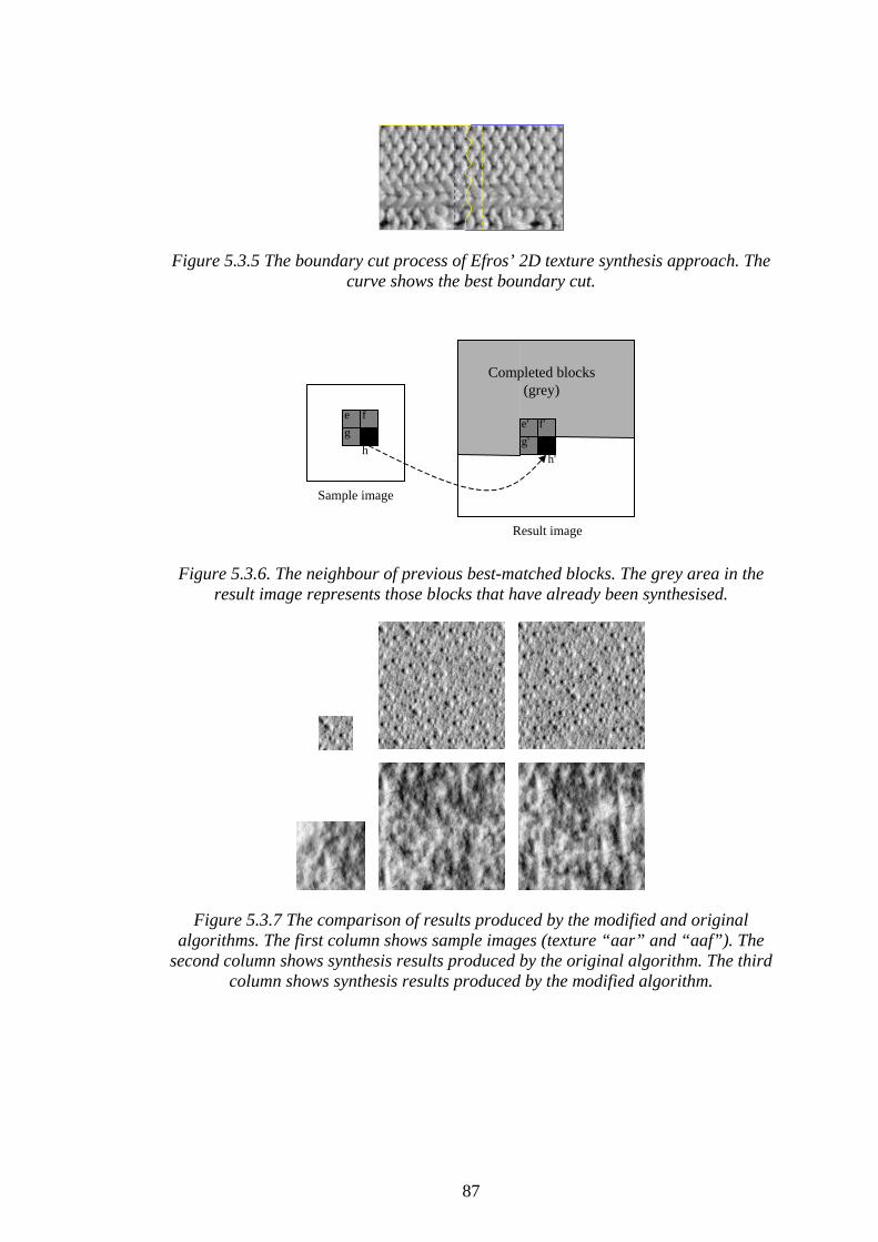
Figure 5.3.5 The boundary cut process of Efros’ 2D texture synthesis approach. The curve shows the best boundary cut.

e fg

hh'

f'e'g'

Sample image

Result image

Completed blocks(grey)

Figure 5.3.6. The neighbour of previous best-matched blocks. The grey area in the result image represents those blocks that have already been synthesised.

Figure 5.3.7 The comparison of results produced by the modified and original algorithms. The first column shows sample images (texture “aar” and “aaf”). The

second column shows synthesis results produced by the original algorithm. The third column shows synthesis results produced by the modified algorithm.

87

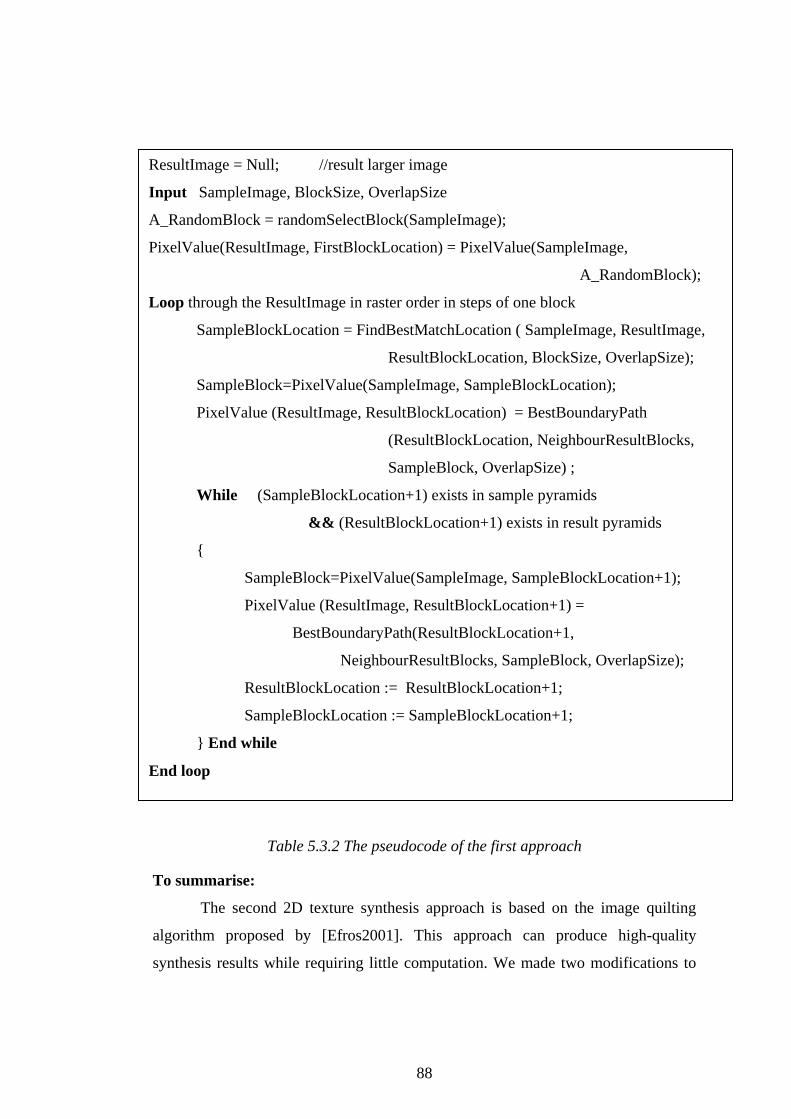
ResultImage = Null; //result larger image

Input SampleImage, BlockSize, OverlapSize

A_RandomBlock = randomSelectBlock(SampleImage);

PixelValue(ResultImage, FirstBlockLocation) = PixelValue(SampleImage,

A_RandomBlock);

Loop through the ResultImage in raster order in steps of one block

SampleBlockLocation = FindBestMatchLocation ( SampleImage, ResultImage,

ResultBlockLocation, BlockSize, OverlapSize);

SampleBlock=PixelValue(SampleImage, SampleBlockLocation);

PixelValue (ResultImage, ResultBlockLocation) = BestBoundaryPath

(ResultBlockLocation, NeighbourResultBlocks,

SampleBlock, OverlapSize) ;

While (SampleBlockLocation+1) exists in sample pyramids

&& (ResultBlockLocation+1) exists in result pyramids

{

SampleBlock=PixelValue(SampleImage, SampleBlockLocation+1);

PixelValue (ResultImage, ResultBlockLocation+1) =

BestBoundaryPath(ResultBlockLocation+1,

NeighbourResultBlocks, SampleBlock, OverlapSize);

ResultBlockLocation := ResultBlockLocation+1;

SampleBlockLocation := SampleBlockLocation+1;

} End while

End loop

Table 5.3.2 The pseudocode of the first approach

To summarise:

The second 2D texture synthesis approach is based on the image quilting

algorithm proposed by [Efros2001]. This approach can produce high-quality

synthesis results while requiring little computation. We made two modifications to

88

the original algorithm. The modified algorithm can produce similar results to those

from original algorithm while the computation is reduced.

5.3.3. Comparison of the two approaches

In section 5.3.2, we investigated two 2D texture synthesis approaches. Since the

main goal of this thesis is to develop inexpensive approaches for the synthesis of 3D

surface texture, we need to select one method which requires less computation while

producing reasonable results. Therefore, we first compare the two approaches

according to the computational complexity and synthesis results.

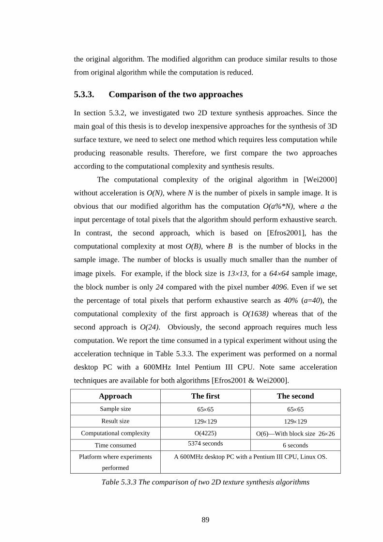
The computational complexity of the original algorithm in [Wei2000]

without acceleration is O(N), where N is the number of pixels in sample image. It is

obvious that our modified algorithm has the computation O(a%*N), where a the

input percentage of total pixels that the algorithm should perform exhaustive search.

In contrast, the second approach, which is based on [Efros2001], has the

computational complexity at most O(B), where B is the number of blocks in the

sample image. The number of blocks is usually much smaller than the number of

image pixels. For example, if the block size is 13×13, for a 64×64 sample image,

the block number is only 24 compared with the pixel number 4096. Even if we set

the percentage of total pixels that perform exhaustive search as 40% (a=40), the

computational complexity of the first approach is O(1638) whereas that of the

second approach is O(24). Obviously, the second approach requires much less

computation. We report the time consumed in a typical experiment without using the

acceleration technique in Table 5.3.3. The experiment was performed on a normal

desktop PC with a 600MHz Intel Pentium III CPU. Note same acceleration

techniques are available for both algorithms [Efros2001 & Wei2000].

Approach The first The second Sample size 65×65 65×65

Result size 129×129 129×129

Computational complexity O(4225) O(6)—With block size 26×26

Time consumed 5374 seconds 6 seconds

Platform where experiments

performed

A 600MHz desktop PC with a Pentium III CPU, Linux OS.

Table 5.3.3 The comparison of two 2D texture synthesis algorithms

89

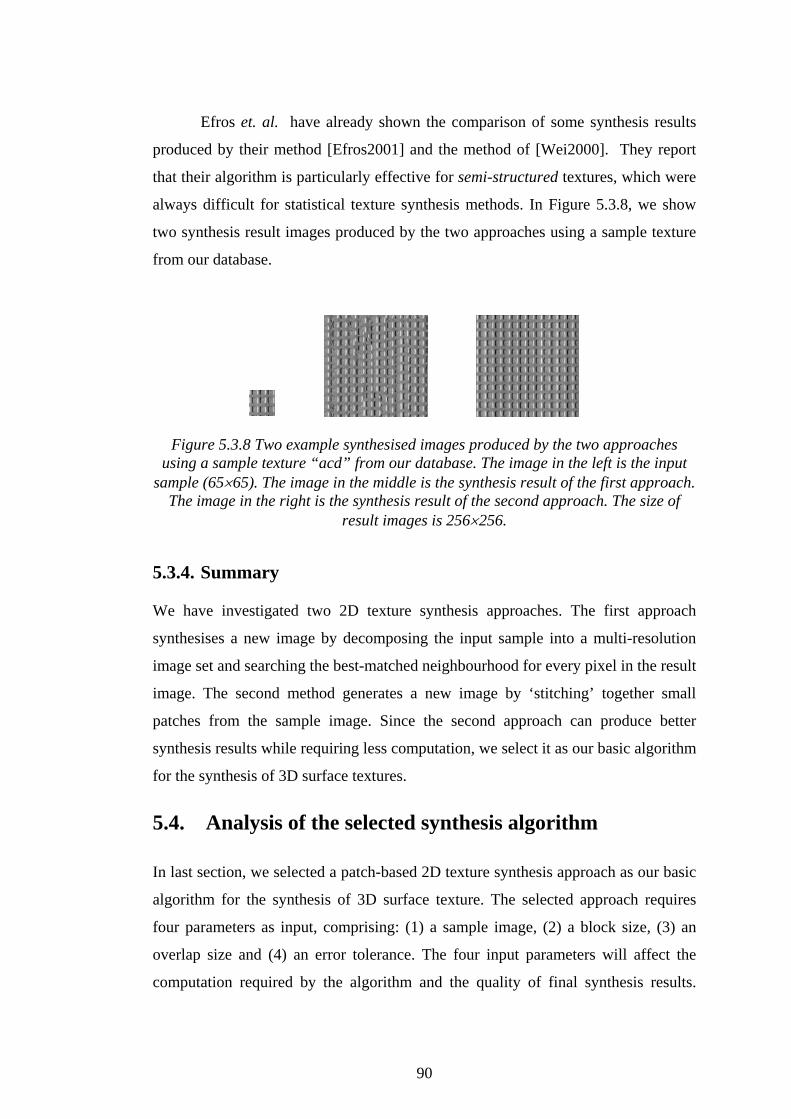
Efros et. al. have already shown the comparison of some synthesis results

produced by their method [Efros2001] and the method of [Wei2000]. They report

that their algorithm is particularly effective for semi-structured textures, which were

always difficult for statistical texture synthesis methods. In Figure 5.3.8, we show

two synthesis result images produced by the two approaches using a sample texture

from our database.

Figure 5.3.8 Two example synthesised images produced by the two approaches using a sample texture “acd” from our database. The image in the left is the input

sample (65×65). The image in the middle is the synthesis result of the first approach. The image in the right is the synthesis result of the second approach. The size of

result images is 256×256.

5.3.4. Summary

We have investigated two 2D texture synthesis approaches. The first approach

synthesises a new image by decomposing the input sample into a multi-resolution

image set and searching the best-matched neighbourhood for every pixel in the result

image. The second method generates a new image by ‘stitching’ together small

patches from the sample image. Since the second approach can produce better

synthesis results while requiring less computation, we select it as our basic algorithm

for the synthesis of 3D surface textures.

5.4. Analysis of the selected synthesis algorithm

In last section, we selected a patch-based 2D texture synthesis approach as our basic

algorithm for the synthesis of 3D surface texture. The selected approach requires

four parameters as input, comprising: (1) a sample image, (2) a block size, (3) an

overlap size and (4) an error tolerance. The four input parameters will affect the

computation required by the algorithm and the quality of final synthesis results.

90

These effects are very important to the synthesis of 3D surface textures. This section

will therefore analyse the algorithm in terms of computation and synthesis results by

varying the input parameters.

5.4.1. Sample image size

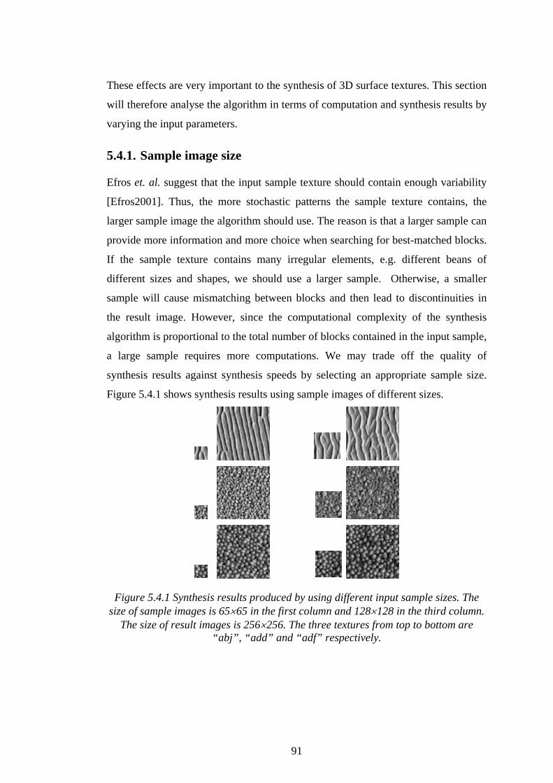
Efros et. al. suggest that the input sample texture should contain enough variability

[Efros2001]. Thus, the more stochastic patterns the sample texture contains, the

larger sample image the algorithm should use. The reason is that a larger sample can

provide more information and more choice when searching for best-matched blocks.

If the sample texture contains many irregular elements, e.g. different beans of

different sizes and shapes, we should use a larger sample. Otherwise, a smaller

sample will cause mismatching between blocks and then lead to discontinuities in

the result image. However, since the computational complexity of the synthesis

algorithm is proportional to the total number of blocks contained in the input sample,

a large sample requires more computations. We may trade off the quality of

synthesis results against synthesis speeds by selecting an appropriate sample size.

Figure 5.4.1 shows synthesis results using sample images of different sizes.

Figure 5.4.1 Synthesis results produced by using different input sample sizes. The size of sample images is 65×65 in the first column and 128×128 in the third column.

The size of result images is 256×256. The three textures from top to bottom are “abj”, “add” and “adf” respectively.

91

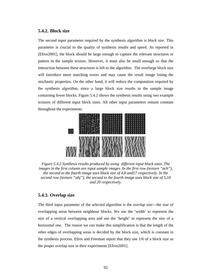
5.4.2. Block size

The second input parameter required by the synthesis algorithm is block size. This

parameter is crucial to the quality of synthesis results and speed. As reported in

[Efros2001], the block should be large enough to capture the relevant structures or

pattern in the sample texture. However, it must also be small enough so that the

interaction between these structures is left to the algorithm. The overlarge block size

will introduce more matching errors and may cause the result image losing the

stochastic properties. On the other hand, it will reduce the computation required by

the synthesis algorithm, since a large block size results in the sample image

containing fewer blocks. Figure 5.4.2 shows the synthesis results using two example

textures of different input block sizes. All other input parameters remain constant

throughout the experiments.

Figure 5.4.2 Synthesis results produced by using different input block sizes. The images in the first column are input sample images. In the first row (texture “ach”),

the second to the fourth image uses block size of 4,8 and17 respectively. In the second row (texture “abj”), the second to the fourth image uses block size of 5,10

and 20 respectively.

5.4.3. Overlap size

The third input parameter of the selected algorithm is the overlap size—the size of

overlapping areas between neighbour blocks. We use the ‘width’ to represent the

size of a vertical overlapping area and use the ‘height’ to represent the size of a

horizontal one. The reason we can make this simplification is that the length of the

other edges of overlapping areas is decided by the block size, which is constant in

the synthesis process. Efros and Freeman report that they use 1/6 of a block size as

the proper overlap size in their experiments [Efros2001].

92

Inappropriate overlap sizes will cause faulty matching during synthesis

which will introduce discontinuities in the synthesis results. The reason is that pixels

in overlapping areas are used for searching for the best-matched blocks. The

algorithm calculates Sum of Absolute Differences (SAD) using those pixels in the

overlapping areas; a block with the minimum SAD will be selected as the best-

matched block. If the overlap size is too small or too large, there are either too few

or too many pixels that can be used to calculate SAD. In either case, the minimum

SAD might not represent the real best-matched blocks due to the sum effect. For

example, suppose the best synthesis results are achieved by using a size that leads to

each overlapping area containing 200 pixels. For each block location, the algorithm

calculates

∑=

Ω′′−

200

1}),(),({min

iiiiij j

yxIyxI (5.4.1)

where:

jΩ is the overlapping area containing 200 pixels covered by block j in the

sample image and the already synthesised pixels in the result image

),( ii yx represents the ith pixel in the sample image covered by the

overlapping area jΩ

),( ii yx ′′ represents the ith pixel in the result image covered by the overlapping

area jΩ

is the i),( ii yxI th pixel value in the sample image

is the i),( ii yxI ′′′ th pixel value in the result image.

Suppose another overlap size that makes the overlapping area contain 600 pixels.

Then the following statement is not guaranteed to hold:

∑∑=

Ω′=

Ω′′′′′′−′′′′=′′−

600

1

200

1

}),(),({min}),(),({mini

iiiijiiiiij jj

yxIyxIyxIyxI (5.4.2)

where:

jΩ′ is the overlap area containing 600 pixels covered by block j in the

sample image and the already synthesised pixels in the result image

93

),( ii yx ′′′′ represents the ith pixel in the sample image covered by the

overlapping area jΩ′

),( ii yx ′′′′′′ represents the ith pixel in the result image covered by the overlapping

area jΩ′

is the i),( ii yxI ′′′′ th pixel value in the sample image

),( ii yxI ′′′′′′′ is the ith pixel value in the result image.

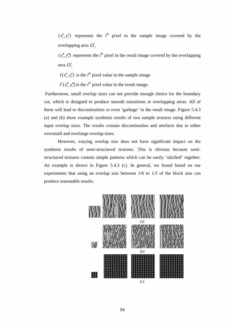
Furthermore, small overlap sizes can not provide enough choice for the boundary

cut, which is designed to produce smooth transitions in overlapping areas. All of

these will lead to discontinuities or even ‘garbage’ in the result image. Figure 5.4.3

(a) and (b) show example synthesis results of two sample textures using different

input overlap sizes. The results contain discontinuities and artefacts due to either

oversmall and overlarge overlap sizes.

However, varying overlap size does not have significant impact on the

synthesis results of semi-structured textures. This is obvious because semi-

structured textures contain simple patterns which can be easily ‘stitched’ together.

An example is shown in Figure 5.4.3 (c). In general, we found based on our

experiments that using an overlap size between 1/6 to 1/3 of the block size can

produce reasonable results.

(b)

(a)

(c)

94

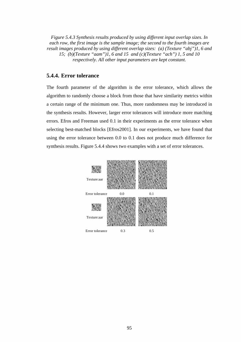
Figure 5.4.3 Synthesis results produced by using different input overlap sizes. In each row, the first image is the sample image; the second to the fourth images are

result images produced by using different overlap sizes: (a) (Texture “abj”)1, 6 and 15; (b)(Texture “aam”)1, 6 and 15 and (c)(Texture “ach”) 1, 5 and 10

respectively. All other input parameters are kept constant.

5.4.4. Error tolerance

The fourth parameter of the algorithm is the error tolerance, which allows the

algorithm to randomly choose a block from those that have similarity metrics within

a certain range of the minimum one. Thus, more randomness may be introduced in

the synthesis results. However, larger error tolerances will introduce more matching

errors. Efros and Freeman used 0.1 in their experiments as the error tolerance when

selecting best-matched blocks [Efros2001]. In our experiments, we have found that

using the error tolerance between 0.0 to 0.1 does not produce much difference for

synthesis results. Figure 5.4.4 shows two examples with a set of error tolerances.

Texture:aar

Error tolerance 0.0 0.1

Error tolerance 0.3 0.5

Texture:aar

95

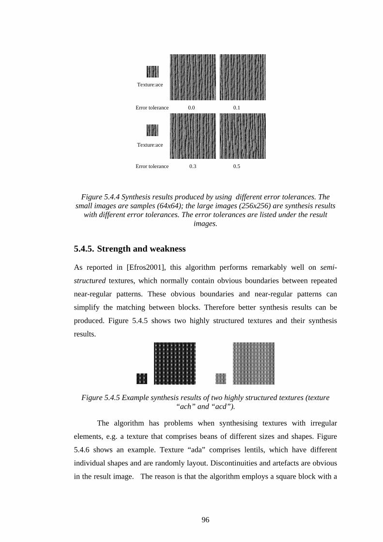
Texture:ace

Error tolerance 0.0 0.1

Error tolerance 0.3 0.5

Texture:ace

Figure 5.4.4 Synthesis results produced by using different error tolerances. The small images are samples (64x64); the large images (256x256) are synthesis results

with different error tolerances. The error tolerances are listed under the result images.

5.4.5. Strength and weakness

As reported in [Efros2001], this algorithm performs remarkably well on semi-

structured textures, which normally contain obvious boundaries between repeated

near-regular patterns. These obvious boundaries and near-regular patterns can

simplify the matching between blocks. Therefore better synthesis results can be

produced. Figure 5.4.5 shows two highly structured textures and their synthesis

results.

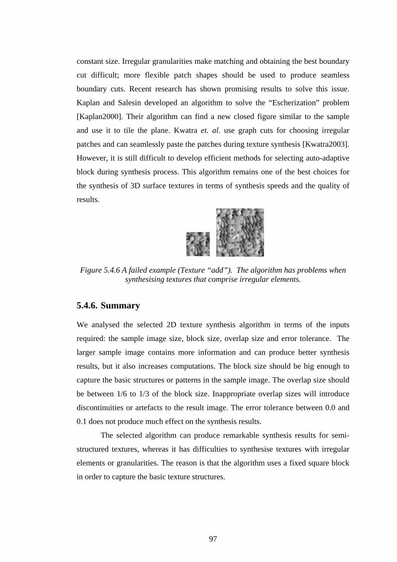
Figure 5.4.5 Example synthesis results of two highly structured textures (texture “ach” and “acd”).

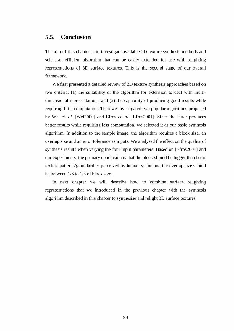
The algorithm has problems when synthesising textures with irregular

elements, e.g. a texture that comprises beans of different sizes and shapes. Figure

5.4.6 shows an example. Texture “ada” comprises lentils, which have different

individual shapes and are randomly layout. Discontinuities and artefacts are obvious

in the result image. The reason is that the algorithm employs a square block with a

96

constant size. Irregular granularities make matching and obtaining the best boundary

cut difficult; more flexible patch shapes should be used to produce seamless

boundary cuts. Recent research has shown promising results to solve this issue.

Kaplan and Salesin developed an algorithm to solve the “Escherization” problem

[Kaplan2000]. Their algorithm can find a new closed figure similar to the sample

and use it to tile the plane. Kwatra et. al. use graph cuts for choosing irregular

patches and can seamlessly paste the patches during texture synthesis [Kwatra2003].

However, it is still difficult to develop efficient methods for selecting auto-adaptive

block during synthesis process. This algorithm remains one of the best choices for

the synthesis of 3D surface textures in terms of synthesis speeds and the quality of

results.

Figure 5.4.6 A failed example (Texture “add”). The algorithm has problems when synthesising textures that comprise irregular elements.

5.4.6. Summary

We analysed the selected 2D texture synthesis algorithm in terms of the inputs

required: the sample image size, block size, overlap size and error tolerance. The

larger sample image contains more information and can produce better synthesis

results, but it also increases computations. The block size should be big enough to

capture the basic structures or patterns in the sample image. The overlap size should

be between 1/6 to 1/3 of the block size. Inappropriate overlap sizes will introduce

discontinuities or artefacts to the result image. The error tolerance between 0.0 and

0.1 does not produce much effect on the synthesis results.

The selected algorithm can produce remarkable synthesis results for semi-

structured textures, whereas it has difficulties to synthesise textures with irregular

elements or granularities. The reason is that the algorithm uses a fixed square block

in order to capture the basic texture structures.

97

5.5. Conclusion

The aim of this chapter is to investigate available 2D texture synthesis methods and

select an efficient algorithm that can be easily extended for use with relighting

representations of 3D surface textures. This is the second stage of our overall

framework.

We first presented a detailed review of 2D texture synthesis approaches based on

two criteria: (1) the suitability of the algorithm for extension to deal with multi-

dimensional representations, and (2) the capability of producing good results while

requiring little computation. Then we investigated two popular algorithms proposed

by Wei et. al. [Wei2000] and Efros et. al. [Efros2001]. Since the latter produces

better results while requiring less computation, we selected it as our basic synthesis

algorithm. In addition to the sample image, the algorithm requires a block size, an

overlap size and an error tolerance as inputs. We analysed the effect on the quality of

synthesis results when varying the four input parameters. Based on [Efros2001] and

our experiments, the primary conclusion is that the block should be bigger than basic

texture patterns/granularities perceived by human vision and the overlap size should

be between 1/6 to 1/3 of block size.

In next chapter we will describe how to combine surface relighting

representations that we introduced in the previous chapter with the synthesis

algorithm described in this chapter to synthesise and relight 3D surface textures.

98