85

CHAPTER 5

VEGETATION CLASSIFICATION USING SPACE-BORNE SAR DATA

5.1 INTRODUCTION:

Remote sensing techniques aided with ground information provide a

reliable source of vegetation classification in a cost and time-effective way.

While the utility of optical data in vegetation classification is well known, the

potential of airborne and space-borne radar systems is attempted

successfully in several studies. Radar sensors operating in different

wavelengths and polarizations can be widely used for large-scale land cover

mapping and monitoring using backscatter coefficients in different

polarizations and wavelength bands. C-band space borne SAR is widely

used for the classification of the vegetation type using techniques viz.,

texture measures, multi-sensor fusion, multi-polarization data, multi-

temporal data and polarimetric data (Strozzi et al., 2000; Rignot et al., 1997;

Nezry et al., 1993; Saatchi et al., 1997; Oliver, 1998; Frery et al., 1999;

Grover et al., 1999; Yanasse et al., 1997; Saatchi et al., 2000; Kimball et al.,

2004).

In the present study, three different approaches/ techniques were

discussed for vegetation classification using amplitude space-borne SAR

86

data in two wavelength bands; C-band ENVISAT-ASAR and L-band ALOS-

PALSAR datasets.

5.2 TECHNIQUES USED FOR VEGETATION CLASSIFICATION:

In the present study, vegetation classification using space-borne SAR

data was carried out using following techniques in C and L wavelength

bands:

5.2.1 First order statistics based vegetation classification

5.2.1 Multi-sensor fusion based vegetation classification

5.2.3 Texture measures based vegetation classification

5.2.1 First order statistics based vegetation classification:

Acquired ASAR and PALSAR data were preprocessed and calibrated to

backscattering coefficient and used for vegetation classification.

Backscattering coefficient of different land use classes were analysed using

the ground truth points; mean, standard deviation and range of

backscattering coefficient for each land cover class is calculated. Using

these values, thresholdings of backscattering coefficient for each land cover

class is determined and applied on images for vegetation classification.

5.2.1.1 Using dual polarization ASAR data: The FCC combination of

dual polarized data i.e., HH and VV; VV and VH enabled the discrimination

of vegetated and non-vegetated areas but the delineation within the

vegetated areas i.e., forest and agriculture was unclear. Basic land cover

87

types viz., vegetation, non-vegetation areas, settlements and water bodies

were discriminated from the dual-polarized ASAR data. Settlements showed

high backscattering coefficient values, followed by barren/fallow lands and

then by vegetation. Backscattering coefficient of water is very low.

Backscattering coefficient of agriculture and forested areas were in the same

range and hence could not be discriminated. Though mean backscattering

coefficient of agriculture and forested areas are different, there was an

overlap in the standard deviation of range of values. Hence, the

discrimination of vegetation classes using backscattering coefficient of ASAR

data was not clear. The use of multi-temporal data ENVISAT-ASAR data

may be useful for discrimination of forest and agriculture.

5.2.1.2 Using ALOS-PALSAR data: Backscattering coefficient of

different land use classes were analyzed from the pixel values belonging to

ground truth points of particular class. Different vegetation classes have

different backscattering coefficient values and hence, discrimination of

vegetation classes was carried out with the thresholding of backscatter

coefficient values for each land cover class.

From the fig 5.1, it can be seen that the backscattering coefficients of

moist-deciduous forests, teak forests, agriculture, barren and water are

different.

88

ALOS-PALSAR showed the clear discrimination of forest, teak forests,

agriculture, barren and water bodies. The backscattering coefficient of

forested area is high followed by agriculture and then by barren lands (Fig

5.2 (a)).

Teak plantations within the forested area were discernable as their

backscattering coefficient is greater than the forested area. This may be

attributed to the systematic arrangement of trees, similar height class and

age of the trees. The forested area in terrain appeared bright and saturated

in the image. The shadow regions were misclassified as crops. This may be

due to low backscattering coefficient in the shadow regions which is in same

range with backscattering coefficient of agriculture.

Fig 4.1: Variation of backscattering coefficient of PALSAR data in different landuse classes

-20

-16

-12

-8

-4

0

Water Barren Agriculture MDforest Teak

Back

scat

terin

g co

effic

ient

(dB)

Land Use classes

Variation in backscattering coeficient of PALSAR data in different landuse classes

89

Accuracy assessment of the classified map (Fig 5.2 (b)) was carried out by

generating error matrix and kappa statistics. Accuracy assessment points in

the classified image were generated stratified randomly and the accuracy

assessment was carried out comparing with ground truth points and IRS P6

LISS-III image. Overall classification accuracy and kappa statistics using

stand alone PALSAR single polarization data was 82.4% and 0.72

respectively and the details are given in table 5.1. Discrimination of barren

areas with current fallow was not proper. The cropped area is discernable

but crop harvested area and current fallow regions were classified as

barren/non-vegetated areas. The discrimination within forested areas was

enhanced and classification accuracy/discrimination capability was better

than ASAR data.

Fig 5.2: (a) L-band PALSAR HH polarized data (b) Classified image of Achanakmar-Amarkantak Biosphere Reserve,Bilaspur

Teak dominated forest Moist deciduous forest Forested area in terrainCrop land WaterNon-vegetated area

a bTeak dominated forest Moist deciduous forest Forested area in terrainCrop land WaterNon-vegetated areaTeak dominated forest Moist deciduous forest Forested area in terrainCrop land WaterNon-vegetated area

a b

90

Table 5.1: Accuracy assessment and Kappa statistics of classified map generated from first order statistics

Class name Producer's accuracy User's accuracy Kappa statistics

Non-vegetated area 83.33% 71.43% 0.82

Mixed moist deciduous forest 78.57% 73.33% 0.69

Teak dominated forest 75.00% 60.00% 0.57

Cropland 84.21% 84.21% 0.81 Water 90.91% 76.92% 0.74

However, backscattering coefficient values also depend on the phyllotaxy,

physiognomy, canopy structure and different species compositions present

in the study area hence the use of multi-sensor fusion and texture

measures based vegetation classification enhance the classification

capability of SAR data.

5.2.2 Multi-sensor fusion based vegetation classification

5.2.2.1 Introduction: Studies on the fusion of microwave and optical

data have shown the enhanced capabilities of merged data for improved

delineation of LULC categories. Image fusion techniques deal with

integration of complementary and redundant information from multiple

images to create a composite image that contains a better description of the

scene (Saraf et al., 1999). Data fusion can reduce the uncertainty associated

with the data acquired by different sensors or by same sensor with temporal

variation. Further, the fusion techniques may improve interpretation

capabilities with respect to subsequent tasks by using complementary

information sources (Wen and Chen, 2004).

91

The fusion of two data sets can be done in order to obtain one single data

set with the qualities of both (Saraf et al., 1999). The low-resolution

multispectral satellite imagery can be combined with the higher resolution

radar imagery by fusion technique to improve the interpretability of the

merged image. The resultant data product has the advantages of high

spatial resolution, structural information (from radar image), and spectral

resolution (from optical and infrared bands). Thus, the merged image

provides faster interpretation (Simone et al., 2002), and can help in

extracting more features (Wen and Chen, 2004).Various image fusion

techniques viz., Intensity-Hue-Saturation, Principal component analysis,

Bovey transformation, Wavelet transformation etc., are available in

published literature (Li et al., 2002; Tu et al., 2001). Image fusion improves

geometric corrections, classification accuracy, substitutes missing

information; enhance certain features (Pohl, 1996).

5.2.2.2 Methodology: The potential of the fusion of SAR data with

optical data for discrimination of different land-cover classes in parts of

Dandeli sub division, Uttara Kannada district, Western Ghats, Karnataka,

India (Refer Chapter-3 for detail description of the study area) was carried

out in the present study. Environment Satellite’s (ENVISAT) C-band

Advanced Synthetic Aperture Radar (ASAR) data of 30 Oct 2006 with HH

polarization and Advanced Land Observing Satellite (ALOS) – Phased Array

L-band Synthetic Aperture Radar (PALSAR) data of 10th Feb 2007 with HH

polarization were merged with Indian Remote Sensing Satellite – Linear

92

Imaging Self Scanning Sensor-III (IRS-P6 LISS-III) data collected on 11 Jan

2006 were used for vegetation classification.

The schematic diagram for generation of vegetation classified map from

multi-sensor fusion technique is given in fig 5.3.

The backscatter images of ASAR and PALSAR in HH polarization were

merged with LISS-III data using Intensity Hue Saturation technique, as IHS

technique is considered as standard procedure in image analysis. The IHS is

a colour related technique which effectively separates spatial (I) and spectral

(H, S) information from a standard RGB image.

IHS colour transformation based image fusion is one of the standard

methods for sharpening of multi-sensor data. The hue value corresponds to

Fig 5.3: Methodology flow chart for multi-sensor fusion

Spaceborne SAR data IRS P6 LISS-III data

Preprocessing of SAR data Atmospheric correction

Geocoding, Co-registration, Resampling to common grid

Intensity, hue, saturation fusion technique

Supervised classification

Vegetation classification

93

the dominant wavelength of the light, saturation is a colour’s purity and

intensity measures the brightness of a colour. The three components of the

original image R, G and B are transformed into the IHS colour space. After

the transformation, the low-resolution intensity component I is replaced by

the SAR band with higher spatial resolution, the final step is to transform

the image back to RGB colour space with the original values of H and S

(Pohl, 1996). The mathematical description and RGB to IHS is given below:

5.2.2.3 Mathematical description: The IHS colour transformation

effectively separates spatial (I) and spectral (H, S) information from a

standard RGB image. From the equation below, I relates to the intensity,

while `v1’ and `v2’ represent intermediate variables which are needed in the

transformation. H and S stand for Hue and Saturation, (Harrison and Jupp,

1990; Pohl, 1996).

⎟⎟⎟

⎠

⎞

⎜⎜⎜

⎝

⎛

⎟⎟⎟⎟⎟⎟⎟

⎠

⎞

⎜⎜⎜⎜⎜⎜⎜

⎝

⎛

−

−=⎟⎟⎟

⎠

⎞

⎜⎜⎜

⎝

⎛

BGR

vvI

02

12

16

26

16

13

13

13

1

.2

1 ----------- (5.1)

⎟⎟⎠

⎞⎜⎜⎝

⎛= −

1

21tanvvH -------- (5.2) 2

221 vvS += -------- (5.3)

IHS technique transforms three channels of the data set representing

RGB into the IHS colour space which separates the colour aspects in its

94

average brightness (intensity). IHS technique replaces one of the three

components (I, H or S) of one data set with another image (Pohl, 1996).

Reverse transformation from IHS to RGB is given in below equation which

converts the data into its original image space to obtain the fused image

(Hinse and Proulx, 1995; Pohl, 1996).

⎟⎟⎟

⎠

⎞

⎜⎜⎜

⎝

⎛

⎟⎟⎟⎟⎟⎟⎟

⎠

⎞

⎜⎜⎜⎜⎜⎜⎜

⎝

⎛

−

−=⎟⎟⎟

⎠

⎞

⎜⎜⎜

⎝

⎛

2

1

06

23

12

16

13

12

16

13

1

. vvI

BGR

--------------- (5.4)

The merged data of ASAR and PALSAR were subjected to supervised

classification using maximum likelihood classifier, by giving training areas

based on ground-based information, and the accuracy assessment of the

classified outputs has been carried out by generating confusion matrices

and kappa statistics.

5.2.2.4 Results and Discussion: The fused C-band and L-band images

were generated and Vegetation classified maps were generated for the study

area. Accuracy assessments of classified maps were carried out.

95

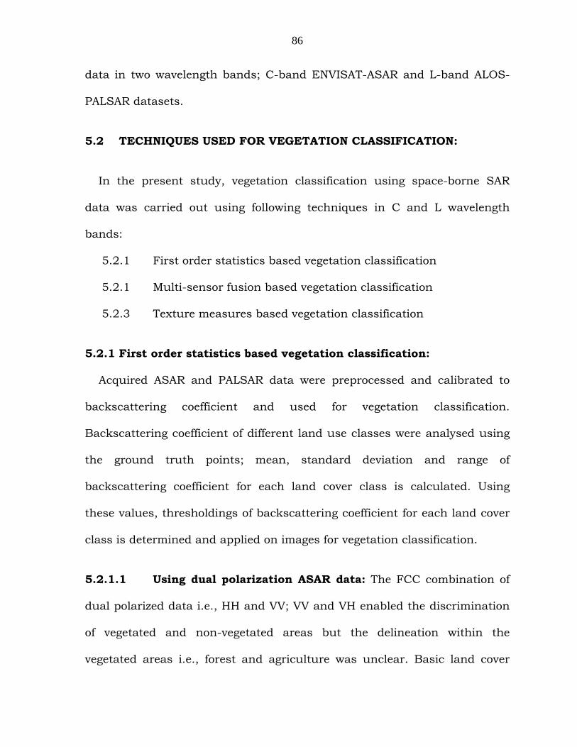
2.2.4.1 Using C-band ENVISAT-ASAR data: The merged output has

been found to delineate the forest types better apart from other land-cover

classes and minimize the shadow effect when compared with the stand

alone ASAR backscattering coefficient threshold.

Fig 5.4: FCC of IHS merged data for Dandeli site, Karnataka

96

ASAR images contributed different signals due to differences in surface

roughness, shape and moisture content of the observed ground cover. And

the optical data rely on the spectral signature of the ground targets in the

image.

Fig 5.5: Vegetation classified map of IHS merged data for Dandeli site

Settlements

97

Therefore, fusion of optical and microwave data (fig 5.4) provided a

unique combination that enhanced the identification of classes, forest

classification (Fig 5.5).

The classification accuracy of remote sensing images was improved when

fused data was used for deriving information on vegetation classification.

The overall classification accuracy and kappa coefficient of ASAR merged

data was 84% and 0.77 respectively and is given in table 5.2. Fused data

provided robust operational performance, i.e., increased confidence, reduced

ambiguity, improved reliability and improved classification (Rogers and

Wood, 1990).

Table 5.2: Accuracy assessment and Kappa statistics of classified map generated from ASAR merged data

Class name Producer's accuracy User's accuracy

Kappa statistics

Water 90.91% 89.21% 0.86 Mixed moist deciduous 73.75% 78.24% 0.74 Teak 75.23% 72.34% 0.71 Agriculture 76.47% 86.67% 0.79 Barren 66.67% 66.67% 0.62

Fused image enhanced the classification capability within the forests.

Teak forests could be clearly discriminated in the fused image. There was

clear distinction between forested and agricultural areas in the merged

image. The LISS-III image enabled not only discrimination of various land

cover types but also delineation of sub categories of forest types in the

merged data.

98

2.2.4.2 Using L-band ALOS-PALSAR data:

FCC of merged PALSAR data bands discriminated forest, agriculture,

water and barren areas. Within forest, the differentiation of teak forests and

mixed moist deciduous forests was possible. The results were in accordance

with the ASAR merged data. However, the discrimination of small patches of

teak plantation within the forested areas (Fig 5.6) was possible using

merged PALSAR data. The differentiation of the teak plantation in C-band

merged was not possible as the resolution of C-band ASAR used was coarser

and thus were not able to differentiate in merged C-band data.

Classified map generated from maximum likelihood supervised

classification technique discriminated water, agriculture, moist deciduous

forests, teak mixed forests and barren lands. Accuracy assessment of the

classified map was carried out by generating error matrix and kappa

statistics. The overall classification accuracy and kappa statistics were 83%

and 0.76 respectively and are given in table 5.3.

(a) L-BAND ALOS-PALSAR (b) FCC OF IRSP6-LISS-III (c) MERGED DATA OF PALSAR AND LISS-III(a) L-BAND ALOS-PALSAR (b) FCC OF IRSP6-LISS-III (c) MERGED DATA OF PALSAR AND LISS-III(a) L-BAND ALOS-PALSAR (b) FCC OF IRSP6-LISS-III (c) MERGED DATA OF PALSAR AND LISS-III(a) L-BAND ALOS-PALSAR (b) FCC OF IRSP6-LISS-III (c) MERGED DATA OF PALSAR AND LISS-III

Fig 5.6: Delineation of teak plantations in forested area of Dandeli site (yellow colour represents teak plantation).

99

However, barren lands with low backscattering coefficient and some

shadow regions were misclassified as water bodies. The forested area in

rough terrain regions was also misclassified. This may be due to high

backscatter coefficient from the slopes facing the sensor. The PALSAR

merged data gave better differentiation of teak plantations within the

vegetation when compared to the ASAR merged data. This may be attributed

to the resolution of the sensor and penetration capability which depends on

the sensor.

Table 5.3: Accuracy assessment and Kappa statistics of classified map generated from PALSAR merged data

Class name Producer's accuracy

User's accuracy

Kappa statistics

Water 92.59% 89.29% 0.81 Agriculture 80.00% 85.71% 0.81 Barren 83.33% 71.43% 0.71 Mixed moist deciduous forest 66.67% 75.00% 0.68 Teak forest 66.67% 66.67% 0.65

The analysis and results lay emphasis on the potential of multi-source

fusion of SAR data with optical data in discriminating different vegetation

types. SAR data can contribute significantly towards better classification

results when used in conjunction with optical RS data. However, the

constraints in the level of classification techniques when used exclusively

with respect to forested areas can be overcome with the use of multi-

frequency and polarimetric data.

100

5.2.3 Texture measures based vegetation classification:

As our objective was vegetation classification using stand-alone SAR data

and to utilize the maximum application potential of ASAR data in vegetation

classification, texture measures were computed and used in the present

study.

5.2.3.1 Introduction: Various studies showed that texture is the most

important source of information in high-resolution radar images (Ulaby et

al., 1982; Dobson et al., 1995; Dellacqua et al., 2003; Vander Saden, 1997).

Texture can be defined as the various measures of smoothness, coarseness,

and regularity of an image region (Rogers and Woods, 1992). The popular

grey-level co-occurrence matrix (GLCM) texture model (Haralick et al., 1973)

has been widely used in remote sensing studies (Clausi, 2002; Franklin et

al., 2001; Ouma et al., 2008). Recently, texture-based classification

algorithms have been successfully applied to VHR satellite imagery (Aguera

et al., 2008; Ouma et al., 2008; Puissant et al., 2005).

The grey level co-occurrence matrix or GLCM (Haralick et al., 1973;

Parker, 1997; Shapiro and Stockman, 2001) is one of the most widely used

texture measures, and was first suggested as a mechanism for deriving

texture measures by Haralick et al., (1973). Texture analysis in SAR data

was considered as the most important source of information (Luckman et

al., 1997) and textural measures were considered for automated land cover

classification. Luckman et al., (1997) were able to qualitatively distinguish

101

between three regeneration stages, using CCRS Convair 580 C-band data

over the Brazilian Amazon.

Measuring texture in images using the grey level co-occurrence matrix

(GLCM) has been carried out in few studies (Collins et al., 2000, Marceau et

al., 1990). Maillard, (2003) and Dulyakarn et al., (2000) compared texture

analysis methods and suggested Grey Level Co-occurrence Matrix (GLCM)

as the effective texture analysis scheme. Haralick et al., (1973) proposed

several measures that can be used to extract useful textural information

from a GLCM. GLCM is a measure of the probability of occurrence of two

grey levels separated by a given distance in a given direction (Mather, 1999).

As the GLCM is calculated for a given pixel separation, it is sensitive to the

scale and directionality of image texture. It also requires that the horizontal

and vertical offsets of the two pixels be specified along with the size of image

segment over which the GLCM should be constructed by a moving window

of a given size.

Many researches explained texture measures using GLCM matrix (Barber

and LeDrew, 1991, Soh et al., 1999; Roneorp et al., 1998) for variety of

applications like land-cover mapping (Kurosu et al., 1999; Vander Sanden

and Hoekman, 1999; Wu and Linders, 1999), crop discrimination (Soares et

al., 1997) and forest studies (Luckman et al., 1997; Kurvonen et al., 1999;

Van der Sanden and Hoekman, 1999). Several studies have shown that the

texture coarseness increased from very little in clear-cut areas, to

102

intermediate in regenerating stages, to greatest coarseness in mature

forests. As for useful types of texture image by GLCM, homogeneity is the

most useful one among several types of texture measures (Franklin et al.,

2001 and Kiema, 2002).

In this study, discrimination of land cover classes using texture measures

computed from GLCM co-occurrence measures of HH polarization data was

carried out.

5.2.3.2 Methodology: The potential of texture measures computed

from SAR data for discrimination of different land-cover classes in

Achanakmar-Amarkantak Biosphere Reserve, (Refer Chapter-3 for detail

description of the study area) was carried out in the present study.

Environment Satellite’s (ENVISAT) C-band Advanced Synthetic Aperture

Radar (ASAR) data of 29 Oct 2006 with HH polarization and Advanced Land

Observing Satellite (ALOS) – Phased Array L-band Synthetic Aperture Radar

(PALSAR) data of 04th Oct 2006 with HH polarization were used for

vegetation classification. Methodology flowchart for generation of vegetation

classified map using texture measures is given in fig 5.7.

103

ENVISAT-ASAR data

Preprocessing of ASAR data

Generation of texture measures

FCC of mean, homogeneity and Entropy

Supervised classification

Delineation of vegetation classes

Training sets

Fig 5.7: Methodology flowchart for vegetation classification using texture measures

ENVISAT-ASAR data

Preprocessing of ASAR data

Generation of texture measures

FCC of mean, homogeneity and Entropy

Supervised classification

Delineation of vegetation classes

Training sets

Fig 5.7: Methodology flowchart for vegetation classification using texture measures

Radiometric calibration, speckle suppression and geocoding of the

ENVISAT-ASAR image was carried out as discussed in chapter-4. GLCM is

constructed by considering the relationship between two pixels at a time.

These pixels are referred to as the reference and neighbour pixels. In this

study, the neighbour pixel was at a displacement of (1, 1) to the reference

pixel i.e., the neighbour pixel was the pixel located one pixel above and to

the right of the reference pixel. Given a large enough window size, any offset

could be used, but (1, 1) is the most commonly used offset (Hall-Beyer,

2007). The matrix is then created with discrete grey level values. In this

Fig 5.7: Methodology flowchart for vegetation classification using texture measures

104

study, the grey values of the input pixels were quantised to 64 discrete

levels which led to a 64 by 64 element GLCM.

The methodology for the selection of window size, texture features and

classification is carried out in three steps; firstly, to determine the optimal

window size for the study area; secondly, to determine what texture features

to use; and thirdly, to obtain the best results possible using determined

texture measures for vegetation classification. The GLCM is calculated for

an image window of a given size. The size of this window has a large effect

on texture features. The optimal size of this window depends largely on the

image and features being classified. Aplin (2006), Chen et al., (2004), and

Franklin et al., (1996) studied the effect of the GLCM window size on

classification results.

Texture measures using grey level co-occurrence matrices were carried

out using varying window sizes of 5x5, 7x7, 9x9 and 11x11. By using the

overall accuracy provided by the error matrix, we observed how the

accuracy varied as the window size increased. Eight texture measures were

computed and false color composites (FCCs) were generated using different

combinations of textural measures to discriminate various vegetation types.

The implementation provided within the IDL/ENVI software (ITTVIS, 2009)

was used for this study.

Eight texture measures were generated and these fall into three highly

correlated categories. Contrast, dissimilarity, and homogeneity are contrast

105

based; angular second moment and entropy are orderliness based; and the

mean, variance, and correlation are statistically based. As texture measures

in the same category are highly correlated generally there is no need to use

more than one from each category (Hall-Beyer, 2007). Therefore, each

texture measure was individually compared to the other within the same

category, and the most descriptive feature from each category was selected.

Each feature was therefore classified individually using the minimum

distance classifier; then the overall accuracy provided by the error matrix

was used to determine the best feature from each category. The three best

features i.e., mean, entropy and homogeneity were combined and then

classified using the maximum likelihood classifier.

Haralick et al. (1973). The first and second order co-occurrence measures

used in the present study are listed below.

------------------------------- (5.5)

----------- (5.6)

-------------- (5.7)

where ‘k’ is the number of grey tone values and

P (i,j) is the (i,j)th entry of the normalized GLCM matrix

The False Colour composite (FCC) of homogeneity, mean and entropy was

used for the delineation of different land cover classes viz., agriculture, open

∑= ii

kxMean

∑ ∑=i j

jiPjiPEntropy ),(log),(

∑ ∑ −+=

||1),(ji

jiPyHomogeneit

106

forests, dense forests, scrub, water bodies and barren lands using

maximum likelihood technique. Accuracy assessment of the classified image

was carried out by generating error matrix and kappa statistics.

5.2.3.3 Results and Discussions: Texture measures generated with

varying window sizes of 3x3, 5x5, 7x7 and 9x9, 11x11 were analyzed and

the texture measures generated from window size 9x9 have shown the

better discrimination capability as compared to other window sizes. Fig 5.8

shows how the overall accuracy of the classification changes as the window

size increases from 3 to 11.

All eight features from each window size were classified with the maximum

likelihood classifier. As can be seen from the fig 5.8, classification accuracy

increases as the window size increases. Therefore, from a statistical

perspective is preferred to choose a large window size, but this is not

necessarily the case. The study areas, resolution of the sensor were also

considered to choose the window size. The optimal window size is a

compromise between having a good overall accuracy and retaining a small

enough window size so that edge effects become insignificant. Fig 5.8 shows

the change in classification accuracy with the change in window size.

Therefore, the window size of 9 was chosen for this study, which is where

the slope of the accuracy graph decreases (fig 5.8).

107

Table 5.4: Overall accuracy for all texture features using a window size of 7 and the minimum distance classifier

Feature group Texture measure Overall accuracy (%) Mean 72.25 Variance 68.34

Statistical

Correlation 33.12 Contrast 66.87 Dissimilarity 64.32

Contrast

Homogeneity 73.18 Entropy 58.56 Orderliness Second moment 53.33

Table 5.4 shows the overall accuracy of each feature for classifications using

a window size of 9. For the contrast group, the best feature was

homogeneity; from the statistical group, the best feature was mean; and

from the orderliness group, the best feature was entropy. The best features

from each category were classified using the maximum likelihood classifier.

Fig 5.8: Overall accuracy classification using eight band over a range of window sizes

50

60

70

80

90

100

0 1 2 3 4 5 6 7 8 9 10 11 12

Ove

rall

clas

sific

atio

n ac

cura

cy

Window size

108

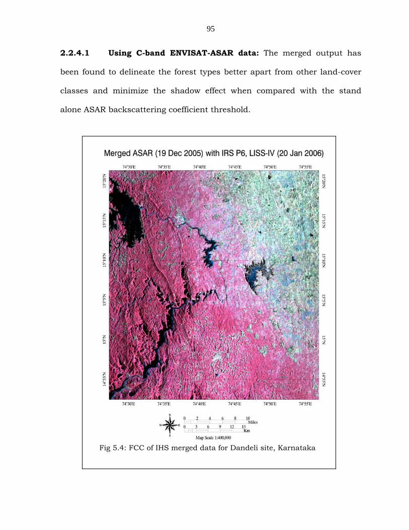
Fig 5.9 (i) shows the intensity image in HH polarization for which different

textural measures was computed. FCC generated from homogeneity, mean

and entropy (fig 5.9(ii)) has enabled better discrimination as compared to

the others. Texture measures generated from GLCM increased the ability to

discriminate different land cover classes using single date and single

polarized data. Different land cover classes showed different textural

measures. Forests exhibit a wide variety of texture influenced by SAR

parameters and forest characteristics.

Fig 5.9: i) 29 Oct 07 HH Image ii) FCC of Homogeneity, Mean and Entropy in parts of Bilaspur, Chattisgarh

i ii

The FCC (fig 5.9 (ii)) showed a good seperability between agriculture and

forest regions as well as dense and open forests. Combinations of various

Fig 5.9: i) ASAR HH image of 29th Oct07 ii) FCC of homogeneity (Red), Mean (Green) and Entropy (Blue) in Achanakmar-Amarkantak biosphere Reserve

109

textural measures showed improvement over single-set texture measure

because of their different, complementary information.

The FCC generated from homogeneity, mean and entropy was analyzed

using maximum likelihood algorithm. The thematic map thus generated, is

shown as fig 5.10.

Homogeneity values were high; forests and agriculture had high

homogeneity values than other classes. There was no change of

homogeneity values (ranged between 0.1 and 0.2) between agriculture and

forested regions.

Entropy values in the study area ranged between 1 and 3. Entropy values

were high (ranged between 2.5 and 4) for the scrub and hilly terrain areas.

Entropy, which is a measure of the degree of disorder, is larger when the

image is texturally non-uniform or heterogeneous. Entropy band helped

discrimination of open and dense forests within the forested area. The

values of the entropy increased with decreasing density viz., dense forests

showed low entropy values than open forests. The mean backscatter band

showed the discrimination between the agriculture and forested areas.

Areas of slope facing the sensor in the terrain areas have been misclassified

as scrub regions. Backward slope is mostly under the shadow and is

misclassified as water.

110

Accuracy assessment of the classified map generated from ASAR data was

carried out using ground truth points and IRS P6 LISS-III data. Error matrix

and kappa statistics were generated and given in Table 5.5.

Fig 5.10: Vegetation classified map of Achanakmar-Amarkantak Biosphere Reserve using texture measures

81◦40’00”81◦30’00”81◦20’00”

22◦ 2

0’00

”22

◦ 30’

00”

22◦ 4

0’00

”

22◦20’00”

22◦30’00”

22◦40’00”

±

111

The over all classification accuracy and kappa statistics were 79.14% and

0.74, respectively. The discrimination of forests was quite good with the use

of the texture measures. However, there was some misclassification of

forests as barren areas in the hilly terrain regions. In some parts, croplands

and barren lands have been misclassified as current fallows. An overall

classification accuracy of 79% was achieved.

Table 5.5: Accuracy table and Kappa statistics of classified map generated from texture measures

Class Producer's accuracy User's accuracy Kappa statistics Dense forest 84.67% 76.47% 0.723 Open forest 94.12% 80.00% 0.759 Barren 60.00% 81.82% 0.786 Current fallow 83.33% 62.50% 0.573 Scrub 70.37% 90.48% 0.869 Agriculture 85.71% 80.00% 0.767

Texture measures using GLCM were generated from ALOS-PALSAR data

and the classified map generated gave the same result as the classified map

generated from backscattering coefficient of L-band PALSAR data. No

additional information was obtained from texture measures.

As the classified map generated from ASAR data was not able to

discriminate agriculture and forests, computation of texture measures was

carried out. The results suggest the possible use and scope of single date

and single polarized C band SAR backscatter and SAR-derived texture

measures for vegetation type classification.

112

5.3 CONCLUSIONS:

In the present study, three techniques for vegetation classification were

carried out. These techniques successfully discriminated land cover classes

viz., agriculture, barren, moist deciduous forests, teak mixed forests (multi-

sensor fusion); open forests, dense forests, scrub (using texture measures);

teak plantations (using first order statistics). Based on the observations and

experience in three study areas, we can say that these methods are not

universal in nature. The classification accuracy depends on many factors

viz., behavior of target with the sensor, season of the acquisition, contrast of

backscatter among different land cover classes.

The vegetation classification can be still enhanced with the use of

interferometric spaceborne SAR data and polarimetric airborne SAR data

techniques which are discussed in next chapters.