Chapter 6 Arbitrage Relationships for Call and Put Options · Chapter 6 Arbitrage Relationships for Call and Put Options ... Throughout this chapter we shall adopt the following notation

Chapter 6Arbitrage Relationships for Call and Put Options

Recall that a risk-free arbitrage opportunity arises when an investment is identified thatrequires no initial outlays yet guarantees nonnegative payoffs in the future. Such oppor-tunities do not last long, as astute investors soon alter the demand and supply factors,causing prices to adjust so that these opportunities are closed off. In this chapter we shalluse simple arbitrage arguments to obtain some basic boundary conditions for call and putoptions. The beauty of the pricing relationships derives from the fact that they requireno assumptions on the statistical process driving security prices. Also, no severe assump-tions are made concerning the risk behavior of investors. The simple requirement is thatinvestors like more money than less. This chapter also investigates conditions under whichit is more appropriate to exercise options than to sell them. The final section explores somefundamental pricing relationships that exist between put and call options.

The primary objectives of this chapter are the following:

• To derive boundary prices for call and put option prices from arbitrage arguments;

• To explain when exercising options is not appropriate;

• To understand how mispriced options can be traded to lock in arbitrage free profits;and

• To describe pricing relationships between put and call options.

Throughout this chapter we shall adopt the following notation. The current time ist = 0. The option expires at date T , where T is expressed in years. The time to thejthex-dividend date is tj, and the size of dividend declared at ex-dividend date tj is dj . Weare interested only in ex-dividend dates prior to expiration. In most cases, the number ofdates in the interval is less than three. Throughout this chapter we assume the risk freerate, r, is constant. Let B(s, t) be the price at time s of a riskless pure discount bond thatpays out $1 at time t. Then

B(s, t) = e−r(t−s) ≤ 1

and with s = 0:B(0, t) = e−rt

Chapter 6 : Arbitrage Relationships. Copyright c©by Peter Ritchken 1999 2

Clearly, discount bond prices decrease with maturity. That is, for t > s

B(0, t) < B(0, s) < 1

If 1 dollar is invested in the risk free asset (bank) at time s, this amount of money willgrow continuously at rate r, and at time t the value will be 1er(t−s). Let G(s, t) = er(t−s)

represent the account value. Clearly, G(s, t) = 1/B(s, t).

Finally, as discussed in chapter 4, a call option that can only be exercised at the expi-ration date (and not before) is called a European option. An American option must havea value at least as great as a European option, since the former has all the properties ofthe latter plus the additional early exercise feature. This characteristic is used in derivingseveral properties in this chapter.

Riskless Arbitrage and the Law of One Price

This chapter frequently uses the argument that there are no riskless arbitrage opportu-nities. Below we provide some illustrative examples.

Example

(i) Consider the following investment opportunities:

• For $70, an investor can buy (sell) a share of A, which, at the end of the period, willeither appreciate to $120 or depreciate to $60, depending on whether the economy”booms” or not.

• For $b, an investor can buy (sell) a share of B that will either appreciate to $100 ordepreciate to $50, depending on the same economic factors.

• A riskless investment where each dollar grows to $1.10.

✟✟✟✟✟✟✟

❍❍❍❍❍❍❍

$70

$120

$60

✟✟✟✟✟✟✟

❍❍❍❍❍❍❍

$b

$100

$50

✟✟✟✟✟✟✟

❍❍❍❍❍❍❍

$1

$1.10

$1.10

Security A Security B Riskless Security

What is the maximum price b can take?


✟✟✟✟✟✟✟

❍❍❍❍❍❍❍

$(70-b)

120-100 = $20

60 - 50 = $10

To answer this question, first consider a portfolio consisting of one share of A and a shortposition of one share in B. The payouts of this portfolio are shown below:

Clearly, all investors would prefer the final dollar payout of this portfolio to a certain payoutof $10. To avoid a possible “free lunch”, the present value of this portfolio must exceed thepresent value of $10. That is, (70 − b) > 10/1.10 = $9.09, or b < $60.91. If, for example,b = $64, then a “free lunch” would exist. Specifically, an investor could establish a zeroinitial investment position by selling one share of B for $64, borrowing $6, and using thetotal proceeds to purchase one share of A. The $6 debt will grow to 6× 1.1 = $6.60 in oneyear. The final payouts of this strategy are shown below:

✟✟✟✟✟✟✟

❍❍❍❍❍❍❍

$0

120 - 100 - 6.6 = $13.40

60 - 50 - 6.6 = $3.40

To avoid this free lunch, the price of a share of B must satisfy b < $60.91.

Assume a third investment, C, provided the following payout:

✟✟✟✟✟✟✟

❍❍❍❍❍❍❍

$c

$120

$60

To avoid riskless arbitrage, c must equal $70. To see this, note that this investment hasidentical payouts to A. If C exceeded $70, investors would buy A and sell C to lock into


profits. Conversely, if C was lower than $70, investors would buy C and sell A to lock intoprofits.

The law of one price states that if two securities produce identical payouts in all futurestates, then, to avoid riskless arbitrage, their current prices must be the same. We shall usethis law frequently in this and later chapters.

Call Pricing Relationships

In this section we establish bounds on call options and we investigate conditions underwhich it may be optimal to exercise the call option. Our first property provides a boundfor the price of a call option when the underlying stock pays no dividends over the lifetimeof the option.

Property 1

If there are no dividends prior to expiration, then to prevent arbitrage op-portunities, the call price should never fall below the maximum of zero orthe stock price minus the present value of the strike. That is,

C0 ≥ Max[0, S0 − XB(0, T )]

Proof: Consider two portfolios, A and B. A contains one European call option and Xpure discount bonds with a face value of $1 each and maturity T. B contains a long positionin the stock.

Exhibit 1 llustrates the prices of the two portfolios at the expiration date of the option.Note that the future value of portfolio A is never lower than the future value of portfolio B.

Exhibit 1: Bounding Call Prices

Portfolio Current Value ST < X ST ≥ X

A C0 +XB(0, T ) 0 + X (ST − X) + XB S0 ST ST

VA(T ) > VB(T ) VA(T ) = VB(T )

If an investor bought portfolio A and sold portfolio B, then, at the expiration date, thecombined portfolio, P , would have value Vp(T ), given by Vp(T ) = VA(T ) − VB(T ), whereVA(T ) and VB(T ) define the values of the portfolios A and B at time T.


If the call option expired in the money, then VA(T ) = VB(T ) and, hence, Vp(T ) = 0.However, if the call expired worthless, then, Vp(T ) = VA(T ) − VB(T ) ≥ 0. The portfolio,P , thus, can never lose money and has a chance of making money. Let us now consider theinitial cost of the portfolio, Vp(0). Since this portfolio has a nonnegative terminal value, itmust be worth a nonnegative amount now. Hence

Vp(0) = VA(0) − VB(0) ≥ 0

Equivalently, VA(0) ≥ VB(0). Substituting for VA(0) and VB(0), leads to

C0 ≥ S0 − XB(0, T )

Since a European call option must have value no less than S0−XB(0, T ), so must an Amer-ican option. Of course, since call options offer the holder the right to purchase securities ata particular price, this right must have some value. Hence, C0 ≥ 0. The result then follows.

Example

Consider a stock currently priced at $55, with a three-month $50 strike price call available.Assume no dividends occur prior to expiration, and the riskless rate, r, is 12%. The lowerbound on the price is given by the following:

C0 ≥ Max[0, S0 − XB(0, T )] = Max[0, 55 − 50e−0.12(3/12) ] = $6.48

We now establish bounds on the call price when the underlying security pays a dividend.

Property 2

If a stock pays a single dividend of size d1 at time t1, then to prevent risklessarbitrage, the call price should never fall below

Max[C1, C2]

where

C1 = Max[0, S0 − XB(0, t1)]C2 = Max[0, S0 − d1B(0, t1)− XB(0, T )]

Proof: C1, and C2 correspond to values from specific trading strategies.


Strategy 1: Exercise the Call Option Just Prior to Ex-Dividend Date

Assume the option is exercised just prior to the ex-dividend date. Then, by using thesame argument used to prove Property 1, we see that the call price must exceed the stockprice less the present value of the strike.

Strategy 2: Exercise the Call Option at Expiration

If the dividend is sacrificed and the option held to expiration, the call value must exceedC2. To prove this result, consider two portfolios, A and B. A contains d1 bonds that payout $d1 at time t1 and X bonds that pay out X dollars at time T. In addition, a call optionis held. All dividends received at time t1 are invested in the risk-free asset. Portfolio Bcontains a long position in the stock. Exhibit 2 illustrates the payoffs that occur if thestrategy of exercising the call at the expiration date is followed.

Exhibit 2: Bounding Call Prices with Dividends

Portfolio Current Value ST < X ST ≥ X

A C0 + XB(0, T ) + d1B(0, t1) X + d1G(t1, T ) ST + d1G(t1, T )B S0 ST + d1G(t1, T ) ST + d1G(t1, T )

VA(T ) ≥ VB(T ) VA(T ) = VB(T )

Note that in portfolio A, the d1 dollars received at time t1 are reinvested in the risklesssecurity and thus grow to d1G(t1, T ) at expiration.

Since VA(T ) ≥ VB(T ), it must follow that,to prevent arbitrage opportunities, VA(0) ≥VB(0). Hence, C0 ≥ C2.

Since at the current time the optimal strategy is unknown, the actual call value shouldexceed the payoffs obtained under these two strategies. Hence, C0 ≥ Max(C1, C2). Thiscompletes the proof.

Example

Reconsider the previous problem, but now assume a dividend of $5 is paid after one month.The lower bound on the call price is given by Max(C1, C2), where

C1 = Max[0, S0 − Xe−rt1 ] = Max(0, 55 − 49.5) = $5.50,C2 = Max[0, S0 − d1e

−rt1 − Xe−rT ] = Max(0, 55 − 4.95 − 48.52) = $1.53.

Hence, C0 ≥ $5.50. Note that the effect of dividends has been to lower the lower boundof the call option.


Example

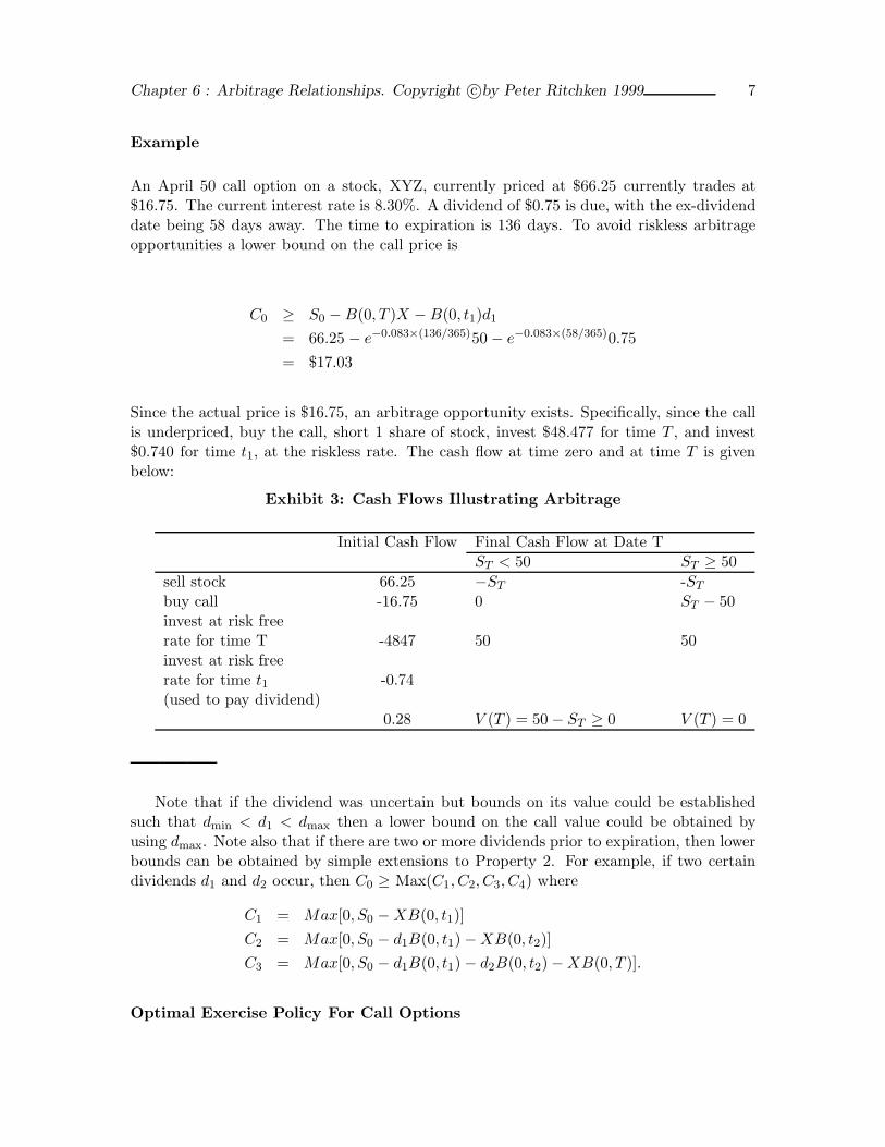
An April 50 call option on a stock, XYZ, currently priced at $66.25 currently trades at$16.75. The current interest rate is 8.30%. A dividend of $0.75 is due, with the ex-dividenddate being 58 days away. The time to expiration is 136 days. To avoid riskless arbitrageopportunities a lower bound on the call price is

C0 ≥ S0 − B(0, T )X − B(0, t1)d1

= 66.25 − e−0.083×(136/365)50 − e−0.083×(58/365)0.75= $17.03

Since the actual price is $16.75, an arbitrage opportunity exists. Specifically, since the callis underpriced, buy the call, short 1 share of stock, invest $48.477 for time T , and invest$0.740 for time t1, at the riskless rate. The cash flow at time zero and at time T is givenbelow:

Exhibit 3: Cash Flows Illustrating Arbitrage

Initial Cash Flow Final Cash Flow at Date TST < 50 ST ≥ 50

sell stock 66.25 −ST -ST

buy call -16.75 0 ST − 50invest at risk freerate for time T -4847 50 50invest at risk freerate for time t1 -0.74(used to pay dividend)

0.28 V (T ) = 50− ST ≥ 0 V (T ) = 0

Note that if the dividend was uncertain but bounds on its value could be establishedsuch that dmin < d1 < dmax then a lower bound on the call value could be obtained byusing dmax. Note also that if there are two or more dividends prior to expiration, then lowerbounds can be obtained by simple extensions to Property 2. For example, if two certaindividends d1 and d2 occur, then C0 ≥ Max(C1, C2, C3, C4) where

C1 = Max[0, S0 − XB(0, t1)]C2 = Max[0, S0 − d1B(0, t1)− XB(0, t2)]C3 = Max[0, S0 − d1B(0, t1)− d2B(0, t2)− XB(0, T )].

Optimal Exercise Policy For Call Options


The previous property established bounds on the call prices by considering the effectof specific exercise strategies: namely, exercising immediately, just prior to an ex- dividenddate, or at expiration. However, other exercising times are possible. In this section we showthat if exercising is ever appropriate for call options, it should be done at expiration orimmediately prior to an ex-dividend date.

Property 3

(i) The early exercise of a call option on a stock that pays no dividends priorto expiration is never optimal.(ii) For such a stock, the price of an American call option equals the priceof an otherwise identical European call.

Proof: To prove this result we must show that for a stock that pays no dividends over thelifetime of the option, the value of a call option unexercised is always equal to or greaterthan the value of the option exercised.

Let tp be any time point prior to expiration. From Property 1, the lower bound on thecall price at time tp is the stock price, S(tp), less the present value of the strike, XB(tp, T ).Hence, C(tp) ≥ Max[0, S(tp) − XB(tp, T )]. Note that the right hand side of the equationexceeds the intrinsic value of the option, S(tp) - X. Hence, early exercise is not optimal.

From Property 3 we see that early exercise of an American call option on a stock thatpays no dividends over the lifetime of the option is never appropriate. Therefore, the valueof the right to exercise the option prior to expiration must be zero. Thus, an American calloption must have the same value as a European call.

Property 4

If a stock pays dividends over the lifetime of the option, then the Americancall option may be worth more than a European call option.

Proof: To prove this result, we shall show that just prior to an ex-dividend date theremay be an incentive to exercise early. To see this, consider an extreme case in which afirm pays all its assets as cash dividends. Clearly, any in-the-money call options shouldbe exercised prior to the ex-dividend date, since after the date the call value will be zero.Note that if the option was European, its value before the ex-dividend date would be zero,whereas the American option would have positive value.


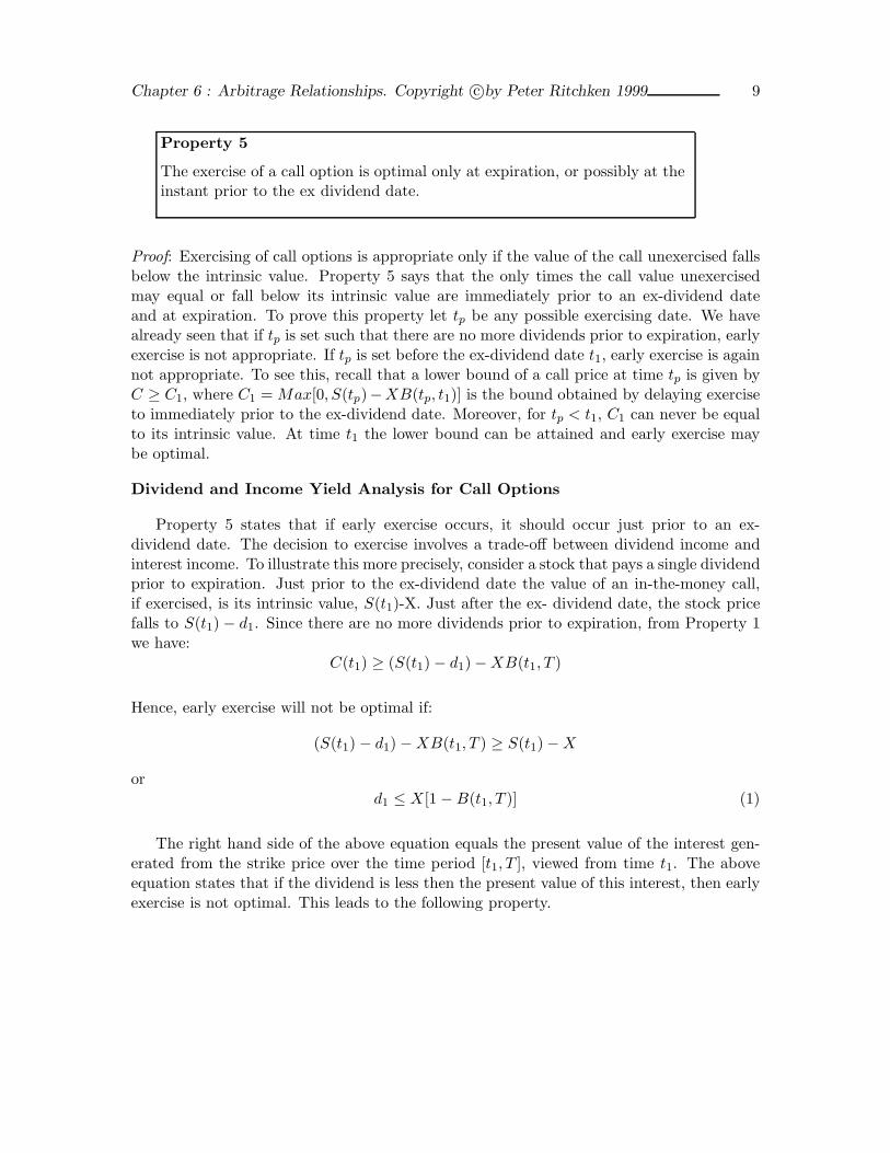
Property 5

The exercise of a call option is optimal only at expiration, or possibly at theinstant prior to the ex dividend date.

Proof: Exercising of call options is appropriate only if the value of the call unexercised fallsbelow the intrinsic value. Property 5 says that the only times the call value unexercisedmay equal or fall below its intrinsic value are immediately prior to an ex-dividend dateand at expiration. To prove this property let tp be any possible exercising date. We havealready seen that if tp is set such that there are no more dividends prior to expiration, earlyexercise is not appropriate. If tp is set before the ex-dividend date t1, early exercise is againnot appropriate. To see this, recall that a lower bound of a call price at time tp is given byC ≥ C1, where C1 = Max[0, S(tp)−XB(tp, t1)] is the bound obtained by delaying exerciseto immediately prior to the ex-dividend date. Moreover, for tp < t1, C1 can never be equalto its intrinsic value. At time t1 the lower bound can be attained and early exercise maybe optimal.

Dividend and Income Yield Analysis for Call Options

Property 5 states that if early exercise occurs, it should occur just prior to an ex-dividend date. The decision to exercise involves a trade-off between dividend income andinterest income. To illustrate this more precisely, consider a stock that pays a single dividendprior to expiration. Just prior to the ex-dividend date the value of an in-the-money call,if exercised, is its intrinsic value, S(t1)-X. Just after the ex- dividend date, the stock pricefalls to S(t1)− d1. Since there are no more dividends prior to expiration, from Property 1we have:

C(t1) ≥ (S(t1)− d1)− XB(t1, T )

Hence, early exercise will not be optimal if:

(S(t1)− d1)− XB(t1, T ) ≥ S(t1)− X

ord1 ≤ X[1− B(t1, T )] (1)

The right hand side of the above equation equals the present value of the interest gen-erated from the strike price over the time period [t1, T ], viewed from time t1. The aboveequation states that if the dividend is less then the present value of this interest, then earlyexercise is not optimal. This leads to the following property.


Property 6

(i) Early exercise of the American call option on a stock that pays a singledividend prior to expiration is never optimal if the size of the dividend is lessthan the present value of interest earned on the strike from the ex dividenddate to expiration.

(ii) Early exercise of an American call option on a stock that pays multipledividends prior to expiration is never optimal if at each ex dividend date, thepresent value of all future dividends till expiration is less than the presentvalue of interest earned on the strike, from the ex dividend date to expiration.

Example

A stock is priced at $55. It pays a $5.00 in one month. Interest rates are 12% per year. Athree month call option with strike $50 has a lower bound given by:

C0 ≥ Max(C1, C2)= Max(5.50, 1.53) = $5.50.

Early exercise of this option will not be appropriate if the size of the dividend (d1 = $5)is lower than the foregone interest, f , which is given by:

f = X[1− e−r(T−t1 ] = 50[1 − e−0.12×(2/12)] = $0.99.

Since d1 > f , exercise just prior to the ex dividend date may be appropriate.

Note if there are no dividends, d1 is zero, the early exercise condition in equation (1) issatisfied and premature exercising is not optimal. Moreover, from equation (1), the optionshould not be exercised if the strike price exceeds the value X∗ where

X∗ = d1/[1− B(t1, T )].

If equation (1) is satisfied, early exercise of the option is never optimal. If the equationis not satisfied, then early exercise may be optimal. Of course, the benefit from exercisingis that the intrinsic value is received prior to the stock price dropping by the size of thedividend. This benefit is partially offset by the loss of the time premium of the option. Ifat the ex- dividend date the stock price is sufficiently high, then the time premium is verysmall, and if equation (1) does not hold, early exercise is quite likely. We defer further detailsof this point to Chapter 9, where explicit models for the time premium are established,andrules are established for precise timing of exercise.


Put Pricing Relationships

In this section some arbitrage restrictions for American put options are derived. UnlikeAmerican call options, early exercise of American put options may be optimal even if theunderlying stock pays no dividends. Before considering early exercise policies, we firstestablish some pricing bounds. As with Property 2 for calls, we obtain pricing bounds byconsidering specific exercise strategies for put options.

Property 7

Consider a stock that pays a single dividend of size d1 at time t1. AnAmerican put option must satisfy the following:

P0 ≥ Max[P1, P2]

where

P1 = Max[0,X − S0]P2 = Max[0, (X + d1)B(0, t1)− S0]

Proof. To obtain these bounds we consider two strategies. The first is to exercise immedi-ately; the second strategy is to exercise just after the ex dividend date. Other strategies,such as exercising just before the ex-dividend date, or exercising at expiration, lead toweaker bounds.

Strategy 1: Exercise Immediately

Since a put option gives the holder the right (but not the obligation) to sell stock at thestrike price, the put option must have nonnegative value. Further, if exercised immediately,its intrinsic value is obtained with the loss of a possible time premium. Hence, P0 ≥ P1.

Strategy 2: Exercise Immediately After the Ex-dividend Date Now consider thestrategy of exercising the put option just after the ex-dividend date, t1. Then P0 ≥ P2. Tosee this, consider two portfolios, A and B, where A consists of the put and B consists of ashort position in the stock together with (X + d1) bonds that mature at time t1. Exhibit 4shows their values at time t1, given that the put is exercised.

Exhibit 4: Bounding Put Options

Portfolio Current Value Value at date t1S(t1) < X S(t1 ≥ X

A P0 X − S(t1 0B (d1 + X)B(0, t1)− S0 X − S(t1) 0

VA(T ) = VB(T ) VA(T ) > VB(T )


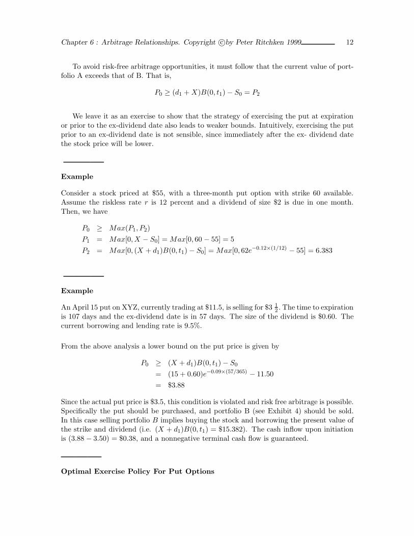
To avoid risk-free arbitrage opportunities, it must follow that the current value of port-folio A exceeds that of B. That is,

P0 ≥ (d1 + X)B(0, t1)− S0 = P2

We leave it as an exercise to show that the strategy of exercising the put at expirationor prior to the ex-dividend date also leads to weaker bounds. Intuitively, exercising the putprior to an ex-dividend date is not sensible, since immediately after the ex- dividend datethe stock price will be lower.

Example

Consider a stock priced at $55, with a three-month put option with strike 60 available.Assume the riskless rate r is 12 percent and a dividend of size $2 is due in one month.Then, we have

P0 ≥ Max(P1, P2)P1 = Max[0,X − S0] = Max[0, 60 − 55] = 5P2 = Max[0, (X + d1)B(0, t1)− S0] = Max[0, 62e−0.12×(1/12) − 55] = 6.383

Example

An April 15 put on XYZ, currently trading at $11.5, is selling for $3 12 . The time to expiration

is 107 days and the ex-dividend date is in 57 days. The size of the dividend is $0.60. Thecurrent borrowing and lending rate is 9.5%.

From the above analysis a lower bound on the put price is given by

P0 ≥ (X + d1)B(0, t1)− S0

= (15 + 0.60)e−0.09×(57/365) − 11.50= $3.88

Since the actual put price is $3.5, this condition is violated and risk free arbitrage is possible.Specifically the put should be purchased, and portfolio B (see Exhibit 4) should be sold.In this case selling portfolio B implies buying the stock and borrowing the present value ofthe strike and dividend (i.e. (X + d1)B(0, t1) = $15.382). The cash inflow upon initiationis (3.88 − 3.50) = $0.38, and a nonnegative terminal cash flow is guaranteed.

Optimal Exercise Policy For Put Options


Unlike call options, it may be optimal to exercise put options prior to expiration. To seethis, consider a stock whose value falls to zero. In this case the put holder should exercisethe option immediately. This follows, since if the investor delays action, the interest receivedfrom the strike price is lost. This leads to property 8

Property 8

Early exercise of in the money put options may be optimal.

Immediately after an ex-dividend date, the holder of an in-the-money put option whoalso owns the stock may exercise the option. This is especially likely if the put is deep inthe money and no more dividends are to be paid prior to expiration. By not exercisingthe option, the holder foregoes the interest that could be obtained from investing the strikeprice. Just prior to an ex-dividend date, early exercise of a put option is never optimal.Since dividends cause the stock price to drop further, investors will always prefer delayingexercising to just after the ex- dividend date.

Since early exercise of American put options is a real possibility, these contracts will bemore valuable than their European counterparts. Moreover, because American put optionscan be more valuable exercised than not exercised, it must follow that on occasion Europeanput options could have values less than their intrinsic values. In other words, it is possible forEuropean put options to command a negative time premium. This fact will be reconsideredlater.

Property 9

Immediate exercise of a put on a dividend paying stock is not optimal ifthe size of the dividend exceeds the interest income on the strike from thecurrent date to the ex-dividend date.

Proof: Recall that in the absence of dividend payments, early exercise of a put may beoptimal because interest income can be earned on the proceeds obtained as soon as theoption is exercised. Deferring exercise implies interest income is being foregone. For adividend paying stock, delaying exercise also results in foregoing interest income. However,by exercising early the investor does not profit from the discrete downward jump in thestock price that occurs at the ex-dividend date. If the interest earned on the strike fromnow until the ex-dividend date is smaller than the size of the dividend, then clearly it isbeneficial to wait.

For a dividend paying stock, we can obtain a bound on the put price by considering thestrategy of delaying exercise until just after the ex-dividend date. Specifically, viewed fromtime t, t < t1, we have, from Property 7:

P (t) ≥ (X + d1)B(t, t1)− S(t1)


Clearly immediate exercise at time t is not optimal if

X − S(t) ≤ (X + d1)B(t, t1)− S(t1)

which upon simplification reduces to

d1B(t, t1) ≥ X[1− B(t, t1)]d1 ≥ X[er(t1−t) − 1]

The right hand side of this equation represents the interest income generated by thestrike price from date t to t1. Note that as t tends to t1, the right hand side of this equationtends to zero and the condition will eventually be satisfied. Let t∗ be chosen such that

d1 = X[er(t1−t∗) − 1].

Then, over the interval [t∗, t1] early exercise of an American put will never be optimal.

If the current time t, falls in the interval [t∗, t1], then early exercise, prior to t1, is notoptimal. If the current time t falls outside this interval i.e. if t < t∗, then early exercise maybe optimal. Indeed if the stock price is sufficiently low, or if interest rates are sufficientlyhigh, then early exercise is a distinct possibility.

The above result generalizes to the case where multiple dividends occur prior to expi-ration. In this case the interval [t∗, t1] will be wider than the interval obtained by ignoringall but the first ex-dividend date, because the effect of the additional dividends providesincreased incentives to delaying exercise.

A direct implication of this property is that the probability of exercise decreases as thesize of the dividend increases.

Strike Price Relationships For Call and Put Options

The next property provides the relationships between options with different strike prices.

Property 10

Let C1, C2, C3 (P1, P2, P3) represent the cost of three call (put) options thatare identical in all aspects except strike prices. Let X1 ≤ X2 ≤ X3 bethe three strike prices, and for simplicity, let X3 −X2 = X2 −X1. Then, toprevent riskless arbitrage strategies from being established, the option pricesmust satisfy the following conditions:

C2 ≤ (C1 + C3)/2P2 ≤ (P1 + P3)/2


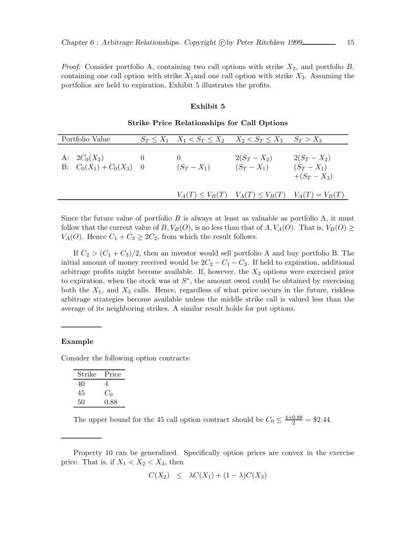
Proof: Consider portfolio A, containing two call options with strike X2, and portfolio B,containing one call option with strike X1and one call option with strike X3. Assuming theportfolios are held to expiration, Exhibit 5 illustrates the profits.

Exhibit 5

Strike Price Relationships for Call Options

Portfolio Value ST ≤ X1 X1 < ST ≤ X2 X2 < ST ≤ X3 ST > X3

A: 2C0(X2) 0 0 2(ST − X2) 2(ST − X2)B: C0(X1) +C0(X3) 0 (ST − X1) (ST − X1) (ST − X1)

+(ST − X3)

VA(T ) ≤ VB(T ) VA(T ) ≤ VB(T ) VA(T ) = VB(T )

Since the future value of portfolio B is always at least as valuable as portfolio A, it mustfollow that the current value of B,VB(O), is no less than that of A,VA(O). That is, VB(O) ≥VA(O). Hence C1 + C3 ≥ 2C2, from which the result follows.

If C2 > (C1 + C3)/2, then an investor would sell portfolio A and buy portfolio B. Theinitial amount of money received would be 2C2 −C1 −C3. If held to expiration, additionalarbitrage profits might become available. If, however, the X2 options were exercised priorto expiration, when the stock was at S∗, the amount owed could be obtained by exercisingboth the X1, and X3 calls. Hence, regardless of what price occurs in the future, risklessarbitrage strategies become available unless the middle strike call is valued less than theaverage of its neighboring strikes. A similar result holds for put options.

Example

Consider the following option contracts:

Strike Price40 445 C0

50 0.88

The upper bound for the 45 call option contract should be C0 ≤ 4+0.882 = $2.44.

Property 10 can be generalized. Specifically option prices are convex in the exerciseprice. That is, if X1 < X2 < X3, then

C(X2) ≤ λC(X1) + (1− λ)C(X3)


P (X2) ≤ λP (X1) + (1− λ)P (X3)

where λ = (X3 − X2)/(X3 − X1).

Put-Call Parity Relationships

In this section we shall develop pricing relationships between put and call options.

European Put-Call Parity: No Dividends

Property 11

With no dividends prior to expiration, a European put should be priced as aEuropean call plus the present value of the strike price less the stock price.That is:

PE0 = CE

0 + XB(0, T )− S0

where the superscript E emphasizes the fact that the options are European.

Proof: Under the assumption of no dividends and no premature exercising consider port-folios A and B, where A consists of the stock and European put and B consists of theEuropean call with X pure discount bonds of face value $1 that mature at the expirationdate. Exhibit 6 compares their future values.

Exhibit 6 : Put-Call Parity

Portfolio Current Value Value at date TST < X ST ≥ X

A P0 + S0 X ST

B C0 + XB(0, T ) X ST

VA(T ) = VB(T ) VA(T ) = VB(T )

To avoid riskless arbitrage opportunities, it must follow that the current value of the twoportfolios are the same. This leads to the result. This relationship is called the Europeanput-call parity equation.

Example

Given the price of a stock is $55, the price of a three-month 60 call is $2, and the risklessrate is 12 percent, then the lower bound for a three- month 60 put option can be derived.


Specifically,

P0 = C0 + XB(0, T ) − S0

= 2 + 60e−0.12×(3/12) − 55= $5.23

European Put-Call Parity Equations with Dividends

Property 12

Consider a stock that pays a single dividend of size d1 at time t1 < T . AnEuropean put option is priced as follows:

PE0 = CE

0 + XB(0, T ) + d1B(0, t1)− S0

Proof: Consider a stock that pays a dividend d1, at time t1. Consider the following twoportfolios, A and B. Portfolio A contains the stock and put option. Portfolio B contains thecall and X pure discount bonds of face value $1 that mature at the expiration date, alongwith d1, pure discount bonds that mature at time t1. Exhibit 7 illustrates the terminalvalues under the assumption that all dividends or payouts are reinvested at the risklessrate.

Exhibit 7

Arbitrage Portfolio-Put-Call Parity with Dividends

Portfolio Current Value Value at date TST < X ST ≥ X

A P0 + S0 X + d1G(t1, T ) ST + d1G(t1, T )B C0 + XB(0, T ) + d1B(0, t1) X + d1G(t1, T ) ST + d1G(t1, T )

VA(T ) = VB(T ) VA(T ) = VB(T )

Since the terminal values of the two portfolios are the same regardless of the future stockprice, it must follow that, to avoid riskless arbitrage opportunities, the current portfoliovalues must be the same. This then leads to the result.

The put-call parity equation not only values a European put option in terms of stocks,calls, and bonds, but also provides a mechanism for replicating a put option. That is, aportfolio containing one call option, X pure discount bonds maturing at time T, d1 pure


discount bonds maturing at time t1, and a short position in the stock completely replicatesthe payouts of a put option.

Indirect Purchasing of Puts: A Synthetic Put

From put-call parity:P0 = C0 + XB(0, T ) − S0.

Hence a portfolio consisting of a European call option together with X pure discountbonds and a short position in the stock produces the same payout as an European put.This portfolio is called a synthetic put.

Indirect Purchasing of Stock: A Synthetic Stock

From put-call parity:S0 = XB(0, T ) + C0 − P0.

Hence, rather than buy the stock directly, one can buy it ”indirectly” by purchasing Xdiscount bonds maturing at time T , by buying a call option, and by selling a European put.

Indirect Purchasing of Calls: A Synthetic Call

Since P0 = C0 + XB(0, T )− S0, we have

C0 = S0 + P0 − XB(0, T )

Thus, a call option can be replicated by buying the stock and put option and borrowingthe present value of the strike.

American Put-Call Parity Relationships: No Dividends

Property 13

With no dividends prior to expiration, the value of an American put optionis related to the American call price by

P0 ≥ C0 + XB(0, T ) − S0

Proof: Property 13 follows directly from Property 9 and the recognition that American putsare more valuable than European options (that is, P0 ≥ PE

0 ). Note that since CE0 = C0 ≥ 0,

we have PE0 ≥ C0 + XB(0, T ) − S0. That is, a European put should always be priced no

lower than the present value of the strike price less the stock price. Note that this lowerbound is less than the intrinsic value, X − S0. European put options could have negativetime premiums.


Property 14

With no dividends prior to expiration, the value of an American put optionis restricted by:

P0 ≤ C0 − S0 +X

Proof: Consider portfolio A, which contains a call and X dollars invested in the risklessasset, and portfolio B, which contains a put option together with the stock. Exhibit 8 showsthe cash flows of the two portfolios. Since the value of portfolio B depends on whether theput was exercised prematurely, both cases must be considered.

Exhibit 8Bounding American Put Option Prices

Portfolio Value Value at date t Value at date T( if the put is exercised) ST < X ST ≥ X

A: C0 + X Ct + XG(0, t) XG(0, T ) (ST − X) + XG(0, T )B: P0 + S0 X X ST

VA(T ) > VB(T ) VA(T ) > VB(T ) VA(T ) > VB(T )

If the put is exercised early, the stock is delivered in receipt for $X. Note that, in thiscase, the value of the bonds alone in portfolio A exceeds the value of portfolio B. If the putis held to expiration, then portfolio A will be more valuable than portfolio B, regardless ofthe future stock price. Clearly, to avoid risk-free arbitrage opportunities, the current valueof portfolio A must be no smaller than the value of portfolio B. Hence, C0 + X ≥ P0 + S0,from which the result follows.

Example

The stock trades at $60, a three month at the money call trades at $2, and the risklessrate is 12 percent. Then, the at the money put is constrained by: PA

0 ≤ C0 + X − S0 =2 + 60− 55 = 7, and PA

0 ≥ C0 + XB(0, T ) − S0 = 5.23. Hence, 5.23 ≤ PA0 ≤ 7.

Other Pricing Relationship Properties

In this section we state several additional properties. The proofs are left as exercises.


Property 15

(i) The difference between the prices of two otherwise identical Europeancalls (puts) cannot exceed the present value of the difference between theirstrike prices.

CE(X1)− CE(X2) ≤ (X2 − X1)B(0, T )PE(X2)− PE(X1) ≤ (X2 − X1)B(0, T )

(ii) The difference between the prices of two otherwise identical Americancalls (puts) cannot exceed the difference between their strike prices.

C(X1)− C(X2) ≤ (X2 − X1)P (X2)− P (X1) ≤ (X2 − X1)

where X2 ≥ X1.

Property 16

(i) The difference in prices between two American calls and two Americanputs is bounded below as follows:

[C(X1)− C(X2)]− [P (X1)− P (X2)] ≥ (X2 − X1)B(0, T )

where X2 ≥ X1. This relationship is called the box spread lower boundarycondition.

Property 17

Option prices are homogeneous of degree one in the stock price and strikeprice. That is:

C(λS, λX, T ) = λC(S,X, T )P (λS, λX, T ) = λP (S,X, T )

The property is rather obvious for the case when the numeraire is just rescaled. Forexample, if the stock is measured in cents rather than dollars, then, as long as the strike ismeasured in cents as well, the option price remains correctly priced in the new numeraire ofcents. Property 17 implies that when a stock splits, the strike price can be adjusted withoutcreating problems.

Example


Assume a stock is priced at $110. Acall trades with strike $100. If the stock splits intotwo shares of $55 each, then the terms of the option contract has to be modified. From thisproperty, an appropriate adjustment would be to exchange the original call option with twooptions each controlling one new share at a strike price of $50 per share. The value of thesetwo options would equal the value of the original single contract.

One has to be careful in applying this property in certain cases. For example, if thestock returns process is not independent of the level of the stock price, then the propertyis not valid. As an extreme example, consider a firm that had stock priced at $100 and anoption with strike $120. Now assume the firm changes its strategy from a risky to a risklessone in such a way that the new stock price, is $50. Say the new strike is set at $60. Withriskless rates equal to 5% per year, there is no chance for the option to expire in the money,and the call option will be worthless. However, if the returns process is independent of thestock price process then the above property holds.

Property 18

A portfolio of options is never worth less than an option on a portfolio.Specifically:

C(n∑

i=1

λiSi,X, T ) ≤n∑

i=1

λiC(Si,X, T )

P (n∑

i=1

λiSi,X, T ) ≤n∑

i=1

λiP (Si,X, T )

This property states that a put option that provides protection against adverse moves inthe portfolio value is less costly than a portfolio of put options that insures each componentstock against loss. Of course, the terminal payouts of these two strategies are different, withthe portfolio of options providing higher payouts in certain states. These higher payoutsare reflected in the higher cost of the strategy.

Conclusion

In this chapter arbitrage arguments have been used to derive bounds on option prices.In addition, the relationship between put and call options has been explored and optimalcall and put exercise strategies have been investigated. Other bounds can be derived. Theimportant point however, is that the set of option prices are constrained to move togetherin certain ways. As soon as their relative prices deviate, riskless arbitrage possibilities exist.

Several empirical studies have been conducted to test the results in this chapter. Someof this empirical research will be discussed in future chapters. However, the results haveshown that the bounds do hold. More precisely, only rarely are the relationships violated,and when they do, profits from implementing the appropriate strategies are insignificant,


especially when trading costs are considered.


References

This chapter draws very heavily on Merton’s article, published in 1973. The beauty ofthese arbitrage arguments stems from the fact that they require only that investors prefermore wealth to less. If additional assumptions are placed on investor preferences, tighterbounds on option prices can be derived. Examples of such approaches include Parrakis andRyan; Ritchken; Ritchken and Kuo; and Levy. Jarrow and Rudd provide a comprehensivetreatment of bounds for cases when dividends are uncertain and interest rates are random.Cox and Rubinstein also provide a rigorous treatment of this subject. Empirical tests ofthese bounds are discussed by Gould and Galai; Klemkosky and Resnick; Stoll; and thesurvey by Galai.

Cox, J. C., and M. Rubinstein. Option Markets. Englewood Cliffs, N.J.: Prentice Hall,1985.

Galai, D. ”Empirical Tests of Boundary Conditions for CBOE Options.” Journal ofFinancial Economics 6 (June-September 1978) : 187− 211.

Galai, D. ”A Survey of Empirical Tests of Option Pricing Models.” In Option Pricing,edited by M. Brenner. Lexington, Mass.: Lexington Books, 1983, 45 − 80.

Gould, J., and D. Galai. ”Transaction Costs and the Relationship Between Put andCall Prices.” Journal of Financial Economics 1 (June 1974) : 105− 29.

Jarrow, R., and A. Rudd. Option Pricing. Homewood, Ill.: Richard Irwin Inc., 1983.

Klemkosky, R., and B. Resnick. ”Put Call Parity and Market Efficiency.” Journal ofFinance 34 (December 1979) : 1141 − 55.

Levy, H. ”Upper and Lower Bounds of Put and Call Option Value: Stochastic Domi-nance Approach”, Journal of Finance, 1985 : 1197 − 1217.

Merton, R. ”Theory of Rational Option Pricing.” Bell Journal of Economics and Man-agement Science 4 (Spring 1973) : 141− 84.

Perrakis S. and P. Ryan ”Option Pricing Bounds in Discrete Time”, Journal of Finance,1984 : 519− 525

Ritchken, P”On Option Pricing Bounds.” Journal of Finance, 1985 : 1219 − 1233.

Ritchken, P and S. Kuo ”Option Pricing Bounds with Finite Revision Opportunities”,Journal of Finance, 1988 : 301 − 308.


Stoll, H. ”The Relationship between Put and Call Option Prices”, Journal of Finance,Vol 31 (May 1969)319 − 332.


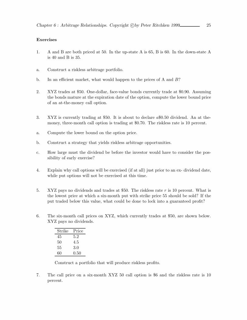
Exercises

1. A and B are both priced at 50. In the up-state A is 65, B is 60. In the down-state Ais 40 and B is 35.

a. Construct a riskless arbitrage portfolio.

b. In an efficient market, what would happen to the prices of A and B?

2. XYZ trades at $50. One-dollar, face-value bonds currently trade at $0.90. Assumingthe bonds mature at the expiration date of the option, compute the lower bound priceof an at-the-money call option.

3. XYZ is currently trading at $50. It is about to declare a$0.50 dividend. An at the-money, three-month call option is trading at $0.70. The riskless rate is 10 percent.

a. Compute the lower bound on the option price.

b. Construct a strategy that yields riskless arbitrage opportunities.

c. How large must the dividend be before the investor would have to consider the pos-sibility of early exercise?

4. Explain why call options will be exercised (if at all) just prior to an ex- dividend date,while put options will not be exercised at this time.

5. XYZ pays no dividends and trades at $50. The riskless rate r is 10 percent. What isthe lowest price at which a six-month put with strike price 55 should be sold? If theput traded below this value, what could be done to lock into a guaranteed profit?

6. The six-month call prices on XYZ, which currently trades at $50, are shown below.XYZ pays no dividends.

Strike Price45 5.250 4.555 3.060 0.50

Construct a portfolio that will produce riskless profits.

7. The call price on a six-month XYZ 50 call option is $6 and the riskless rate is 10percent.


a. Compute the lower bound on a six-month 50 put option. Assume the stock price is$52.

b. If the underlying stock declares a dividend of $1 two months prior to expiration, wouldthe lower bound increase, decrease, or remain the same? Explain.

8. XYZ trades at $60. The market price of an XYZ January 50 put is 1/16. The marketprice of the January 50 call is $11. Consider the strategy of buying the stock and putoption and selling the call. Compute the initial investment and explain why a profitequal to the strike price less the initial investment is guaranteed.

9. Given XYZ trades at $30, the riskless rate of return is 12 percent, and an at-the-moneycall option with six months to expiration is trading at $4.

a. Compute the price of a European put option.

b. By plotting a profit function, show that the payouts of a stock can be replicated by aportfolio containing the six-month at-the-money call, a short position in the put, andborrowing funds at the riskless rate. How much needs to be borrowed?

10. Using arbitrage arguments alone, show that an American call option cannot be valuedmore than a stock.

11. Explain why a European put option could have a negative time premium, while anAmerican put option could not.

12. Prove Property 15.

Documents

Chapter 6 Arbitrage Relationships for Call and Put Options · Chapter 6 Arbitrage Relationships for Call and Put Options ... Throughout this chapter we shall adopt the following notation