Embed Size (px)
Citation preview
1
CHAPTER 6 - Chemical Equilibrium I. Thermodynamics of Chemical Reactions.
A. Spontaneity of Chemical Reactions:
1. Thermodynamics can tell us:
a. direction of spontaneous change.
b. composition when equilibrium is reached.
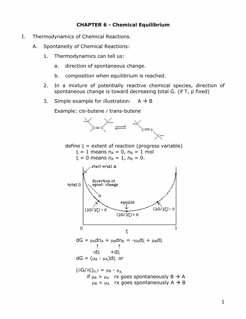
2. In a mixture of potentially reactive chemical species, direction of spontaneous change is toward decreasing total G. (if T, p fixed)
3. Simple example for illustration: A ! B
Example: cis-butene ⁄ trans-butene
define ξ = extent of reaction (progress variable) ξ = 1 means nA = 0, nB = 1 mol ξ = 0 means nA = 1, nB = 0.
dG = µAdnA + µBdnB = -µAdξ + µBdξ ↑ ↑ -dξ +dξ dG = (µB - µA)dξ or (∂G/∂ξ)p,T = µB - µA if µB > µA rx goes spontaneously B ! A µB < µA rx goes spontaneously A ! B
2
Equilibrium is reached when:
µB = µA or (∂G/∂ξ)p,T = 0
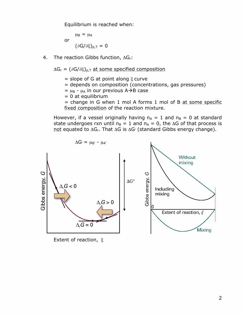
4. The reaction Gibbs function, ΔGr:
ΔGr = (∂G/∂ξ)p,T at some specified composition
= slope of G at point along ξ curve = depends on composition (concentrations, gas pressures) = µB - µA in our previous A!B case = 0 at equilibrium = change in G when 1 mol A forms 1 mol of B at some specific
fixed composition of the reaction mixture.
However, if a vessel originally having nA = 1 and nB = 0 at standard state undergoes rxn until nB = 1 and nA = 0, the ΔG of that process is not equated to ΔGr. That ΔG is ΔGθ (standard Gibbs energy change). ΔGθ = µBθ - µAθ
Extent of reaction, ξ
3
5. Exergonic vs endergonic reactions:
if a mixture of A and B at a specified composition has: ΔGr < 0, will proceed spont. in A --> B (said to be exergonic) ΔGr > 0, will proceed spont. in A <-- B (said to be endergonic) = 0, equilibrium
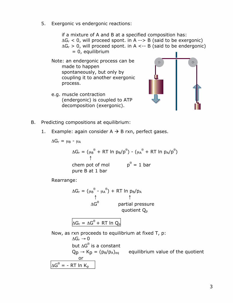
Note: an endergonic process can be made to happen spontaneously, but only by coupling it to another exergonic process.
e.g. muscle contraction
(endergonic) is coupled to ATP decomposition (exergonic).
B. Predicting compositions at equilibrium:
1. Example: again consider A ! B rxn, perfect gases.
ΔGr = µB - µA
ΔGr = (µBθ + RT ln pB/p
θ) - (µAθ + RT ln pA/p
θ)
↑
chem pot of mol pθ = 1 bar pure B at 1 bar
Rearrange:
ΔGr = (µBθ - µA
θ) + RT ln pB/pA ↑ ↑
ΔGθ partial pressure quotient Qp
ΔGr = ΔGθ + RT ln Qp
Now, as rxn proceeds to equilibrium at fixed T, p: ΔGr → 0
but ΔGθ is a constant Qp → Kp = (pB/pA)eq equilibrium value of the quotient or
ΔGθ = - RT ln Kp
4
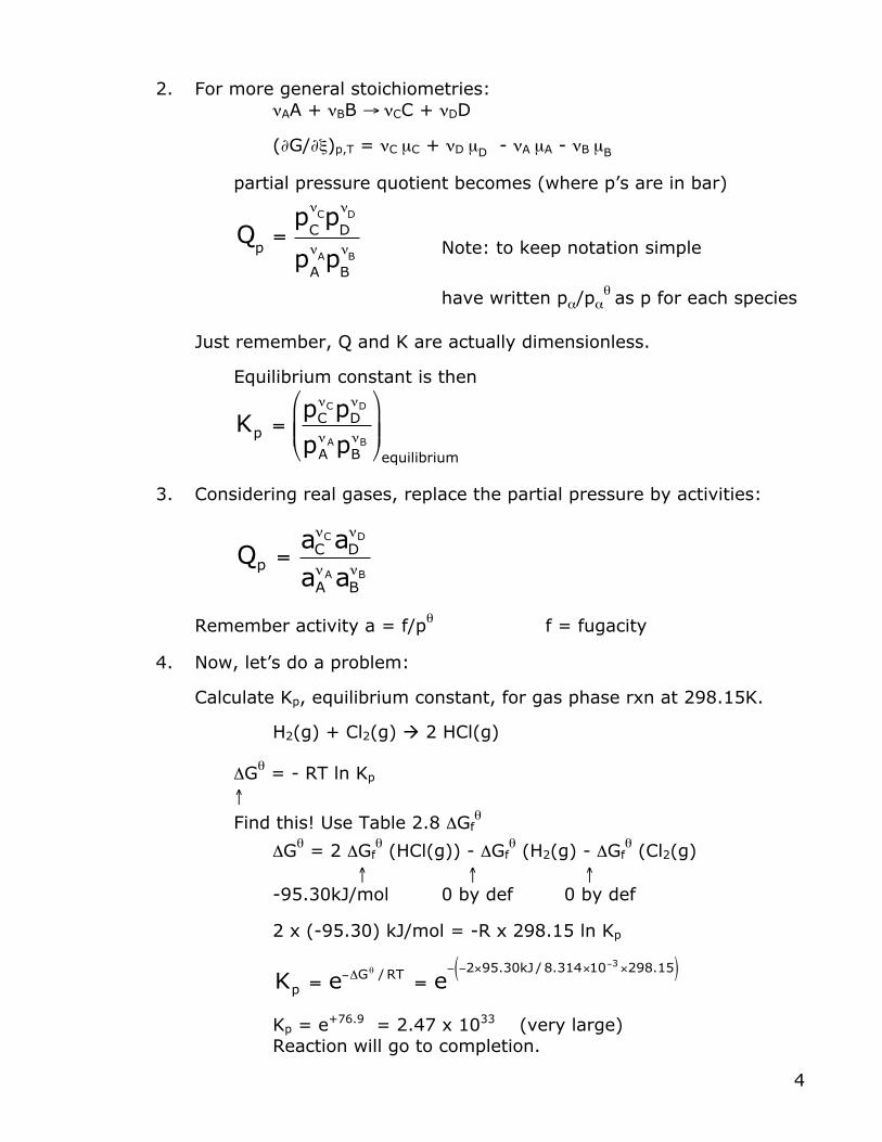
2. For more general stoichiometries: νAA + νBB → νCC + νDD
(∂G/∂ξ)p,T = νC µC + νD µD - νA µA - νB µB
partial pressure quotient becomes (where p’s are in bar)
Qp=pC
νCpD
νD
pA
νApB
νB Note: to keep notation simple
have written pα/pαθ as p for each species
Just remember, Q and K are actually dimensionless.
Equilibrium constant is then
€
Kp =pCνCpD
νD
pAνApB
νB
#
$ % %
&
' ( ( equilibrium
3. Considering real gases, replace the partial pressure by activities:
€
Qp =aCνC aD
νD
aAνA aB
νB
Remember activity a = f/pθ f = fugacity
4. Now, let’s do a problem:
Calculate Kp, equilibrium constant, for gas phase rxn at 298.15K.
H2(g) + Cl2(g) ! 2 HCl(g)
ΔGθ = - RT ln Kp ↑
Find this! Use Table 2.8 ΔGfθ
ΔGθ = 2 ΔGfθ (HCl(g)) - ΔGf
θ (H2(g) - ΔGfθ (Cl2(g)
↑ ↑ ↑ -95.30kJ/mol 0 by def 0 by def
2 x (-95.30) kJ/mol = -R x 298.15 ln Kp
€
Kp = e−ΔGθ / RT = e− −2×95.30kJ / 8.314×10−3 ×298.15( )
Kp = e+76.9 = 2.47 x 1033 (very large) Reaction will go to completion.
5
5. Practical expressions for equilibrium constants:
In general, Q and K = quotient of activities
Factor out activity coefficients:
Solution reactions, use aα = γα mα/mθ
↑ ↑ molality 1 molal
Q =mC
νCmD
νD
mA
νAmB
νB
"
#
$$
%
&
''γC
νCγD
νD
γA
νAγB
νB
"
#
$$
%
&
''
Q = QmQ
γ
and therefore:
K =mC
νCmD
νD
mA
νAmB
νB
"
#
$$
%
&
''equilib_mix
γC
νCγD
νD
γA
νAγB
νB
"
#
$$
%
&
''equilib_mix
K = KmK
γ
Often Kγ ≈ 1 so K ≈ Km
II. Response of Equilibria to Conditions. (response to changes in p or T)
A. Responses to pressure changes.
1. How Kp changes with pressure. It doesn’t!
ΔGθ = - RT ln Kp general expression ↑ ↑ stnd Kp independent Gibbs energy of pressure
2. How equilibrium compositions change with pressure. They do!
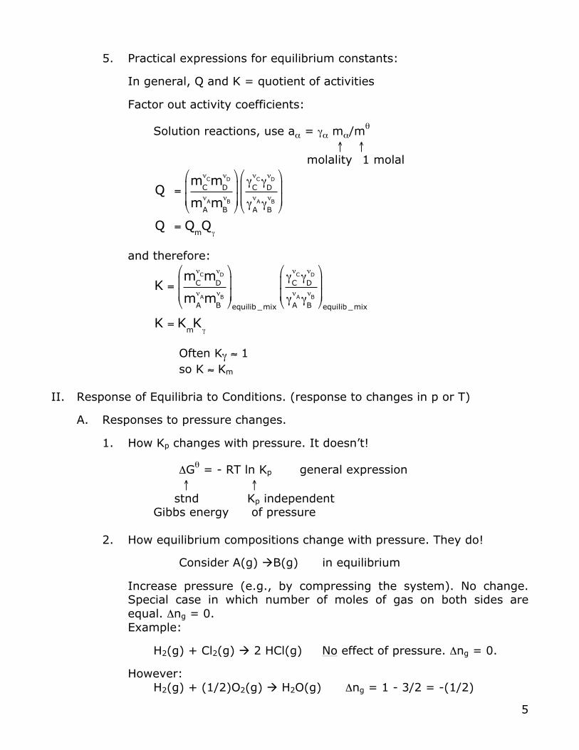
Consider A(g) !B(g) in equilibrium
Increase pressure (e.g., by compressing the system). No change. Special case in which number of moles of gas on both sides are equal. Δng = 0. Example:
H2(g) + Cl2(g) ! 2 HCl(g) No effect of pressure. Δng = 0.
However: H2(g) + (1/2)O2(g) ! H2O(g) Δng = 1 - 3/2 = -(1/2)
6
So here, an increase applied pressure will favor forward rxn, since this will reduce moles of gas. ~Le Chatelier’s principle
When a system at equilibrium is disturbed, it responds in a way
that tends to minimize the effect of the disturbance.
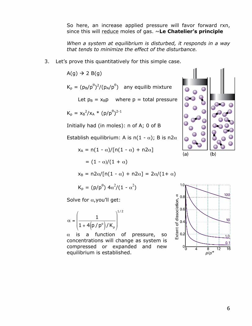
3. Let’s prove this quantitatively for this simple case. A(g) ! 2 B(g)
Kp = (pB/pθ)2/(pA/p
θ) any equilib mixture Let pB = xBp where p = total pressure
Kp = xB2/xA * (p/pθ)2-1
Initially had (in moles): n of A; 0 of B Establish equilibrium: A is n(1 - α); B is n2α xA = n(1 - α)/[n(1 - α) + n2α] = (1 - α)/(1 + α) xB = n2α/[n(1 - α) + n2α] = 2α/(1+ α)
Kp = (p/pθ) 4α2/(1 - α2) Solve for α,you’ll get:
€
α =1
1 + 4 p /po( ) /Kp
#
$
% %
&
'
( (
1/ 2
α is a function of pressure, so concentrations will change as system is compressed or expanded and new equilibrium is established.
7
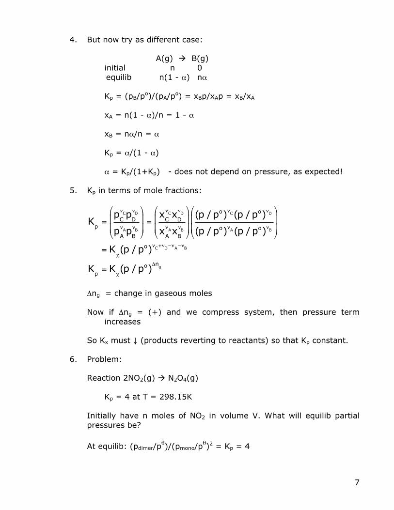
4. But now try as different case: A(g) ! B(g) initial n 0 equilib n(1 - α) nα Kp = (pB/po)/(pA/po) = xBp/xAp = xB/xA xA = n(1 - α)/n = 1 - α xB = nα/n = α Kp = α/(1 - α) α = Kp/(1+Kp) - does not depend on pressure, as expected!
5. Kp in terms of mole fractions:
Kp=pC
νCpD
νD
pA
νApB
νB
"
#
$$
%
&
''=xC
νCxD
νD
xA
νAxB
νB
"
#
$$
%
&
''(p / po)νC(p / po)νD
(p / po)νA(p / po)νB
"
#
$$
%
&
''
= Kχ(p / po)νC+νD−νA−νB
Kp= K
χ(p / po)
Δng
Δng = change in gaseous moles Now if Δng = (+) and we compress system, then pressure term
increases So Kx must ↓ (products reverting to reactants) so that Kp constant.
6. Problem:
Reaction 2NO2(g) ! N2O4(g) Kp = 4 at T = 298.15K Initially have n moles of NO2 in volume V. What will equilib partial pressures be?
At equilib: (pdimer/pθ)/(pmono/p
θ)2 = Kp = 4
8
Could also write: Kp = (xdimer/xmono
2)(p/pθ)-1 = 4 2NO2 ! N2O4 n 0 init moles n(1-2α) nα equil moles xdimer = α/(1-2α + α) = α/(1 - α) xmono = (1-2α)/(1 - α) p = pdimer + pmono = (ndimer + nmono)RT/V p = (α + 1 - 2α)n RT/V = (1 - α)n RT/V = (1 - α)pinit Use pθ = 1 bar; pinit ≡ nRT/V Kp = [α/(1-2α)2] pinit
-1 Rearrange and solve for α = number moles N2O4 formed when equilib. Will get a quadratic eqn. in α. α = (Kp pinit)(1 - 4α + 4α2) 0 = Kp pinit - (4 Kp pinit + 1)α + 4 Kp pinit α
2
α =4K
ppinit
+1( ) ± 4Kppinit
+1( )2− 4K
ppinit( )
2
8Kppinit
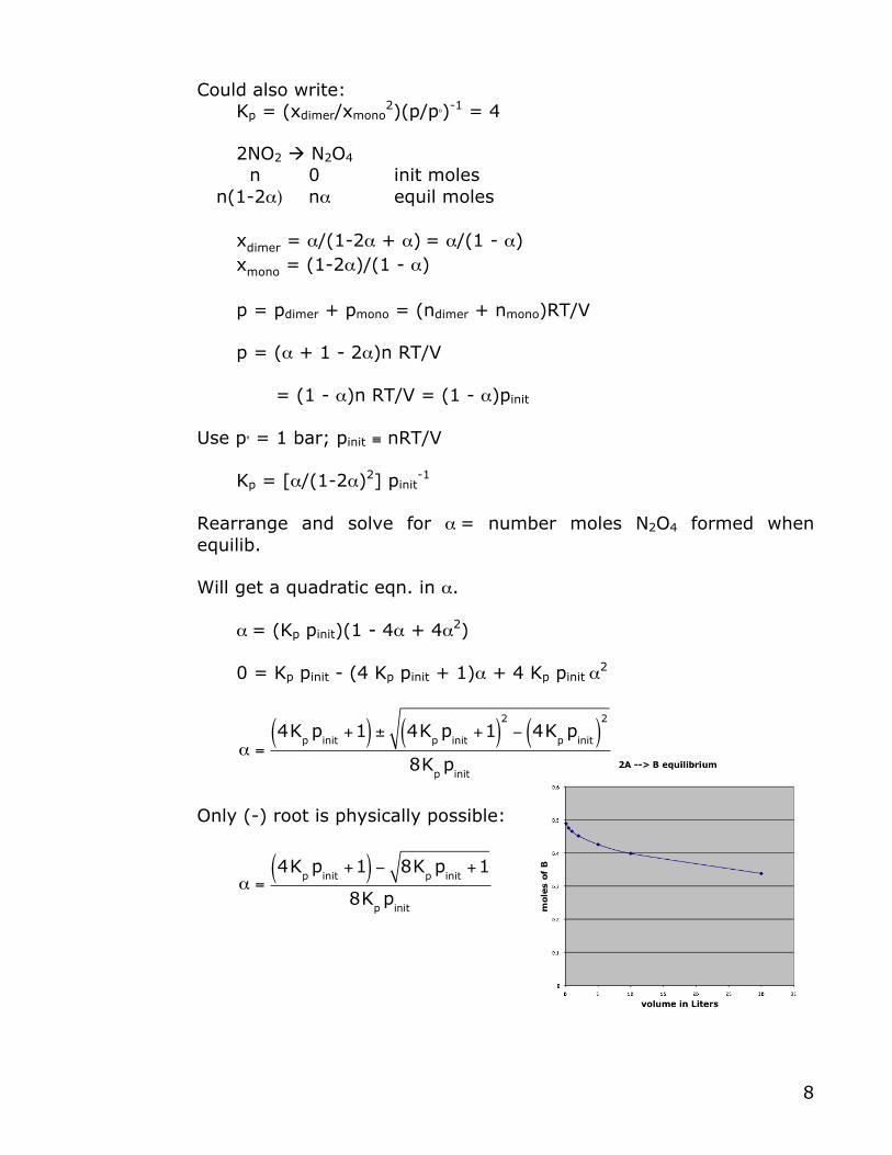
Only (-) root is physically possible:
α =4K
ppinit
+1( ) − 8Kppinit
+1
8Kppinit
9
B. The response of equilibrium to temperature. 1. Basic idea:
If A ! B + heat (exothermic) Then as T ↑, K ↓, equilibrium will shift back to reactants T ↓ K↑ Therefore, K is a sensitive function of T. Exothermic reactions, increased T favors reactants Endothermic reactions, increased T favors products
2. The van’t Hoff equation proves this:
Start with ΔGθ = - RT ln Kp
lnK = −ΔGo /RT
dlnKdT
= −1Rd(ΔGo / T)dT
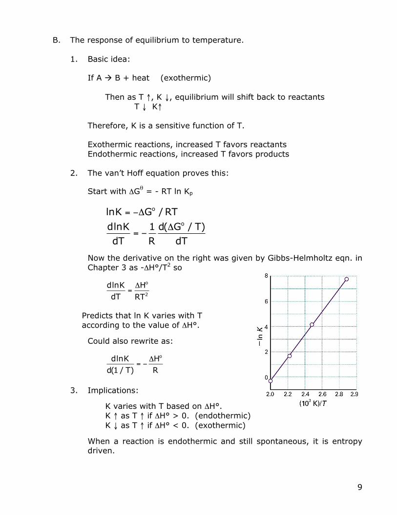
Now the derivative on the right was given by Gibbs-Helmholtz eqn. in Chapter 3 as -ΔH°/T2 so
dlnKdT
=ΔHo
RT2
Predicts that ln K varies with T according to the value of ΔH°.
Could also rewrite as:
dlnKd(1 / T)
= −ΔHo
R
3. Implications:
K varies with T based on ΔH°. K ↑ as T ↑ if ΔH° > 0. (endothermic) K ↓ as T ↑ if ΔH° < 0. (exothermic)
When a reaction is endothermic and still spontaneous, it is entropy driven.
10
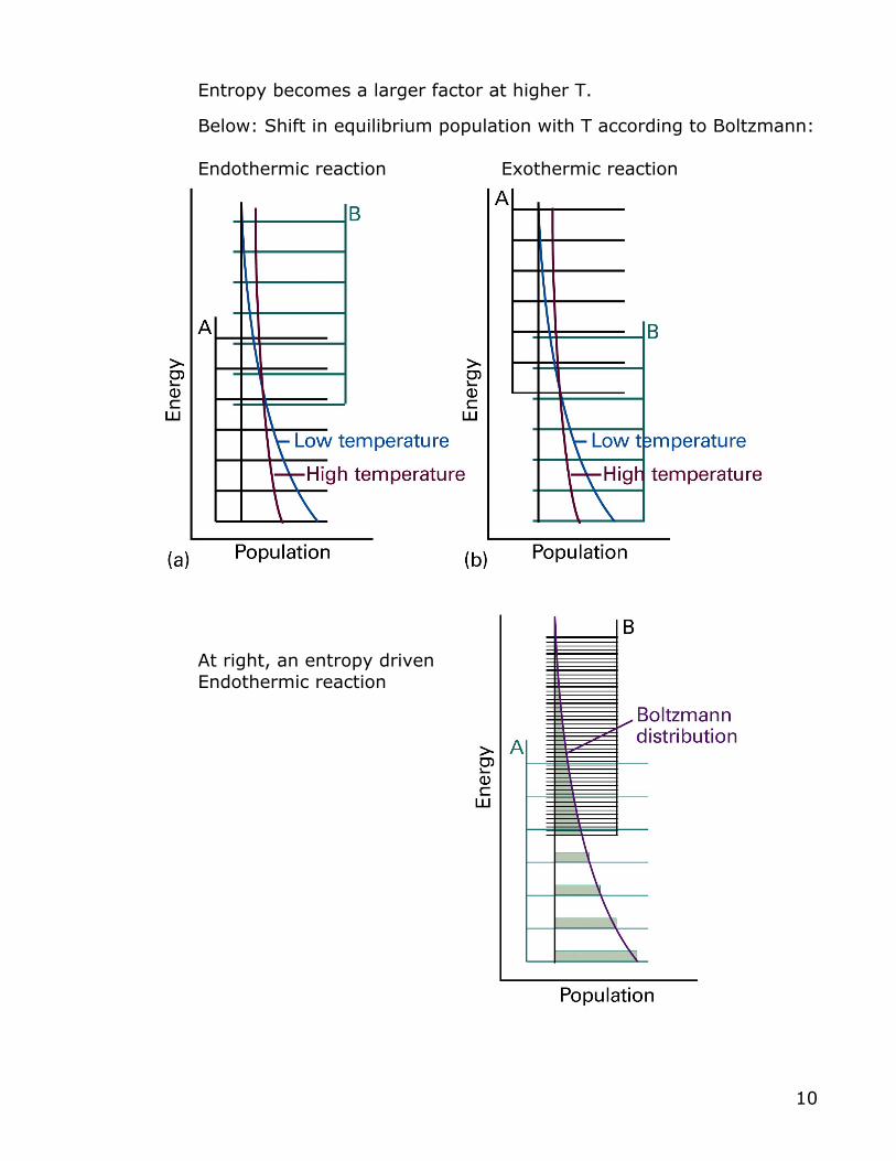
Entropy becomes a larger factor at higher T.
Below: Shift in equilibrium population with T according to Boltzmann: Endothermic reaction Exothermic reaction
At right, an entropy driven Endothermic reaction
11
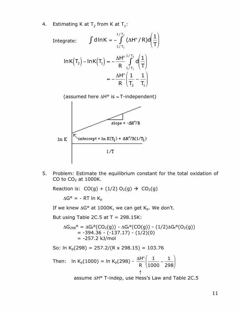
4. Estimating K at T2 from K at T1:
Integrate:
€
dlnK = − (ΔH° /R)d1T
$
% &
'
( )
1/ T1
1/ T2
∫∫
€
lnK T2( ) − lnK T1( ) ≈ − ΔH°
Rd
1T
%
& '
(
) *
1/ T1
1/ T2
∫
≈ −ΔH°
R1T2
−1T1
%
& '
(
) *
(assumed here ΔH° is ≈ T-independent)
5. Problem: Estimate the equilibrium constant for the total oxidation of CO to CO2 at 1000K.
Reaction is: CO(g) + (1/2) O2(g) ! CO2(g)
ΔG° = - RT ln Kp
If we knew ΔG° at 1000K, we can get Kp. We don’t.
But using Table 2C.5 at T = 298.15K:
ΔG298° = ΔGf°(CO2(g)) - ΔGf°(CO(g)) - (1/2)ΔGf°(O2(g)) = -394.36 - (-137.17) - (1/2)(0) = -257.2 kJ/mol
So: ln Kp(298) = 257.2/(R x 298.15) = 103.76
Then: ln Kp(1000) = ln Kp(298) -
€
ΔH°
R1
1000−
1298
$
% &
'
( )
↑ assume ΔH° T-indep, use Hess’s Law and Table 2C.5
12
ΔH° = -393.51 - (-110.53) - (1/2)(0) = -282.98 kJ/mol exothermic
lnKp1000( ) =
lnKp298( ) +282.98
8.314 ×10⁻³( ) 11000
−1298
#
$%%
&
'((
= 103.76 − 80.12
ln Kp(1000) = 23.6
Kp(1000) = e23.6 = 1.84 x 10¹⁰
Whereas Kp(298.15) = e103.76 = 1.15 x 1045
As expected, for exothermic reactions, Kp ↓ as T ↑.
6. For the gas phase dimerization reaction 2 NO2 ⇔ N2O4 use Table 2C.5 to calculate Kp at 298 and 600 K.
ΔGrx298( ) = 97.89 −2 ∗51.31 = −4.73
lnKp= −
ΔG°RT
= 1.908
Kp= e
− −4.73RT
"
#$$
%
&''= 6.74
lnKp600( ) = lnKp 298( ) − ΔH°
R1600
−1298
#
$%%
&
'((
ΔH° = 9.16 −2 ∗33.18 = −57.2kJ
mol
lnK
p600( ) = −4.88
Kp= 0.00759
13
III. Application to Equilibrium Electrochemistry.
A. Electrochemical Cells:
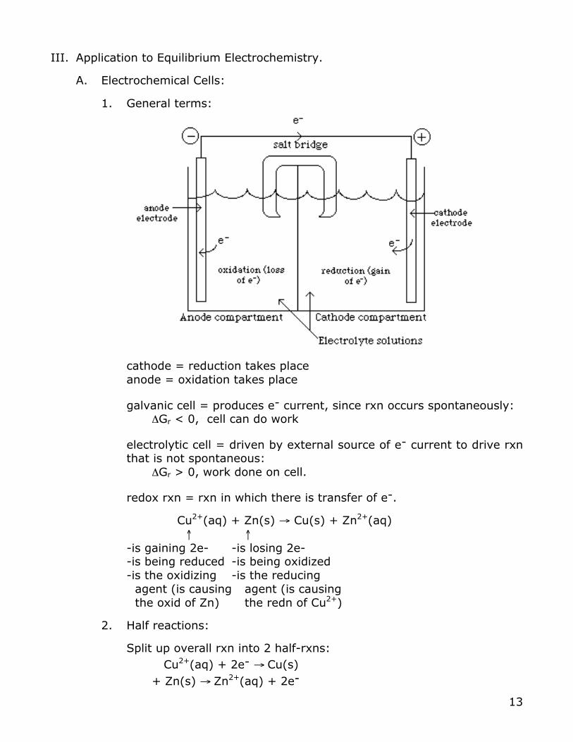
1. General terms:
cathode = reduction takes place anode = oxidation takes place
galvanic cell = produces e- current, since rxn occurs spontaneously: ΔGr < 0, cell can do work
electrolytic cell = driven by external source of e- current to drive rxn that is not spontaneous: ΔGr > 0, work done on cell.
redox rxn = rxn in which there is transfer of e-.
Cu2+(aq) + Zn(s) → Cu(s) + Zn2+(aq) ↑ ↑ -is gaining 2e- -is losing 2e- -is being reduced -is being oxidized -is the oxidizing -is the reducing agent (is causing agent (is causing the oxid of Zn) the redn of Cu2+)
2. Half reactions:
Split up overall rxn into 2 half-rxns: Cu2+(aq) + 2e- → Cu(s) + Zn(s) → Zn2+(aq) + 2e-
14
Or could write as difference of two reductions: Cu2+ + 2e- → Cu - [Zn2+ + 2e- → Zn]
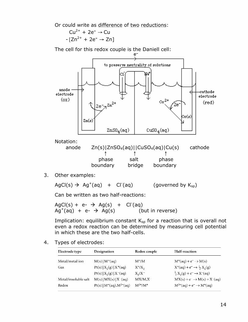
The cell for this redox couple is the Daniell cell:
Notation: anode Zn(s)|ZnSO4(aq)||CuSO4(aq)|Cu(s) cathode ↑ ↑ ↑ phase salt phase
boundary bridge boundary
3. Other examples:
AgCl(s) ! Ag+(aq) + Cl-(aq) (governed by Ksp)
Can be written as two half-reactions:
AgCl(s) + e- ! Ag(s) + Cl-(aq) Ag+(aq) + e- ! Ag(s) (but in reverse)
Implication: equilibrium constant Ksp for a reaction that is overall not even a redox reaction can be determined by measuring cell potential in which these are the two half-cells.
4. Types of electrodes:
15
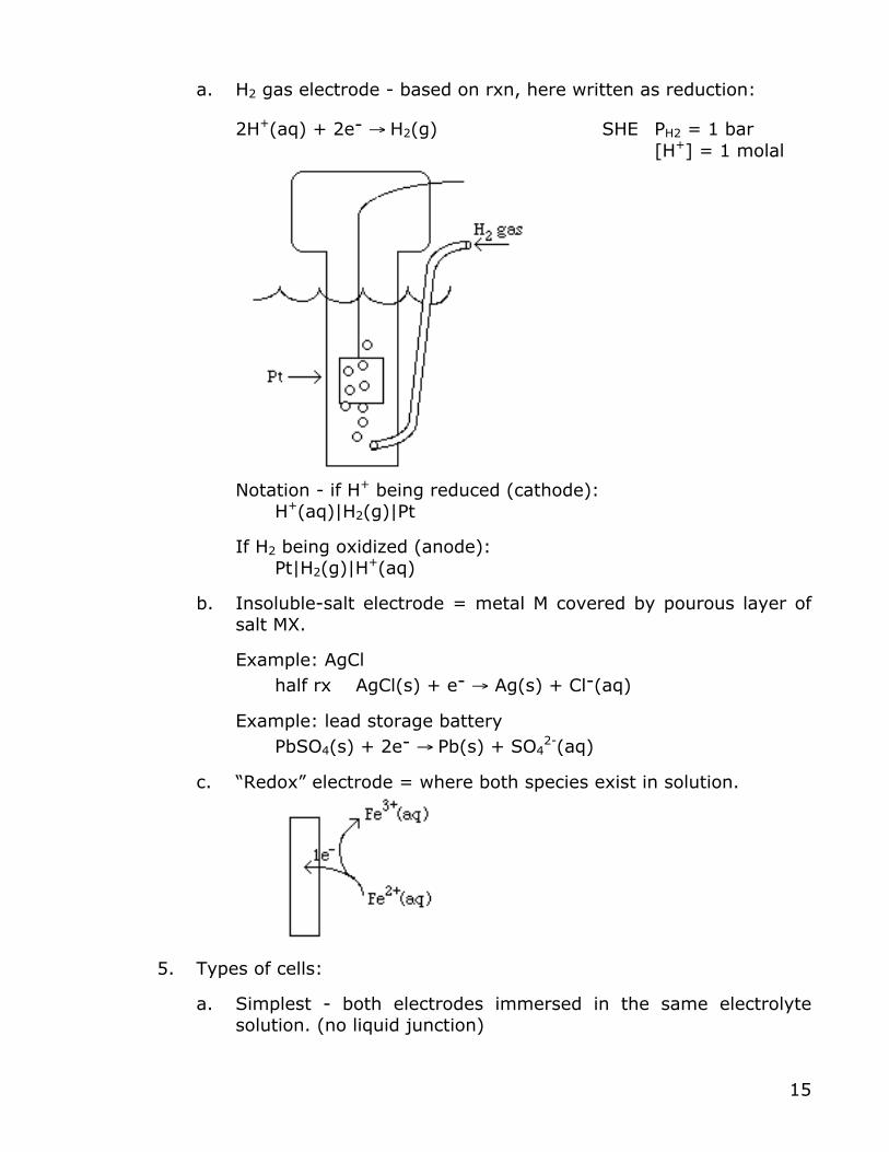
a. H2 gas electrode - based on rxn, here written as reduction:
2H+(aq) + 2e- → H2(g) SHE PH2 = 1 bar [H+] = 1 molal Notation - if H+ being reduced (cathode): H+(aq)|H2(g)|Pt
If H2 being oxidized (anode): Pt|H2(g)|H+(aq)
b. Insoluble-salt electrode = metal M covered by pourous layer of salt MX.
Example: AgCl half rx AgCl(s) + e- → Ag(s) + Cl-(aq)
Example: lead storage battery PbSO4(s) + 2e- → Pb(s) + SO4
2-(aq)
c. “Redox” electrode = where both species exist in solution.
5. Types of cells:
a. Simplest - both electrodes immersed in the same electrolyte solution. (no liquid junction)
16
Example: Hydrogen electrode & AgCl electrode both immersed in HCl(aq).
Pt|H2(g)|HCl(aq)|AgCl(s)|Ag
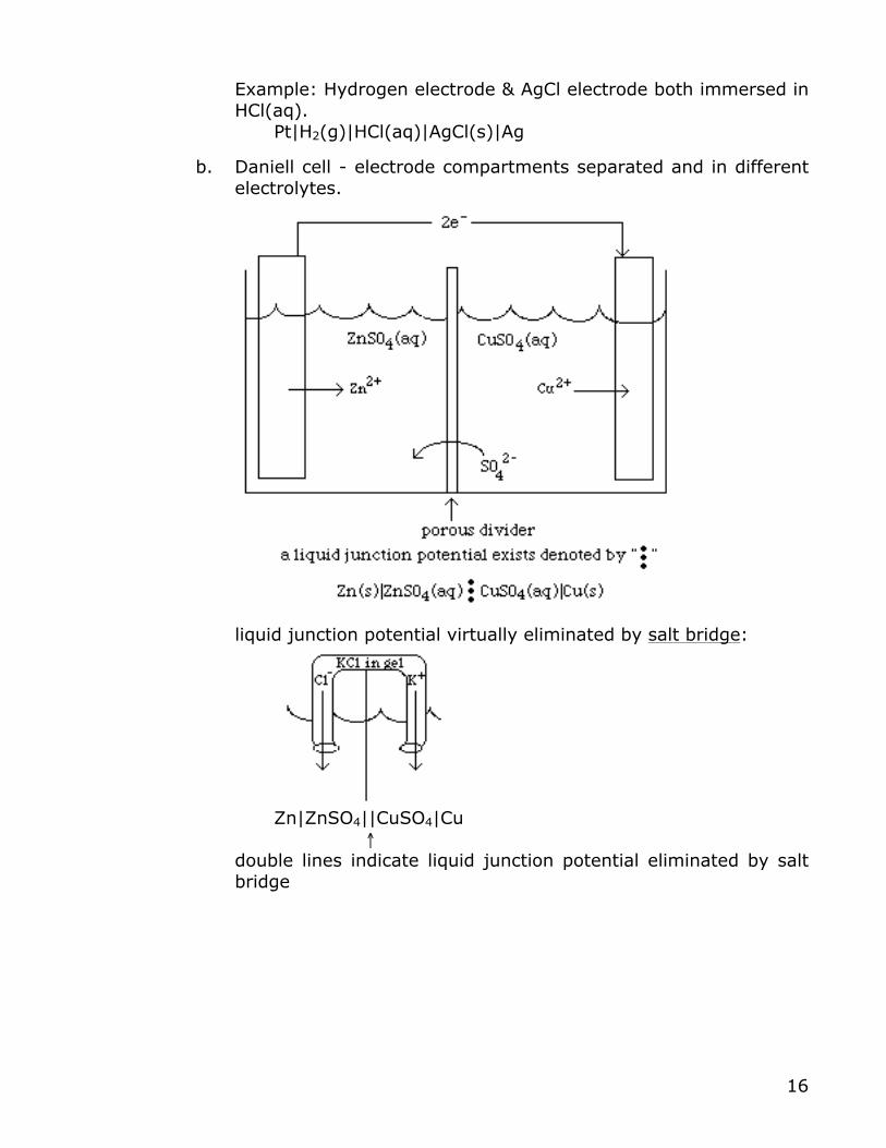
b. Daniell cell - electrode compartments separated and in different electrolytes.
liquid junction potential virtually eliminated by salt bridge:
Zn|ZnSO4||CuSO4|Cu ↑ double lines indicate liquid junction potential eliminated by salt
bridge
17
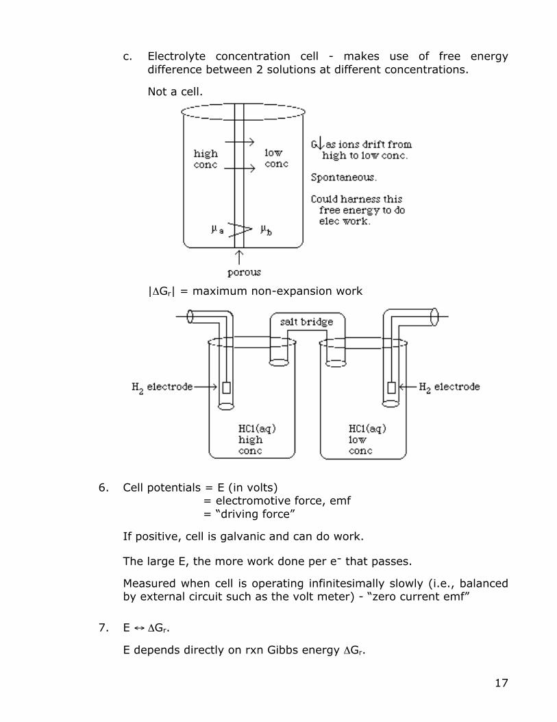
c. Electrolyte concentration cell - makes use of free energy difference between 2 solutions at different concentrations.
Not a cell.
|ΔGr| = maximum non-expansion work
6. Cell potentials = E (in volts) = electromotive force, emf = “driving force”
If positive, cell is galvanic and can do work.
The large E, the more work done per e- that passes.
Measured when cell is operating infinitesimally slowly (i.e., balanced by external circuit such as the volt meter) - “zero current emf”
7. E ↔ ΔGr.
E depends directly on rxn Gibbs energy ΔGr.
18
ΔGr = - νFE negative means ΔGr negative (spont) given E positive ν = moles of e- in balanced rxn; ν = 2 for Cu, Zn rxn F = Faraday constant (96485 Coul/mol); E = emf Remember: ΔGr = ΔG° + RT ln Q ↑ ↑(quotient of activities) = 0 at equilibrium Q = K at equilibrium > 0 if reverse rx is spont. Q > K < 0 if forward rx is spont. Q < K
8. Nernst Equation - variation of emf with concentrations (or activities, to be precise).
Start with: ΔGr = ΔG° + RT ln Q replace: ↓ ↓ -νFE = -νFE° + RT ln Q ↑ ↑ ↑activity quotient at existing conc. emf under emf in hypothet state existing conc when activities of conditions reactants & products are all 1
Rearrange:
E = E° - (RT/νF) ln Q
RT/F = 25.7 mV (millivolts) at 298.15K (25°C) E° = standard cell potential
What happens at equilibrium: Q → K
So: RTln Q → RTln K = -ΔG° = +νFE° E → 0
Could write, using equilibrium conditions:
0 = E° - RT/νF ln K
ln K = νFE°/RT
Thus can obtain K from cell potentials.
19
9. Concentration cell.
Can now see use of concentration gradients to perform emf work:
E = E° - RT/νF ln Q E° = 0
Pt|H2(g)|H+(aq, low conc)||H+(aq, high conc)|H2|Pt
Write out: H2 → 2H+(low) + 2e- 2H+(high) + 2e- → H2
Net rxn: 2H+(high) → 2H+(low) Q = a(H+(low conc))2/a(H+(high conc))2 ν = 2 Q < 1 ln Q = neg -RT/νF ln Q = positive E = E° + positive E > 0 ↑= 0
Problem: assume [H+] are sufficiently low that can replace activities by concentrations. Suppose [H+] in high conc part of cell is twice that in low conc part. Calculate emf.
E = 0 –(RT/νF) ln (1/2)2
ν = 2; RT/F = 25.7mV
= -(25.7/2) * 2 ln(1/2)
E = 17.8mV
10. Problem - calculate E of cell from Nernst eqn., use DH theory to get ion activities, use ΔGf’s to get E°.
Cell notation: Zn(s)|ZnSO4(aq, 0.002molal)||CuSO4(aq, 0.004 molal)|Cu(s)
Write out: Zn(s) → ZnSO4(aq) + 2e-
CuSO4(aq) + 2e- → Cu(s) + SO42-(aq)
Zn(s) + Cu2+(aq) → Zn2+(aq) + Cu(s)
E = E° - RT/νF ln Q ↑ desired quantity
20
ν = 2 RT/F = 25.7mV Q = a(Zn2+)/a(Cu2+)
E° = -ΔG°/νF ΔG° = ΔG°f(Zn2+(aq)) - ΔG°f(Cu2+(aq)) = -212.7 kJ/mol -147.1 +65.6 ΔGf of Cu(s) and Zn(s) = 0
E° = -(-212.7)/(2 * 96.485 kCmol-1) = 1.102V (Joul=Coul-Volt) a(solute) = γm/mθ a(Zn2+, 0.002 molal) = γ± (ZnSO4)* 0.002m/1m a(Cu2+, 0.004 molal) = γ± (CuSO4)* 0.004m/1m
DH theory: log γ± = - |Z+Z-|A√I = -|(+2)(-2)|.509√I I = (1/2)Σ Zi
2mi
I in ZnSO4 (0.002 molal) = (1/2){(+2)20.002 + (-2)20.002} ↑Zn2+ ↑SO4
2- = 0.008
I in CuSO4 (0.004 molal) = (1/2){(+2)20.004 + (-2)20.004} = 0.016
ZnSO4 log γ± = -|(+2)(-2)|.509√.008 = -0.182 γ± = 10-.182 = 0.657
CuSO4 log γ± = -|(+2)(-2)|.509√.016 γ± = 0.552
Q = a(Zn2+)/a(Cu2+) = (0.657 * 0.002)/(0.552 * 0.004) Q = 0.595
E = 1.102 – (0.0257V/2) ln 0.595 = 1.102 + .007 = 1.109 ↑ only 7 mV different than E°
11. Tabulated Reduction Potentials.
Consider reduction half-rxn: Ag+ + 1e- → Ag(s)
Impossible to measure E of this rxn by itself. Need a rx couple.
To tabulate E° for series of species then, let’s arbitrarily define: E° = 0 at all T for the reaction: 2H+(aq) + 2e- → H2(g)
21
i.e. electrode Pt|H2(g)|H+(aq) is called the Standard Hydrogen Electrode (SHE) H2(g) pressure = 1 bar
Now if cell Pt|H2(g)|H+(aq)||Ag+(aq)|Ag(s) has E° = +0.80V,
then Ag+ + e- → Ag redn pot is E° = +.80V
since E°(H2/H+) = 0
In general, overall E° of cell is: E°(cell) = E°(redn half-rxn) - E°(ox half-rxn)
12. Now, let’s examine Table 6D.1 in Appendix of Atkins - explain how to use.
13. Show how to predict spontaneous direction for a given redox couple. E° rxn Cu2+ + 2e- → Cu 0.337 (-) (Zn2+ + 2e- → Zn) -(-0.763) Cu2+ + Zn → Cu + Zn2+ Erx° = 1.100 volts Pb2+ + 2e- → Pb -.126 (-) (Zn2+ + 2e- → Zn) -(-0.763) Pb2+ + Zn →Pb + Zn2+ E° = -0.126 -(-0.763) = 0.637 volts
14. Predicting Keq:
Find E° by combining half-rxns.
Then ΔG° = -νFE° ↑ number of e- transferred as the overall rxn is written
Then ln Keq = -ΔG°/RT = νFE°/RT
22
B. Application of Reduction Potentials.
1. Electrochemical Series:
In list of Standard Reduction Potentials, the higher E° is, the more easily reduced. (top of chart) Things lower on the table are more easily oxidized.
E°total = E°reduced species - E°oxidized species ↑ ↑ higher one on lower one on the chart the chart (both E° are the listed reduction potentials)
Arranging in order of reducability = electrochem series. (Atkins Table 6.2)
2. Solubility Products:
salt MX(s) ! M+(aq) + X-(aq)
solub Ksp = a(M+)a(X-) (a = 1 for the pure solid) product
If s = solubility = molality of M+ or X- in saturated soln.
And if γ± ≈ 1 (very dilute, low solub) Ksp = (s/mθ)2 s = Ksp
1/2mθ
↑ 1 mol/kg
Determine from cell experiment:
Problem: Find s of AgCl from cell potential data at 25°C.
Strategy - find 2 half-reactions that, when combined, produce the reaction:
E° AgCl(s) + e- → Ag(s) + Cl-(aq) +0.22V (-) (Ag+(aq) + e- → Ag(s)) -(+.80V) AgCl(s) → Ag+(aq) + Cl-(aq)
E°total = +0.22 - 0.80 = -.58V
Now ΔG° = -RT ln Ksp ↑ ↑ of solub solub equil constant
23
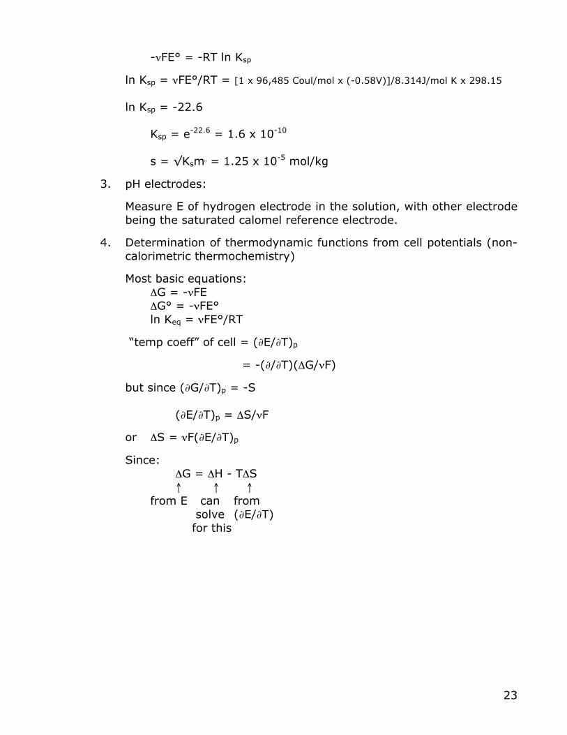
-νFE° = -RT ln Ksp
ln Ksp = νFE°/RT = [1 x 96,485 Coul/mol x (-0.58V)]/8.314J/mol K x 298.15 ln Ksp = -22.6 Ksp = e-22.6 = 1.6 x 10⁻¹⁰ s = √Ksmθ = 1.25 x 10⁻⁵ mol/kg
3. pH electrodes:
Measure E of hydrogen electrode in the solution, with other electrode being the saturated calomel reference electrode.
4. Determination of thermodynamic functions from cell potentials (non-calorimetric thermochemistry)
Most basic equations: ΔG = -νFE ΔG° = -νFE° ln Keq = νFE°/RT
“temp coeff” of cell = (∂E/∂T)p
= -(∂/∂T)(ΔG/νF)
but since (∂G/∂T)p = -S (∂E/∂T)p = ΔS/νF
or ΔS = νF(∂E/∂T)p
Since: ΔG = ΔH - TΔS ↑ ↑ ↑ from E can from solve (∂E/∂T) for this

24
Notes: