Embed Size (px)
Citation preview
180
CHAPTER 6
CLOSED LOOP STUDIES
Improvement of closed-loop performance needs proper tuning of
controller parameters that requires process model structure and the estimation
of respective parameters which are discussed in detail in the previous chapter.
The present chapter discusses the methods for the design of multi-loop control
strategy and tuning of controller parameters. In order to achieve desired
quality, specified output characteristics at the cost of spending optimum
inputs one needs to design a controller and run the plant under closed loop so
that optimal production is achieved under safe operation.
6.1 INTRODUCTION
Controllers for MIMO systems can be either multi-loop
(Controllers are designed only for diagonal elements of process models of
transfer function matrix) or multivariable (Controllers are designed for all the
elements of the MIMO transfer function matrix). Multi-loop control scheme
has an edge over multivariable as the former can work even if a single-loop
fails. In the presence of interactions between input/ output the process needs
to be decoupled and then multi-loop controllers can be designed. When
interaction effects produce a significant deterioration in control system
performance, decoupling control has to be considered. Thus multi-loop or
multivariable controller involves the objective of maintaining several
controlled variables at independent set points.

181
Many researchers have worked on design of multi-loop controllers
for MIMO systems. Luyben (1986) presented a simple practical approach to
the problem of finding reasonable controller settings for N SISO controllers in
Nth order which is a typical industrial multivariable process. Loh et al (1993)
proposed the autotuning of multi-loop PI controller. This procedure is the
combination of sequential loop closing and relay tuning often used for tuning
single PI/ PID controllers. Huang et al (1993) proposed and implemented
PID controllers with the form of no proportional kick. Shen et al (1994)
proposed multivariable automatic tuning that performs the identification-
design procedure in a sequential manner which discusses the concept of
multivariable autotuner and the underlying theory for sequential design and
sequential identification employed in autotuning procedure. Palmor et al
(1995) proposed the automatic tuning of decentralized PID controllers for
TITO processes. Huang et al (2000) derived tuning rule from inverse based
PID controllers. Toh et al (2002) proposed a methodology for autotuning
decentralized proportional-integral-derivative (PID) controllers for
multivariable systems. Lee et al (2004) proposed a tuning method for multi-
loop PID controllers by extending the generalized IMC PID tuning method
for SISO systems. Liu et al (2005) proposed an analytical multi-loop
controller design for industrial and chemical 2-by-2 processes with time
delays. Vu et al (2008) proposed a new analytical method based on direct
synthesis approach for design of multi-loop PID controllers. This method is
aimed to achieve desired closed loop response for MIMO systems with
multiple time delays. Lin et al (2009) proposed a systematic procedure to
design multivariable controllers that have options for selective decoupling of
different structures (e.g. full or partial decoupler). Vu et al (2010) proposed a
novel method for independent design of multi-loop PI/ PID controllers. The
idea of an effective open-loop transfer function (EOTF) is introduced to
decompose multi-loop control system into a set of equivalent independent
single-loops. Veronesi and Visoli (2011) proposed a new automatic tuning

182
technique for multi-loop PID controllers applied to MIMO systems. Jeng et
al (2011) proposed the methods including model identification, controller
monitoring and controller retuning which in turn combined to develop an
intelligent control systems. Rajapandiyan and Chidambaram (2012) proposed
a method for the independent design of PI/ PID controllers based on
equivalent transfer function (ETF) model of individual loops and simplified
decoupler matrix.
6.2 DIFFERENT CONTROL DESIGN STRATEGIES
MIMO systems came into use in chemical industries as the
processes were redesigned to improve efficiency. Multivariable control
involves the objective of maintaining several controlled variables at
independent set points. Interaction between inputs and output cause a
manipulated variable to affect more than one controlled variable. The various
control schemes studied here are decentralized, centralized and decoupled
systems. In decentralized structure diagonal controllers are used hence, result
in system having n controllers whereas in the centralized control systems
having n x n controllers. In decoupled systems the process interactions are
decoupled before they actually reach and affect the processes.
6.2.1 Centralized Structure
Centralized control scheme is a full multivariable controller where
the controller matrix is not a mere diagonal one. The decentralized control
scheme is preferred over the centralized control scheme mainly because the
control system has only n manipulated signals controlling n output variables,
and the operator can easily understand the control loops. However, the design
methods of such decentralized controllers require first pairing of input-output
variables whereas tuning of controllers requires trial and error steps. The
centralized control system requires n x n controllers for controlling n output

183
variables using n manipulated variables. While calculating the control action
using computer, the problem of requiring n x n controllers does not exist. The
advantage of centralized controller is easy to tune even with the knowledge of
steady state gain matrix alone thereby multivariable PI controllers can be
easily designed.
For the centralized structure, Internal model control-proportional
integral tuning is adopted based on the studies and recommendations of
Reddy et al (1997) on tuning of centralized PI controllers for a Multi-stage
flash desalination plant using Davison, Maciejowski and Tanttu-Lieslehto
methods.
The IMC-PID tuning relations are used in tuning the controller.
When a first order system is in the formp
p
p 1
D sk es
, the PI controller settings are
as follows:
C
p
Kk l
(6.1)
pI (6.2)
where p pmax 1/ 0.7 ,0.2l D
These tuning relations are derived by comparing IMC control with
the conventional PID controller and thereby formulating the equations to
determine the proportional gain and integral time.

184
6.2.2 Decentralized Structure
In spite of developments in advanced controller synthesis for
multivariable controllers, decentralized controller remain popular in industries
because of the following reasons:
1. Decentralized controllers are easy to implement.
2. They are easy for operators to understand.
3. The operators can easily retune the controllers for change in
process conditions.
4. Some manipulated variables may fail. Tolerances of such
failures are easily incorporated into the design of
decentralized controllers than the full controllers.
5. The control system can be bought gradually into service
during process start up and taken gradually out of service
during shut down.
The design of decentralized control system consists of two main
steps:
Step 1 control structure selection
Step 2 design of SISO controller for each loop.
In decentralized control of multivariable systems, the system is
decomposed into number of subsystems and individual controllers are
designed for each subsystem.

185
For tuning of controller, Biggest Log Modulus Tuning (BLT)
method is used (Luyben, 1986), which is an extension of Multivariable
Nyquist Criterion and gives satisfactory response. Detuning factor F (typical
values are said to vary between 2 and 5) is chosen so that closed-loop log
modulus Lcmmax >= 2n,
cmw20log
1+wL = (6.3)
( )p cw 1 det I G G= - + + (6.4)
where GC is n x n diagonal matrix of PI controller transfer functions, Gp is n x
n matrix containing process transfer functions relating n controlled variables
to n manipulated variables.
Now the PI controller parameters are given as:
CiZ-NCi
KK F= (6.5)
Ii IiZ-NF (6.6)
where i stands for individual transfer function component, CiZ-NK and IiZ-N are
Ziegler-Nichols tuning parameters. These parameters are calculated from the
system perturbed in closed loop by relay of amplitude h, reaches a limit cycle
whose amplitude a and period of oscillation Pu. These parameters are
correlated with the ultimate gain (Ku) and frequency ( u) by the following
relationships:
4u
hKa
(6.7)

186
uu
2P
(6.8)
Detuning factor F determines the stability of each loop. The larger
the value of F more stable the system is but the set point and load responses is
sluggish. This method yield settings give a reasonable compromise between
stability and performance in multivariable systems.
The decentralized scheme is more advantageous in fact that the
system remains stable even when one controller goes down and easier to tune
because of less number of tuning parameters. However, pairing analysis
needs to be done as n! pairings between input/ output.
6.2.3 Decoupled Structure
This structure has additional elements called decouplers to
compensate for interaction phenomenon. When RGA shows strong interaction
then a decoupler is designed. However, decouplers are designed only for
order less than 3 as the design procedure becomes more complex as the order
increases.
The BLT (Luyben, 1986) procedure of tuning the decentralized
structure follows the generalized way for all n x n systems as mentioned
above. The centralized controllers are tuned using IMC-PI tuning relations
which are appropriately selected for first order and second order systems.
The decoupled structure adopts the various methods like partial,
static and dynamic decoupling to produce the best results. The design
equations for general decoupler for n x n systems are conveniently
summarized using matrix notations, defined as follows:

187
Transfer function matrix, 11 1n
n1 nn
G s G sG
G s G s
Decoupler matrix, 11 1n
n1 nn
D s D sD
D s D s
Diagonal matrix of decoupler, sH
sHsH
H
33
22
11
...0......0...
1
n
...u
uu
; 1
n
...M
MM
; 1
n
...y
yy
Manipulated variable (new) Manipulated variable (old) Output variable
For a decoupled multivariable system output can be written as:
GMy (6.9)
M=Du (6.10)
Equation (6.10) becomes:
GDy u (6.11)
Equation (6.11) becomes:
Hy u (6.12)
where,
GD=H (6.13)

188
(or) -1D=G H (6.14)
which defines the decoupler.
For 2-by-2 system, equations are derived for decouplers by taking
that loop as well as other interacting loops into account.
The scope of the discussion is the decentralized PI controller for
MIMO systems and the closed loop responses for set point tracking using
BLT tuning and IMC-PID Laurent series. The illustrations of decentralized
PI controllers are given in the following section using BLT tuning.
6.3 BIGGEST LOG MODULUS TUNING
Luyben proposed BLT tuning involves the following four steps:
Step 1 : Calculate the Ziegler-Nichols settings for each individual
loop. The ultimate gain and ultimate frequency of each
diagonal transfer function Gjj(s) are calculated in the classical
way. To do numerically, a value of frequency, is guessed.
The phase angle is calculated and the frequency is varied to
find the point where the Nyquist plot of Gjj crosses the
negative real axis (the phase angle is -180 degrees). The
frequency where it occurs is u. The reciprocal of the real part
of Gjj is the ultimate gain.
Step 2 : Detuning factor F is assumed which is always greater than 1.
Typical values are between 1.5 and 4. The gain of all
feedback controllers KCi are calculated by assuming Ziegler-
Nichols gain KZNi by the factor F.
ZNiCi F
KK

189
where, uiZNi 2.2KK
Then all feedback controller reset times Ii are calculated by
multiplying the Z-N reset times ZNi by the same factor F.
Ii ZNiF
where uiZNi 1.2P
The F factor can be considered as detuning factor which is
applied to all loops. Larger the value of F more stable the
system will be but more sluggish will be the set point and load
responses. The method yield settings that give a reasonable
compromise between stability and performance in
multivariable systems.
Step 3 : Using the guessed value of F and the resulting controller
settings, a multivariable nyquist plot of scalar function
Mi 1 det iW I G B is made. The point (-1, 0)
is closer to this contour then the system is closer to instability.
Therefore the quantity w1+w will be similar to closed loop
servo transfer function for SISO loop MM
B1+ B
GG . Based
on intuition and empirical grounds, multivariable closed loop
log modulus Lcm is defined.
cm 20log1
wLw
The peak in the plot of Lcm over the entire frequency range is
the biggest log modulus Lcmmax.

190
Step 4 : The F factor is varied until Lcmmax is equal to 2N. Where N is
the order of the system. For N=1 in SISO case, the familiar
+2dB max closed loop log modulus criterion is obtained. For
a 2-by-2 system, a +4dB value of Lcmmax is used and for 3-by-3
system a +6dB; hence forth.
An example given here is 2-by-2 MIMO system (WB column) with
transfer function matrix as in Equation (2.1).
Step 1: The ultimate gain and ultimate frequency for loop 1 and loop 2 are
Ku1 = 2.112, Pu1 = 3.9 and Ku2 = -0.418, Pu2 = 11.04. Using Ziegler-
Nichols settings the following controllers are obtained for loop 1 and
loop 2 that are KC1,ZN 11,ZN = 3.25 and KC2,ZN = 0.19,
12,ZN = 9.2.
Step 2: Assuming, F = 2.55.
Step 3: The F factor is varied until Lcmmax is equal to 4 for 2-by-2 MIMO
systems.
This empirically determined BLT criterion is tested on ten
multivariable distillation columns, varying from 2-by-2 system upto 4-by-4
MIMO systems (Luyben, 1986).
6.4 IMC PID LAURENT TUNING
IMC-PI controller parameters are derived by equating the closed
loop response to desired closed-loop response involving user defined tuning
in process transfer function. Controller synthesis procedure using desired
closed loop response involves synthesis of coefficient terms s0, s-1 and s1 in

191
PID parallel structure are discussed briefly by Panda (2009) in section 4.3.1.
Thus, the IMC-PI controller parameters for FOPDT processes are computed
using the following expressions:
2
pII p
p p p
;C
DK
k D D
6.5 RESULTS AND DISCUSSION
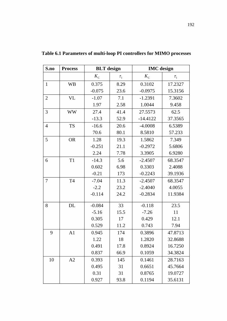
The parameters of multi-loop controllers using IMC and BLT
design for MIMO processes are listed in the following Table 6.1.
192
Table 6.1 Parameters of multi-loop PI controllers for MIMO processes
S.no Process BLT design IMC design CK I CK I
1 WB 0.375 -0.075
8.29 23.6
0.3102 -0.0975
17.2327 15.3156
2 VL -1.07 1.97
7.1 2.58
-1.2391 1.0044
7.3602 9.458
3 WW 27.4 -13.3
41.4 52.9
27.5573 -14.4122
62.5 37.3565
4 TS -16.6 70.6
20.6 80.1
-4.0008 8.5810
6.5389 57.233
5 OR 1.28 -0.251 2.24
19.3 21.1 7.78
1.5862 -0.2972 3.3905
7.349 5.6806 6.9280
6 T1 -14.3 0.602 -0.21
5.6 6.98 173
-2.4507 0.3303 -0.2243
68.3547 2.4088
39.1936 7 T4 -7.04
-2.2 -0.114
11.3 23.2 24.2
-2.4507 -2.4040 -0.2834
68.3547 4.0055
11.9384
8 DL -0.084 -5.16 0.305 0.529
33 15.5 17
11.2
-0.118 -7.26 0.429 0.743
23.5 11
12.1 7.94
9 A1 0.945 1.22
0.491 0.837
174 18
17.8 66.9
0.3896 1.2820 0.8924 0.1059
47.8713 32.8688 16.7250 34.3824
10 A2 0.393 0.495 0.31
0.927
145 31 31
93.8
0.1461 0.6651 0.8765 0.1194
28.7163 45.7664 19.0727 35.6131

193
To evaluate the output control performance, it is considered a unit
setpoint change of all control loops one by one and the integral square error
ISE ( i i ie y r ) used to evaluate the control performance.
2i
0
ISE e dt (6.15)
The simulation results and ISE values are given in Figures 6.1 to
6.10. The results show that IMC design provides better performance than
BLT design.
Figure 6.1 Step response and ISE values of multi-loop PI controllers
for WB column (solid line: IMC design; dashed line: BLT
design)

194
Figure 6.2 Step response and ISE values of multi-loop PI controllers
for VL column (solid line: IMC design; dashed line: BLT
design)

195
Figure 6.3 Step response and ISE values of multi-loop PI controllers
for WW column (solid line: IMC design; dashed line: BLT
design)

196
Figure 6.4 Step response and ISE values of multi-loop PI controllers
for TS column (solid line: IMC design; dashed line: BLT
design)

19
Figure 6.5 Step response and ISE values of multi-loop PI controllers for OR column (solid line: IMC design; dashed
line: BLT design)

Figure 6.6 Step response and ISE values of multi-loop PI controllers for T1 column (solid line: IMC design; dashed
line: BLT design)

Figure 6.7 Step response and ISE values of multi-loop PI controllers for T4 column (solid line: IMC design; dashed
line: BLT design)

Figure 6.8 Step response and ISE values of multi-loop PI controllers for DL column (solid line: I
line: BLT design)

Figure 6.9 Step response and ISE values of multi-loop PI controllers for A1 column (solid line: IMC design; dashed
line: BLT design)

Figure 6.10 Step response and ISE values of multi-loop PI controllers for A2 column (solid line: IMC design; dashed
line: BLT design)

203
6.6 OPTIMAL CONTROL DESIGN
The main objective of the present work is to capture the disturbance
dynamics thereby measure the interaction in terms of area under the closed
loop undesired response. The goal is to minimize the interaction by using
medium-scale algorithm with termination tolerances for step and objective
function in the order of 0.001. The optimization gives the solution for
proportional and integral gains (KC, KI) of the controller after 73 function
evaluations.
6.6.1 Parameter Optimization
The performance of closed-loop system is measured with single
scalar quantity performance index. Performance of each loop needs to be
better or improved at the cost of spending optimal/ minimum inputs. Thus the
problem is to formulate performance criteria that will lead to find optimal
solution of manipulated inputs. It needs to determine control configuration
selection and the free parameters of controller that optimizes the performance
index. A linear 2-by-2 MIMO process is considered to formulate
performance criteria. The optimal controller parameters found from the
solution will be used to retune the loops so as to minimize loss through
undesirable response and unnecessary disturbance through undesired loops.
A commonly used performance criterion is the area under the
regulatory response which is given by:
20
J y t dt (6.16)
This criterion has good mathematical track ability properties which
is acceptable in practice as a measure of system performance. Smaller the

204
value J results in small overshoot in the system. Since, the integration is
carried out ov all error lasting for
long time and thus results in small settling time. Also, a finite J implies that
the steady state error is zero.
Therefore, a more realistic performance index is of the form:
20
J y t dt subject to the following constraint on control signalu t , max
u t M for some constant M M determined by the
linear range of plant.
2u t is a measure of instantaneous rate of energy expenditure. To
minimize energy expenditure: 2
0
u t dt .
To replace the performance criterion the following quadratic
performance index as:
2 2
0
J e t u t dt (6.17)
To allow greater generality, a real positive constant can be
inserted to obtain the performance criterion J.
2 2
0
J e t u t dt (6.18)
By adjusting the weighting factor , one can weight the relative
importance of the system error and the expenditure in energy. Increasing the
by giving sufficient weight to control effort, the amplitude of the control

205
signal which minimizes the overall performance index which may be kept
within practical bounds although at the expenses of increased system error.
In this work, the main intention is to show the amount of interaction
obtainable in area calculation of closed loop undesirable/ regulatory
responses. For a general MIMO systems cost is minimized by changing the
input control signal, u. The control pairing which needs the least area to
fulfill its control targets will be the most efficient control pairing.
The design approach based on parameter optimization consists of
the following steps:
Step 0 : Compute the performance index (J) as a function of free
parameters k1, k2 kn, of the system with fixed configuration.
1 2 nJ J , ...k k k (6.19)
Step 1 : Determine the solution set ki of the equations
i
J 0; 1,2...nk
i (6.20)
Equation (6.17) gives the necessary conditions for J to be
minimum. From the solution set of these equations, find the
subset that satisfies the sufficient conditions which requires
that hessian matrix given is positive definite.
2 2 2
21 2 1 n1
2 2 2
22 1 2 n2
2 2 2
2n 1 n 2 n
J J J....
J J J....
. . . .
J J J....
k k k kk
H k k k kk
k k k k k

206
Since, 2 2
i j j i
J Jk k k k
the matrix H is always symmetric.
Step 2 : If there are two or more sets of ki satisfying the necessary and
sufficient conditions for minimization of J, then compute the
corresponding J for each set. The set which gives the smallest
J is optimum set.
In this work, the performance of the control system can be
adequately specified in terms of settling time, overshoot and steady state
error. Thus, the performance index can be chosen as
J k1 (settling time) + k2 (overshoot) + k3 (steady state error) (6.21)
In this work, the performance index which includes the undesirable
system characteristics and in addition good mathematical track ability are
presented. The performance indexes often involve integrating closed loop
regulatory response when the system is subjected to a standard disturbance
such as a step. The system whose design minimizes the selected performance
index on controller configuration is the optimal.
6.6.2 Monitoring of Closed Loop Undesired Responses and Redesign
of Controllers
The optimization toolbox routine offers a choice of algorithms. For
constrained minimization, minimax, goal attainment and semi-infinite
optimization, variations of sequential quadratic programming are used.
Nonlinear least squares problem uses the gauss-newton and levenberg-
marquardt methods.
To optimize the control parameters in simulink model optsim.mdl
(This model can be found in the optimization toolbox optim directory) which

207
includes nonlinear process plant (Equation 2.11) modeled as a simulink block
diagram. The problem is to design a feedback control law that tracks unit step
input to the system. One way to solve this problem is to minimize the error
between the output and the input signal. The variables are parameters of PI
controllers. The routine lsqnonlin is used to perform a least squares fit.
The function tracklsq must run the simulation. The simulation can be run
either in the base workspace or in current workspace. To run the simulation
in optsim, the variables KP, KI, a1 and a2 (a1 and a2 are variables in the plant
block) must be defined. KP and KI are the variables that are optimizing here.
The simulation is performed using fixed-step fifth-order method to 100
seconds.
The controller settings before and after optimization are tabulated
in Table 6.2:
Table 6.2 Controller parameters and area under undesired response for
coupled tanks system
Controller parameters
Before optimization
After optimization
ck 28.9520 41.9656
I 1.4476 0.0215
Area Before optimization
After optimization
2793.2 2655.2
With these controller settings, the closed loop undesired responses
before and after optimization is shown in Figure 6.11.

208
Figure 6.11 Closed loop undesired responses
6.6.3 Performance measure
Control effort calculated using this objective function is optimum
that saved energy. Thus, for the coupled tanks system gain optimum is
calculated as:
Gain optimum = 2793.2 2655.2 *100 4.95%2793.2
Optimum gain in this coupled tanks system is 5% when the
disturbance is 10%, thus the control effort is calculated using this objective
function which is found to be optimum that saved energy. Hence, the
optimized control signal has saved 5% of utility in this particular coupled
tanks system.
209
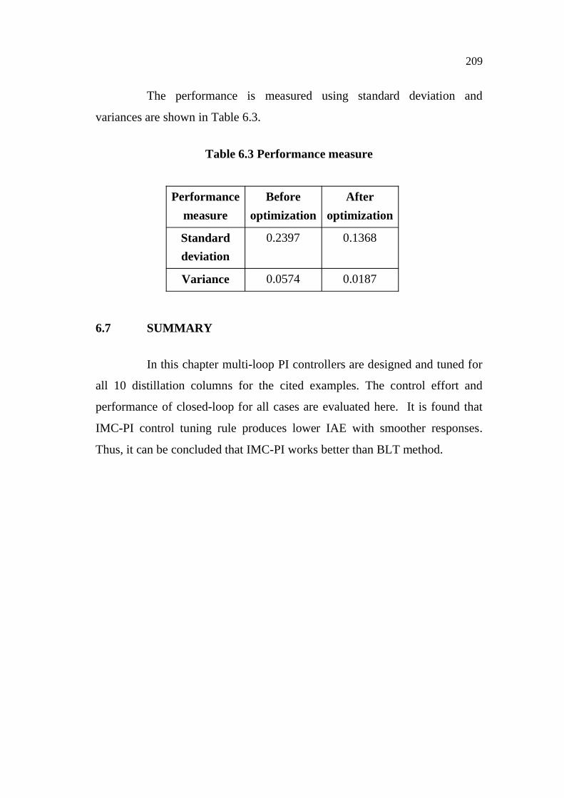
The performance is measured using standard deviation and
variances are shown in Table 6.3.
Table 6.3 Performance measure
6.7 SUMMARY
In this chapter multi-loop PI controllers are designed and tuned for
all 10 distillation columns for the cited examples. The control effort and
performance of closed-loop for all cases are evaluated here. It is found that
IMC-PI control tuning rule produces lower IAE with smoother responses.
Thus, it can be concluded that IMC-PI works better than BLT method.
Performance measure
Before optimization
After optimization
Standard deviation
0.2397 0.1368
Variance 0.0574 0.0187


![Closed loop Urbanism [Autosaved]](https://img.pdfslide.net/doc/110x75/58edac181a28aba90c8b4605/closed-loop-urbanism-autosaved.jpg)