Embed Size (px)
Citation preview
Chapter 6
Costs
© 2004 Thomson Learning/South-Western
2
Basic Concepts of Costs
Opportunity cost is the cost of a good or service as measured by the alternative uses that are foregone by producing the good or service.– If 15 bicycles could be produced with the materials
used to produce an automobile, the opportunity cost of the automobile is 15 bicycles.
The price of a good or service often may reflect its opportunity cost.
3
Basic Concepts of Costs
Accounting cost is the concept that goods or services cost what was paid for them.
Economic cost is the amount required to keep a resource in its present use; the amount that it would be worth in its next best alternative use.
4
Labor Costs
Like accountants, economists regard the payments to labor as an explicit cost.
Labor services (worker-hours) are purchased at an hourly wage rate (w): The cost of hiring one worker for one hour.
The wage rate is assumed to be the amount workers would receive in their next best alternative employment.
5
Capital Costs
While accountants usually calculate capital costs by applying some depreciation rule to the historical price of the machine, economists view this amount as a sunk cost.
A sunk cost is an expenditure that once made cannot be recovered.
These costs do not focus on foregone opportunities.
6
Capital Costs
Economists consider the cost of a machine to be the amount someone else would be willing to pay for its use.
The cost of capital services (machine-hours) is the rental rate (v) which is the cost of hiring one machine for one hour.
This is an implicit cost if the machine is owned by the firm.
7
APPLICATION 6.1: Stranded Costs and Electricity Deregulation
Until the mid 1990s, the electric power industry in the United States was heavily regulated.
The expected decline in the wholesale price of electricity resulting from deregulation has sparked a debate over “stranded costs”.
8
The Nature of Stranded Costs
When the average costs of generating electricity exceed the price of electricity in the open market, the generating facilities become “uneconomic.”
The historical costs of these facilities have been “stranded” by deregulation.

9
The Nature of Stranded Costs
To economists, these are sunk costs. Generating facilities that have become
“uneconomic” have zero market value, a situation that occurs frequently in many other business (for example, machines that produce 78 RPM recordings).
Economist Joseph Schumpeter coined such situations, “creative destruction.”
10
The Legal Framework--Socking It to the Consumer
Utilities companies argue that they were promised a “fair” return on their investment, so they should be compensated for the impact of deregulation.
Southern California Edison Company was awarded stranded cost compensation that exceeded the company’s value on the New York Stock Exchange.
11
The Legal Framework--Socking It to the Consumer
A result of mandated stranded-cost compensation is the slowing of the pace of deregulation.– Since consumers see little of the price decline,
they have little incentive to push for deregulation.– Would-be entrants are also not encouraged by
consumers because of the stranded-cost compensation.

12
Entrepreneurial Costs
Owners of the firm are entitled to the difference between revenue and costs which is generally called (accounting) profit.
However, if they incur opportunity costs for their time or other resources supplied to the firm, these should be considered a cost of the firm.
13
The Legal Framework--Socking It to the Consumer
A computer programmer that started a software firm would supply time, the value of which is an opportunity cost.– The wages the programmer would have earned if he
or she worked elsewhere could be used as a measure of this cost.
Economic profit is revenue minus all costs including these entrepreneurial costs.
14
Two Simplifying Assumptions
The firm uses only two inputs: labor (L, measured in labor hours) and capital (K, measured in machine hours).– Entrepreneurial services are assumed to be
included in the capital costs.
Firms buy inputs in perfectly competitive markets so the firm faces horizontal supply curves at prevailing factor prices.
15
Economic Profits and Cost Minimization
Total costs = TC = wL + vK. Assuming the firm produces only one output,
total revenue equals the price of the product (P) times its total output [q = f(K,L) where f(K,L) is the firm’s production function].
16
Economic Profits and Cost Minimization
Economic profits () is the difference between a firm’s total revenues and its total economic costs.
.),(
costs Total - revenues Total
vKwLLKPf
vKwLPq
17
Cost-Minimizing Input Choice
Assume, for purposes of this chapter, that the firm has decided to produce a particular output level (say, q1).– The firm’s total revenues are P·q1.
How the firm might choose to produce this level of output at minimal costs is the subject of this chapter.
18
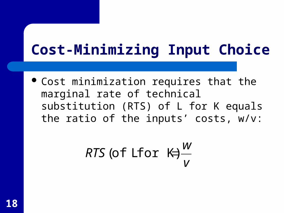
Cost-Minimizing Input Choice
Cost minimization requires that the marginal rate of technical substitution (RTS) of L for K equals the ratio of the inputs’ costs, w/v:
v
wRTS for K) Lof(
19
Graphic Presentation
The isoquant q1 shows all combinations of K and L that are required to produce q1.
The slope of total costs, TC = wL + vK, is -w/v.
Lines of equal cost will have the same slope so they will be parallel.
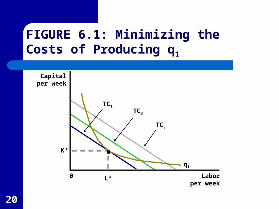
Three equal total costs lines, labeled TC1, TC2, and TC3 are shown in Figure 6.1.
20
Capitalper week
TC1
TC2
TC3
q1
K*
Laborper week
L*0
FIGURE 6.1: Minimizing the Costs of Producing q1
21
Graphic Presentation
The minimum total cost of producing q1 is TC1 (since it is closest to the origin).
The cost-minimizing input combination is L*, K* which occurs where the total cost curve is tangent to the isoquant.
At the point of tangency, the rate at which the firm can technically substitute L for K (the RTS) equals the market rate (w/v).
22
An Alternative Interpretation
.
,
.K)for L of(
v
MP
w
MP
v
w
MP
MPRTS
MP
MPRTS
KL
K
L
K
L
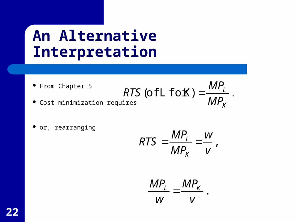
From Chapter 5
Cost minimization requires
or, rearranging
23
The Firm’s Expansion Path
A similar analysis could be performed for any output level (q).
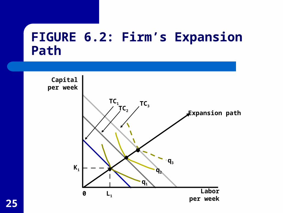
If input costs (w and v) remain constant, various cost-minimizing choices can be traces out as shown in Figure 6.2.
For example, output level q1 is produced using K1, L1, and other cost-minimizing points are shown by the tangency between the total cost lines and the isoquants.
24
The Firm’s Expansion Path
The firm’s expansion path is the set of cost-minimizing input combinations a firm will choose to produce various levels of output (when the prices of inputs are held constant).
Although in Figure 6.2, the expansion path is a straight line, that is not necessarily the case.
25
Capitalper week
TC1 TC3TC2 Expansion path
q1
q2
q3
K1
Laborper week
L10
FIGURE 6.2: Firm’s Expansion Path
26
Cost Curves
A firm’s expansion path shows how minimum-cost input use increases when the level of output expands.
With this it is possible to develop the relationship between output levels and total input costs.
These cost curves are fundamental to the theory of supply.
27
Cost Curves
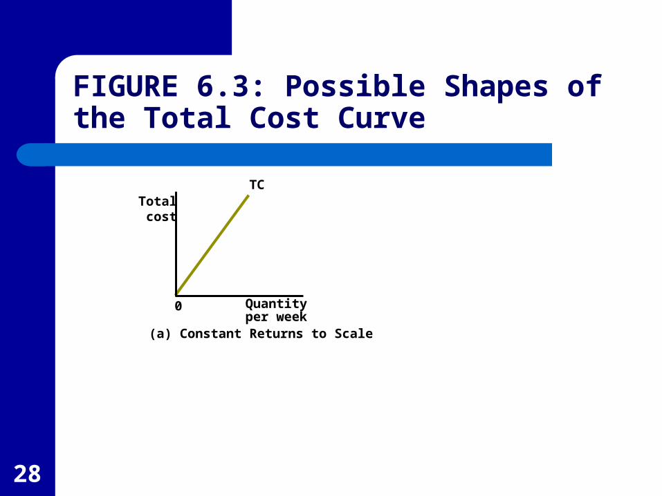
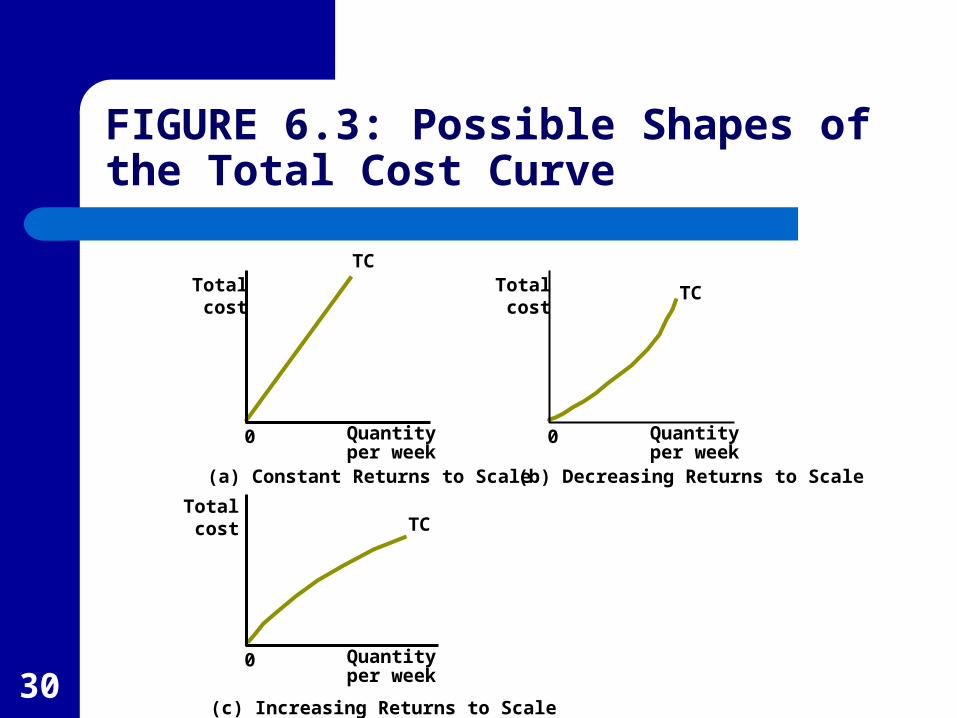
Figure 6.3 shows four possible shapes for cost curves.
In Panel a, output and required input use is proportional which means doubling of output requires doubling of inputs. This is the case when the production function exhibits constant returns to scale.
28
Totalcost
TC
Quantityper week
(a) Constant Returns to Scale
0
FIGURE 6.3: Possible Shapes of the Total Cost Curve
29
Cost Curves
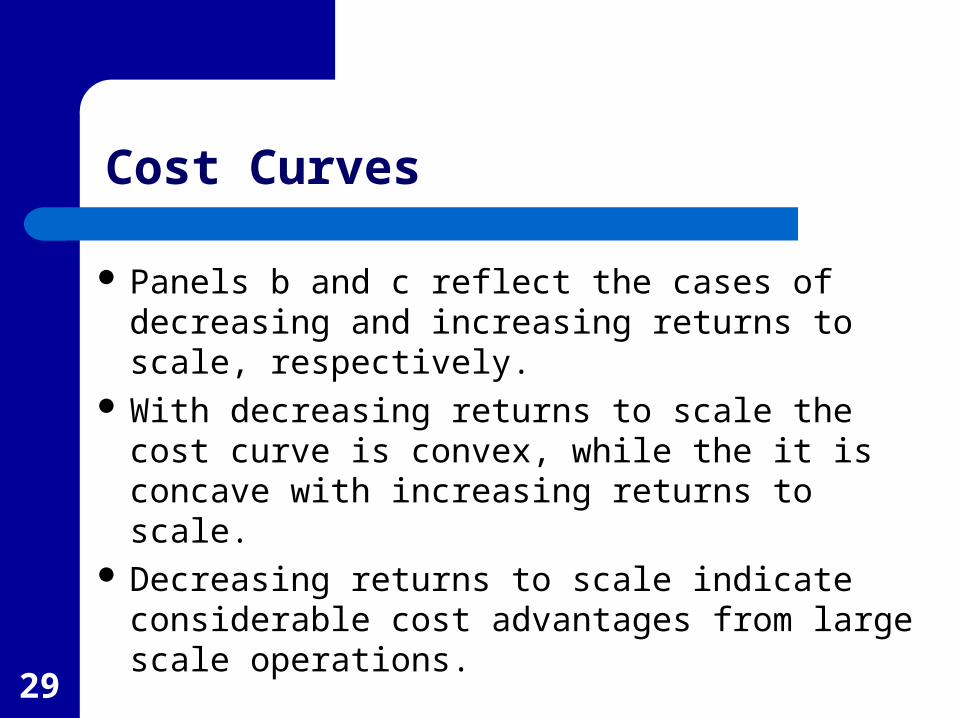
Panels b and c reflect the cases of decreasing and increasing returns to scale, respectively.
With decreasing returns to scale the cost curve is convex, while the it is concave with increasing returns to scale.
Decreasing returns to scale indicate considerable cost advantages from large scale operations.
30
Totalcost
TC
Quantityper week
(a) Constant Returns to Scale
0
Totalcost
TC
Quantityper week
(b) Decreasing Returns to Scale
0
Totalcost TC
Quantityper week
(c) Increasing Returns to Scale
0
FIGURE 6.3: Possible Shapes of the Total Cost Curve
31
Cost Curves
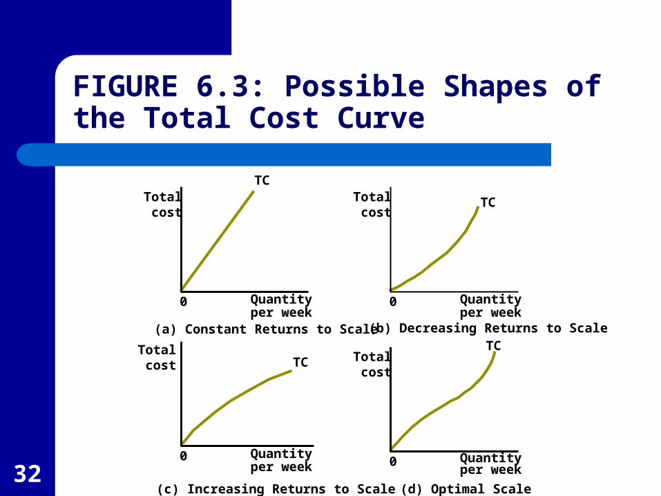
Panel d reflects the case where there are increasing returns to scale followed by decreasing returns to scale.
This might arise because internal co-ordination and control by managers is initially underutilized, but becomes more difficult at high levels of output.
This suggests an optimal scale of output.
32
Totalcost
TC
Quantityper week
(a) Constant Returns to Scale
0
Totalcost
TC
Quantityper week
(b) Decreasing Returns to Scale
0
Totalcost TC
Quantityper week
(c) Increasing Returns to Scale
0
Totalcost
TC
Quantityper week
(d) Optimal Scale
0
FIGURE 6.3: Possible Shapes of the Total Cost Curve
33
Average Costs
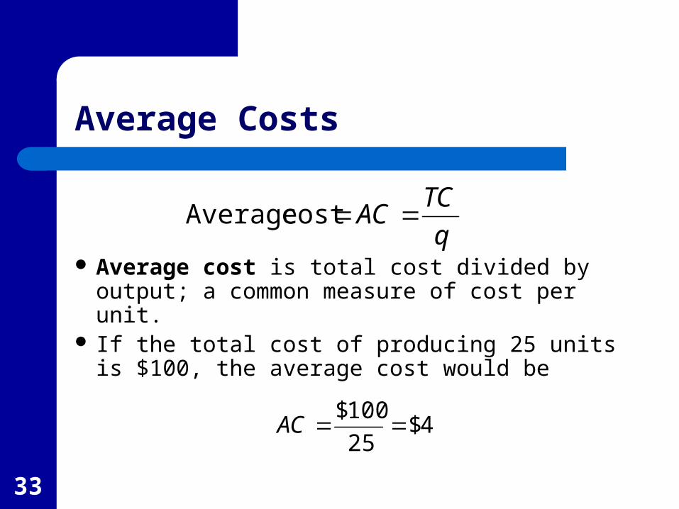
Average cost is total cost divided by output; a common measure of cost per unit.
If the total cost of producing 25 units is $100, the average cost would be
q
TCAC cost Average
4$25
100$AC
34
Marginal Cost
The additional cost of producing one more unit of output is marginal cost.
If the cost of producing 24 units is $98 and the cost of producing 25 units is $100, the marginal cost of the 25th unit is $2.
q in Change
TC in Changecost Marginal MC
35
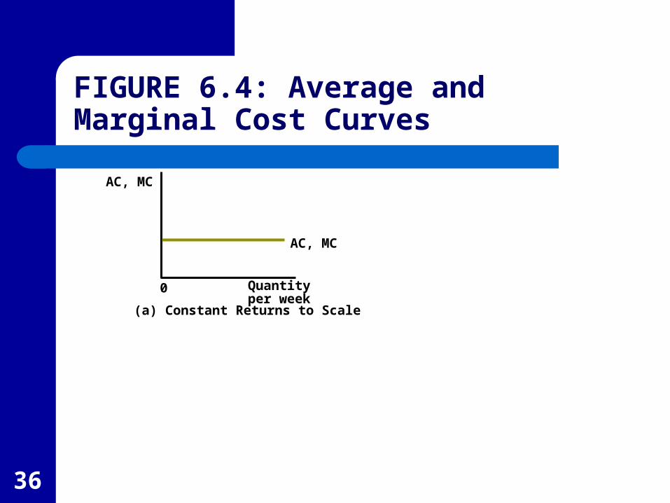
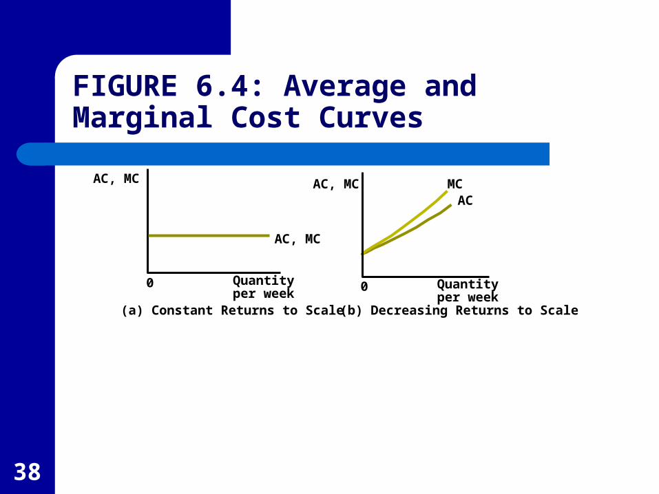
Marginal Cost Curves
Marginal costs are reflected by the slope of the total cost curve.
The constant returns to scale total cost curve shown in Panel a of Figure 6.3 has a constant slope, so the marginal cost is constant as shown by the horizontal marginal cost curve in Panel a of Figure 6.4.
36
AC, MC
AC, MC
Quantityper week
(a) Constant Returns to Scale
0
FIGURE 6.4: Average and Marginal Cost Curves
37
Marginal Cost Curves
With decreasing returns to scale, the total cost curve is convex (Panel b of Figure 6.3).
This means that marginal costs are increasing which is shown by the positively sloped marginal cost curve in Panel b of Figure 6.4.
38
AC, MC
AC, MC
Quantityper week
(a) Constant Returns to Scale
0
AC, MCAC
MC
Quantityper week
(b) Decreasing Returns to Scale
0
FIGURE 6.4: Average and Marginal Cost Curves
39
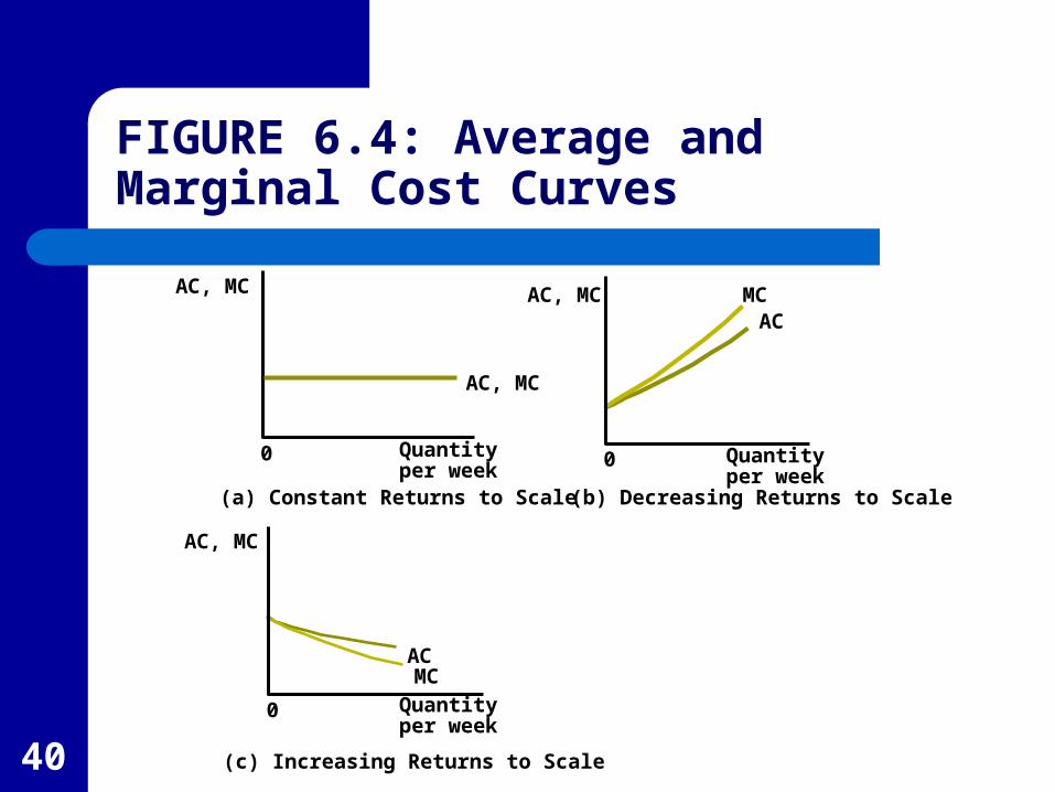
Marginal Cost Curves
Increasing returns to scale results in a concave total cost curve (Panel c of Figure 6.3).
This causes the marginal costs to decrease as output increases as shown in the negatively sloped marginal cost curve in Panel c of Figure 6.4.
40
AC, MC
AC, MC
Quantityper week
(a) Constant Returns to Scale
0
AC, MCAC
AC
MC
MC
Quantityper week
(b) Decreasing Returns to Scale
0
AC, MC
Quantityper week
(c) Increasing Returns to Scale
0
FIGURE 6.4: Average and Marginal Cost Curves
41
Marginal Cost Curves
When the total cost curve is first concave followed by convex as shown in Panel d of Figure 6.3, marginal costs initially decrease but eventually increase.
Thus, the marginal cost curve is first negatively sloped followed by a positively sloped curve as shown in Panel d of Figure 6.4.

42
AC, MC
AC, MC
Quantityper week
(a) Constant Returns to Scale
0
AC, MCAC
AC
AC
MC
MC
MC
Quantityper week
(b) Decreasing Returns to Scale
0
AC, MC
Quantityper week
(c) Increasing Returns to Scale
0
AC, MC
Quantityper week
(d) Optimal Scale
0 q*
FIGURE 6.4: Average and Marginal Cost Curves
43
Average Cost Curves
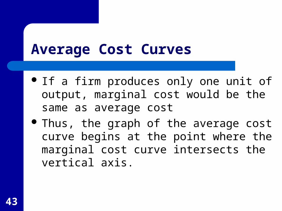
If a firm produces only one unit of output, marginal cost would be the same as average cost
Thus, the graph of the average cost curve begins at the point where the marginal cost curve intersects the vertical axis.
44
Average Cost Curves
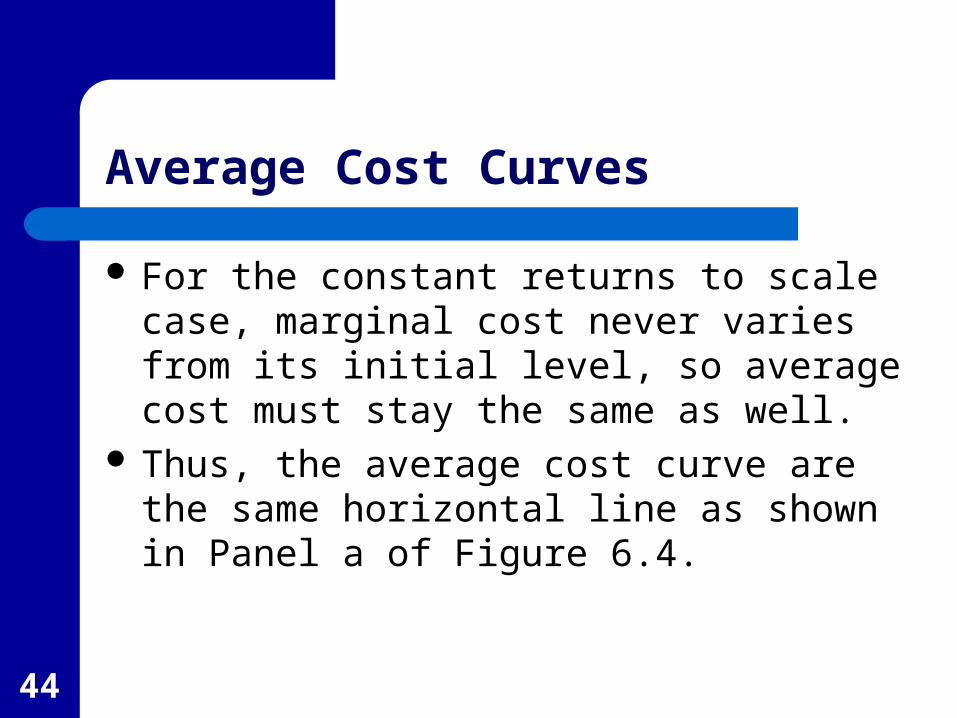
For the constant returns to scale case, marginal cost never varies from its initial level, so average cost must stay the same as well.
Thus, the average cost curve are the same horizontal line as shown in Panel a of Figure 6.4.
45
Average Cost Curves
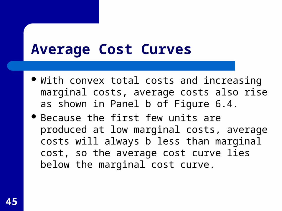
With convex total costs and increasing marginal costs, average costs also rise as shown in Panel b of Figure 6.4.
Because the first few units are produced at low marginal costs, average costs will always b less than marginal cost, so the average cost curve lies below the marginal cost curve.
46
Average Cost Curves
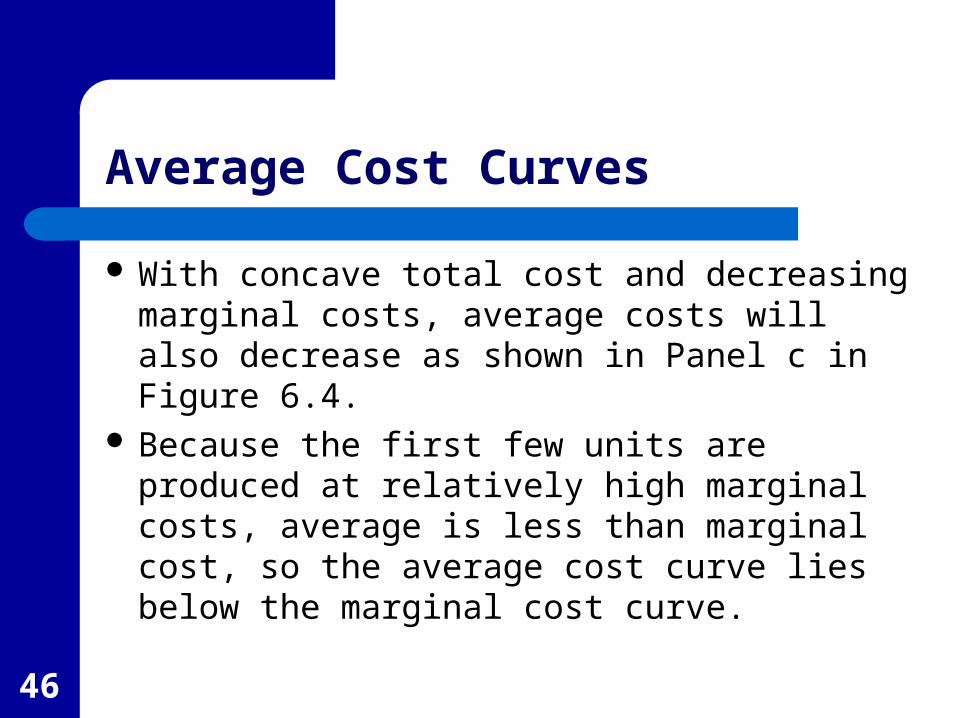
With concave total cost and decreasing marginal costs, average costs will also decrease as shown in Panel c in Figure 6.4.
Because the first few units are produced at relatively high marginal costs, average is less than marginal cost, so the average cost curve lies below the marginal cost curve.
47
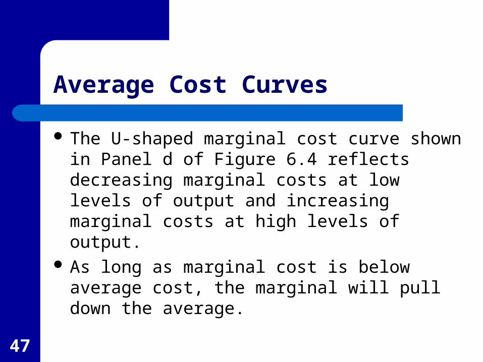
Average Cost Curves
The U-shaped marginal cost curve shown in Panel d of Figure 6.4 reflects decreasing marginal costs at low levels of output and increasing marginal costs at high levels of output.
As long as marginal cost is below average cost, the marginal will pull down the average.
48
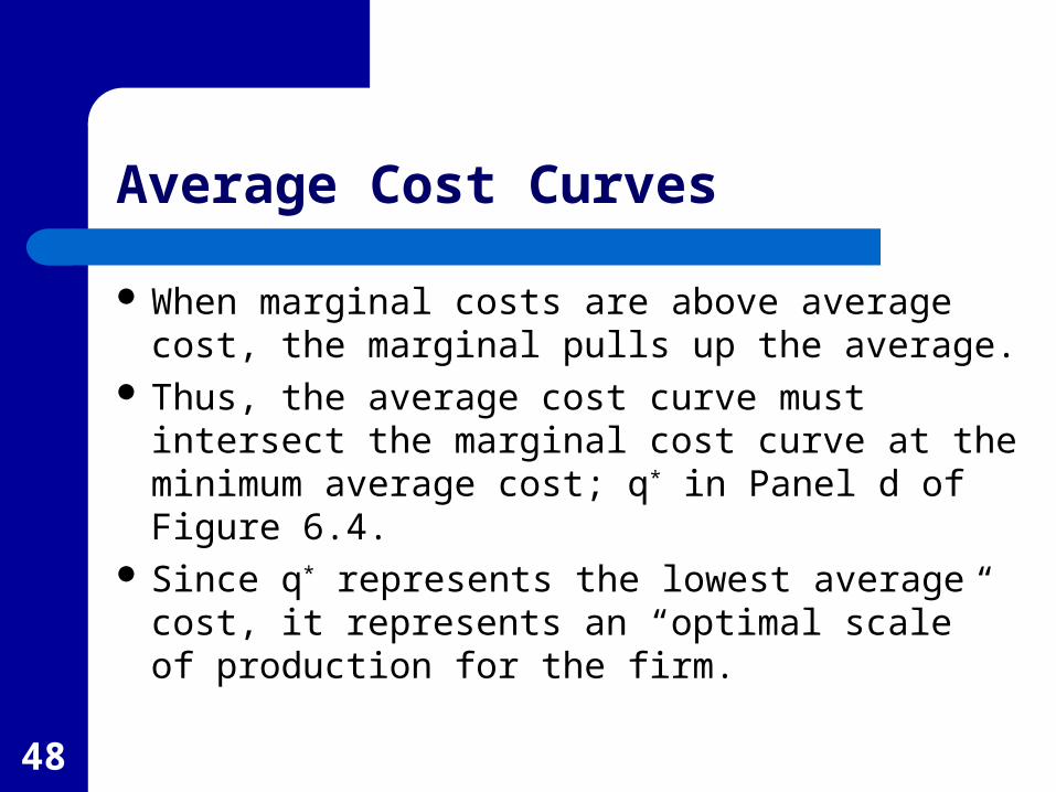
Average Cost Curves
When marginal costs are above average cost, the marginal pulls up the average.
Thus, the average cost curve must intersect the marginal cost curve at the minimum average cost; q* in Panel d of Figure 6.4.
Since q* represents the lowest average cost, it represents an “optimal scale” of production for the firm.
49
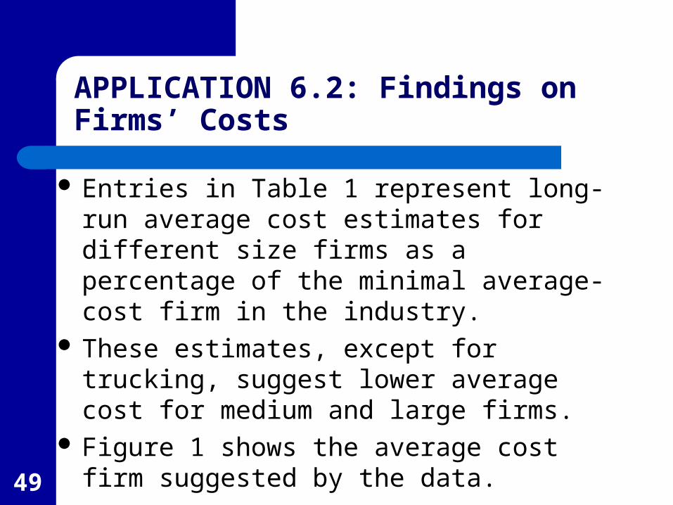
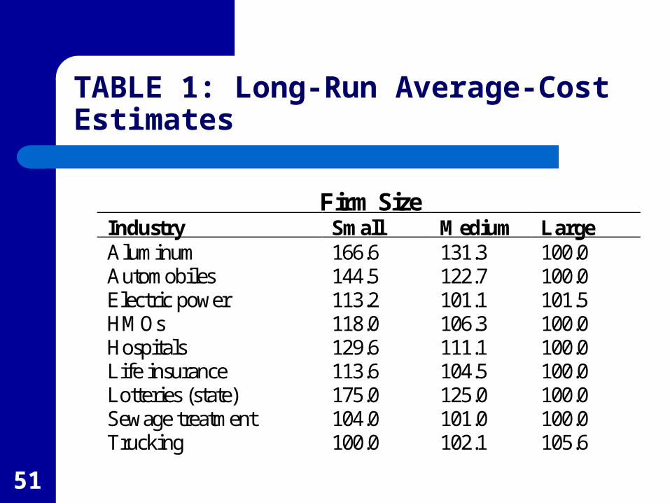
APPLICATION 6.2: Findings on Firms’ Costs
Entries in Table 1 represent long-run average cost estimates for different size firms as a percentage of the minimal average-cost firm in the industry.
These estimates, except for trucking, suggest lower average cost for medium and large firms.
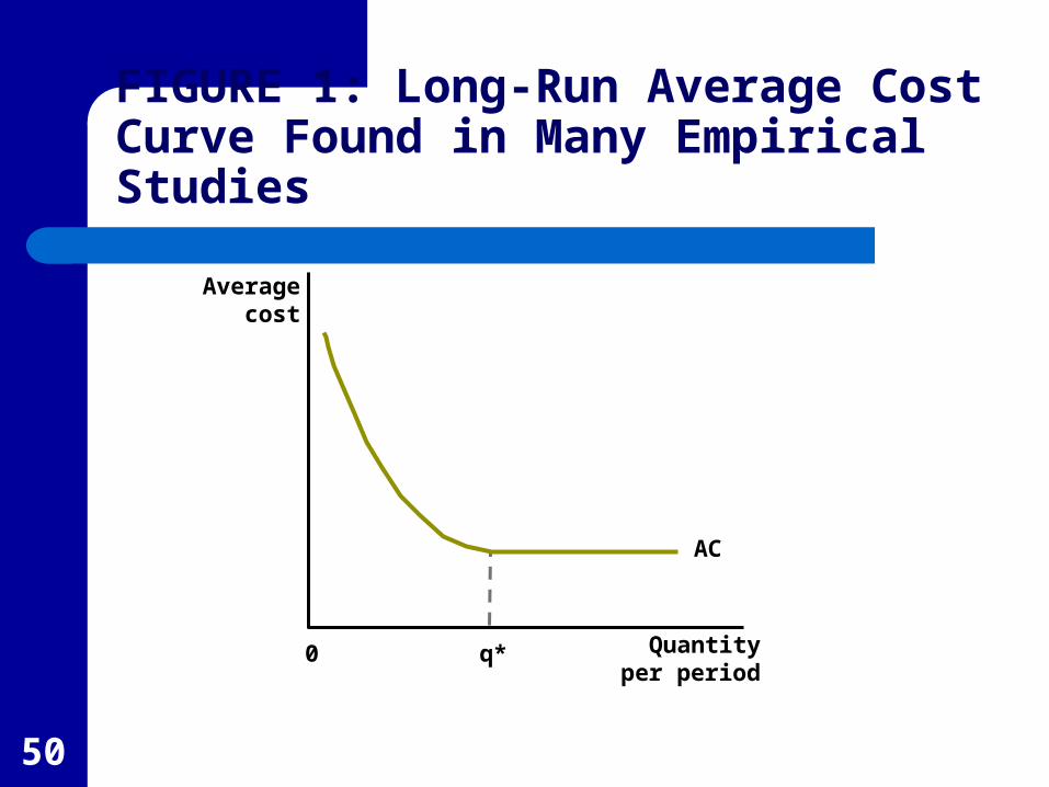
Figure 1 shows the average cost firm suggested by the data.
50
Averagecost
Quantityper period
0 q*
AC
FIGURE 1: Long-Run Average Cost Curve Found in Many Empirical Studies
51
TABLE 1: Long-Run Average-Cost Estimates
Firm Size Industry Small Medium Large Aluminum 166.6 131.3 100.0 Automobiles 144.5 122.7 100.0 Electric power 113.2 101.1 101.5 HMOs 118.0 106.3 100.0 Hospitals 129.6 111.1 100.0 Life insurance 113.6 104.5 100.0 Lotteries (state) 175.0 125.0 100.0 Sewage treatment 104.0 101.0 100.0 Trucking 100.0 102.1 105.6
52
APPLICATION 6.3: Airlines’ Costs
Costs for airlines have been of interest to economists because of recent changes such as deregulation, bankruptcy, and mergers.
Two general findings:– Costs seem to differ substantially among U.S. firms.– Costs for U.S. airlines appear to be significantly
lower than for airlines in other countries.
53
Reasons for Differences among U.S. Firms
Airlines that fly longer average distances or operate a greater number of flights over a given network tend to have lower costs.– Firms can spread the fixed costs associated with
terminals, maintenance facilities, and reservation systems over a larger output volume.
54
Reasons for Differences among U.S. Firms
Firms that operate older fleets or that operate fleets with many different types of planes tend to have higher maintenance and fuel costs.
Wage costs, especially for pilots, also differ significantly among the airlines.
55
International Airline Regulation and Costs
Many foreign carriers’ have not adopted the “hub and spoke” system which appears to be more efficient.
Foreign firms are subject to more regulation.– This situation appears to be changing. For
example, Australia ended rigid controls and costs fell by 15 to 20 percent.
56
Distinction between the Short Run and the Long Run
The short run is the period of time in which a firm must consider some inputs to be absolutely fixed in making its decisions.
The long run is the period of time in which a firm may consider all of its inputs to be variable in making its decisions.
57
Holding Capital Input Constant
For the following, the capital input is assumed to be held constant at a level of K1, so that, with only two inputs, labor is the only input the firm can vary.
As examined in Chapter 5, this implies diminishing marginal productivity to labor.
58
Types of Short-Run Costs
Fixed costs; costs associated with inputs that are fixed in the short run.
Variable costs; costs associated with inputs that can be varied in the short run.
59
Input Inflexibility and Cost Minimization
Since capital is fixed, short-run costs are not the minimal costs of producing variable output levels.
Assume the firm has fixed capital of K1 as shown in Figure 6.5.
To produce q0 of output, the firm must use L1 units of labor, with similar situations for q1, L1, and q2, L2.
60
Capitalper week
STC0 STC2STC1
q1
q2
q0
K1
Laborper week
L0 L1 L20
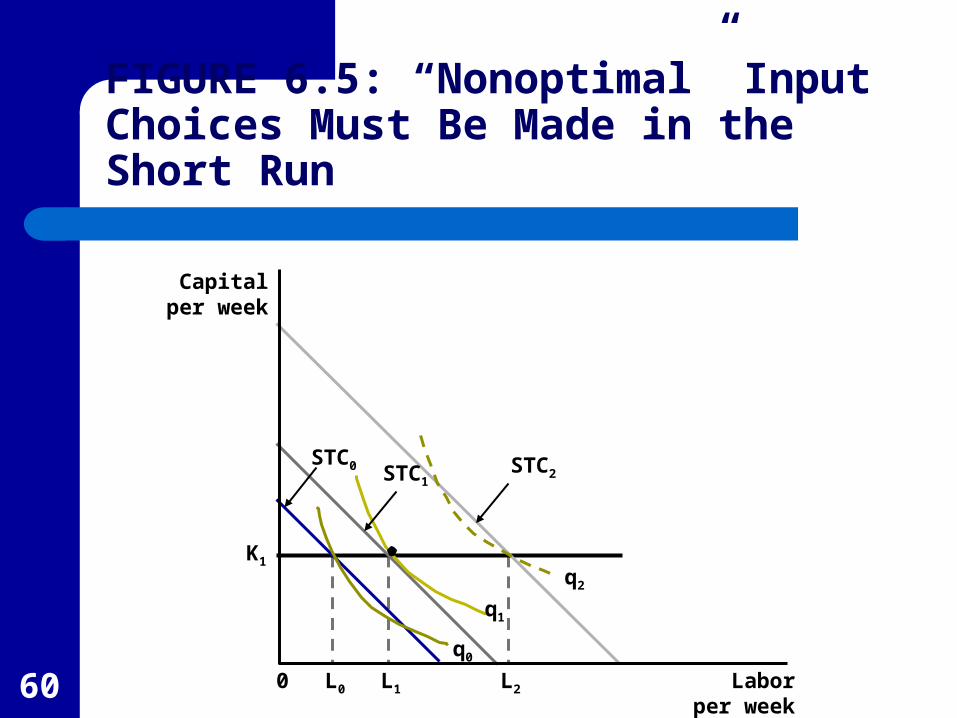
FIGURE 6.5: “Nonoptimal” Input Choices Must Be Made in the Short Run
61
Input Inflexibility and Cost Minimization
The cost of output produced is minimized where the RTS equals the ratio of prices, which only occurs at q1, L1.
Q0 could be produce at less cost if less capital than K1 and more labor than L0 were used.
Q2 could be produced at less cost if more capital than K1 and less labor than L2 were used.
62
Per-Unit Short-Run Cost Curves
q in Change
STC in Changecost marginal run-Short
and
cost average run-Short
SMC
q
STCSAC
63
Per-Unit Short-Run Cost Curves
Having capital fixed in the short run yields a total cost curve that has both concave and convex sections, the resulting short-run average and marginal cost relationships will also be U-shaped.
When SMC < SAC, average cost is falling, but when SMC > SAC average cost increase.
64
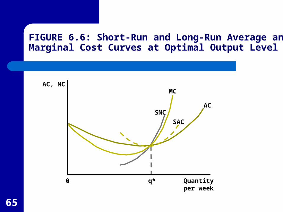
Relationship between Short-Run and Long-Run per-Unit Cost Curves
Figure 6.6 shows all cost relationships for a firm that has U-shaped long-run average and marginal cost curves.
At output level q* long-run average costs are minimized and MC = AC.
Associated with q* is a certain level of capital, K*.
65
SMC
MC
SAC
AC
AC, MC
Quantityper week
0 q*
FIGURE 6.6: Short-Run and Long-Run Average and Marginal Cost Curves at Optimal Output Level
66
Relationship between Short-Run and Long-Run per-Unit Cost Curves
In the short-run, when the firm using K* units of capital produces q*, short-run and long-run total costs are equal.
In addition, as shown in Figure 6.6 AC = MC = SAC(K*) = SMC(K*).
For output above q* short-run costs are higher than long-run costs. The higher per-unit costs reflect the facts that K is fixed.
67
APPLICATION 6.4: Can We Do Anything About Traffic Snarls?
For any traffic facility (road, bridge, tunnel, and so forth), output is measured in number of vehicles per hour.
Capital costs are largely fixed, as depreciation occurs regardless of the level of traffic.
Variable costs consist primarily of motorists’ time.
68
APPLICATION 6.4: Can We Do Anything About Traffic Snarls?
Studies, based on people’s willingness to spend time commuting, indicate travel time “costs” about $8 per hour.
The marginal cost of producing “one more trip” is the overall increase in travel time experienced by all motorists when one more vehicle uses a traffic facility.
69
APPLICATION 6.4: Can We Do Anything About Traffic Snarls?
The high costs associated with adding an extra automobile to an already crowded facility are not directly experienced by the motorist driving the car, because these costs are imposed on other motorists.
This divergence between the private costs and the total social costs leads to motorists opting for overutilizeing traffic facilities.

70
Congestion Tolls
The standard economists answer to this problem is to adopt taxes that bring social and private marginal costs into agreement.
This implies the adoption of highway, bridge, or tunnel tolls, that accurately reflect social costs.
Since these costs vary by time of day, tolls should also vary over the day.

71
Toll-Collecting Technology
This approach was previously not feasible since collection booths for tolls would add more to the congestion that in aiding to the solving of the problem.
However, the development of low-cost electronic toll collection techniques, now make it possible using cards with pre-coded computer chips.

72
Shifts in Cost Curves
Any change in economic conditions that affects the expansion path will also affect the shape and position of the firm’s cost curves.
Three sources of such change are:– change in input prices– technological innovations, and– economies of scope.

73
Changes in Input Prices
A change in the price of an input will tilt the firm’s total cost lines and alter its expansion path.
For example, a rise in wage rates will cause firms to use more capital (to the extent allowed by the technology) and the entire expansion path will rotate toward the capital axis.
74
Changes in Input Prices
Generally, all cost curves will shift upward with the extent of the shift depending upon how important labor is in production and how successful the firm is in substituting other inputs for labor.– With important labor and poor substitution
possibilities, a significant increase in costs will result.
75
Technological Innovation
Because technological advances alter a firm’s production function, isoquant maps as well as the firm’s expansion path will shift when technology changes.
Unbiased improvements would shift isoquants toward the origin enabeling firms to produce the same level of output with less of all inputs.
76
Technological Innovation
Technological change that is biased toward the use of one input will alter isoquant maps, shift expansion paths, and affect the shape and location of cost curves.– For example, if workers became more skilled, this
would save only on labor input.

77
Economies of Scope
Economies of scope is the reduction in the costs of one product of a multiproduct firm when the output of another product is increased.– For example, when hospitals do many surgeries of
one type, it may have cost advantages in doing other types because of the similarities in equipment and operating personnel used.
78
APPLICATION 6.5: Economies of Scope in Banks and Hospitals
Banks and hospitals are both complex types of firms that produce many different products.
Recently, a large number of mergers has occurred in both of these industries.
One of the primary reasons for expected the lower costs associated with these mergers is that the mergers make it possible for firms to have a broader array of products.
79
APPLICATION 6.5: Economies of Scope in Banks and Hospitals
If economies of scope are important, the additional production after mergers, may cause the costs of these firms’ traditional business lines to be lower.
Banks represent an industry where for-profit firms dominate whereas hospitals are more commonly regarded as nonprofit firms.
80
APPLICATION 6.5: Economies of Scope in Banks and Hospitals
Banks are financial intermediaries. Economies of scope can reduce banks’ costs if the
costs associated with any one particular financial product fall when the bank offers other products.
The possibility of economies of scope has played an important role in the evolution of banking regulations (e.g. Glass-Steagall Acts in the U.S. and the more flexible merger guidelines adopted by the European Community.)
81
APPLICATION 6.5: Economies of Scope in Banks and Hospitals
Although most hospitals are not intended to earn economic profits, they still face revenue constraints that push them toward cost-minimization.
Economies of scope arise in a variety of hospital activities
– Facilities for surgical operations tend to have lower costs the wider the variety of operations that are done
– The provision of of outpatient services, running intensive care units, and establishing hospital owned pharmacies also lead to economies of scope.
82
A Numerical Example
Assume Hamburger Heaven (HH) can hire workers at $5 per hour and it rents all of its grills for $5 per hour.
Total costs for HH during one hour are TC = 5K + 5L
where K and L are the number of grills and the number of workers hired during that hour, respectively.
83
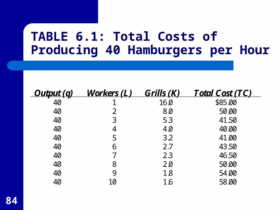
A Numerical Example
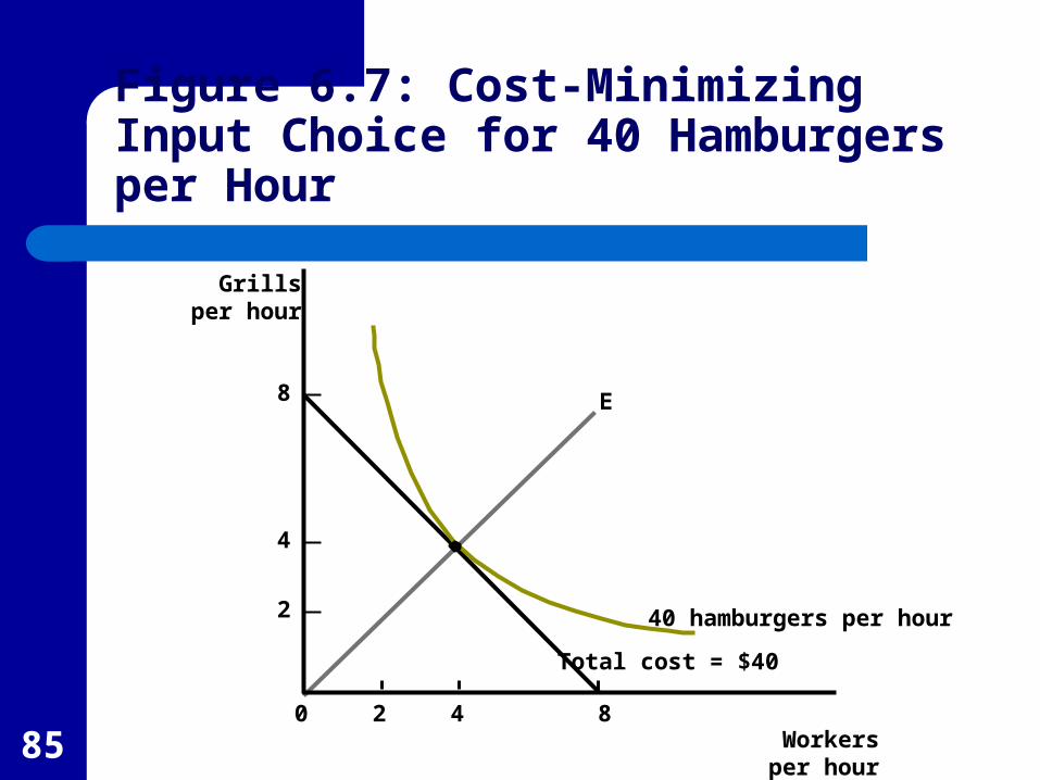
Suppose HH wishes to produce 40 hamburgers per hour.
Table 6.1 repeats the various ways HH can produce 40 hamburgers per hour.– This shows that total costs are minimized when
K = L = 4.
Figure 6.10 shows the cost-minimizing tangency.
84
TABLE 6.1: Total Costs of Producing 40 Hamburgers per Hour
Output (q) Workers (L) Grills (K) Total Cost (TC) 40 1 16.0 $85.00 40 2 8.0 50.00 40 3 5.3 41.50 40 4 4.0 40.00 40 5 3.2 41.00 40 6 2.7 43.50 40 7 2.3 46.50 40 8 2.0 50.00 40 9 1.8 54.00 40 10 1.6 58.00
85
Grillsper hour
2
8
4
Workersper hour
40 hamburgers per hour
E
Total cost = $40
2 4 80
Figure 6.7: Cost-Minimizing Input Choice for 40 Hamburgers per Hour
86
Long-Run cost Curves
HH’s production function is constant returns to scale so
As long as w = v = $5, all of the cost minimizing tangencies will resemble the one shown in Figure 6.10 and long-run cost minimization will require K = L.
87
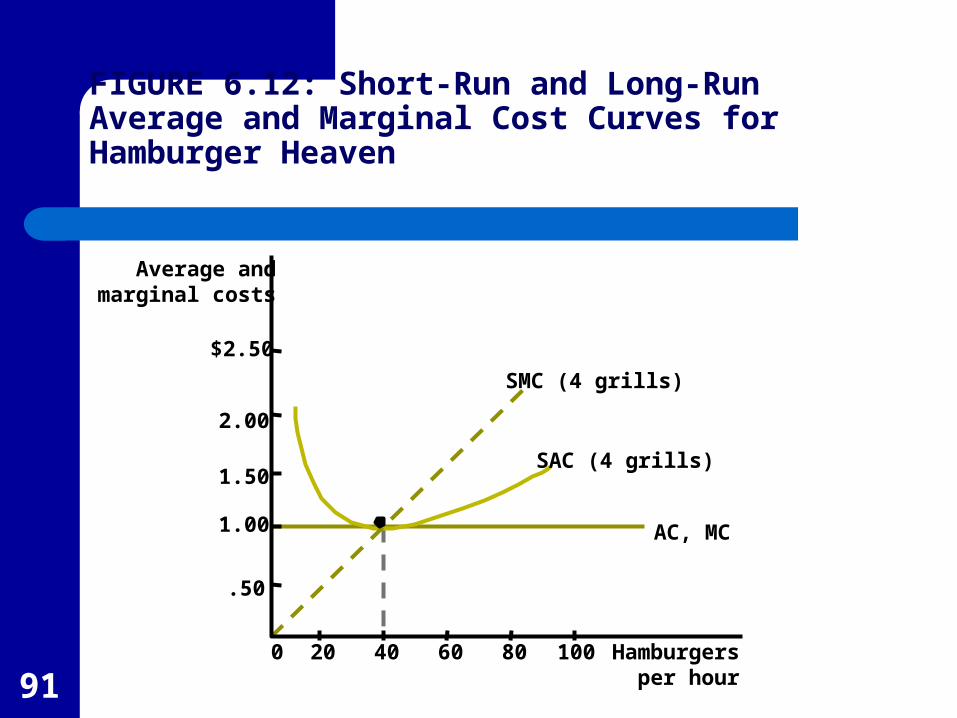
Long-Run cost Curves
This situation, resulting from constant returns to scale, is shown in Figure 6.8.
HH’s long-run total cost function is a straight line through the origin as shown in Panel a.
Its long-run average and marginal costs are constant at $1 per burger as shown in Panel b.
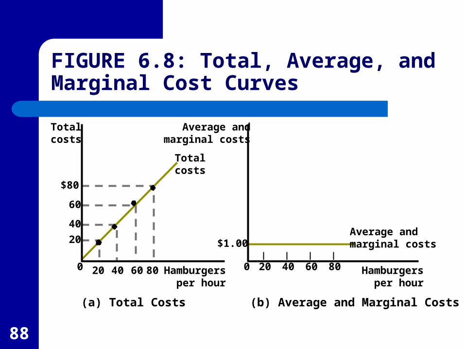
88
Totalcosts
20
60
$80
40
Totalcosts
40 6020 80
(a) Total Costs
0
Average andmarginal costs
$1.00
Hamburgersper hour
40 6020 80
(b) Average and Marginal Costs
0
FIGURE 6.8: Total, Average, and Marginal Cost Curves
Average andmarginal costs
Hamburgersper hour
89
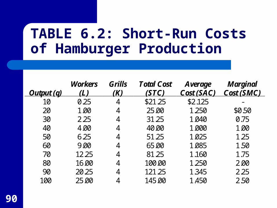
Short-Run Costs
Table 6.2 repeats the labor input required to produce various output levels holding grills fixed at 4.
Diminishing marginal productivity of labor causes costs to rise rapidly as output expands.
Figure 6.9 shows the short-run average and marginal costs curves.
90
TABLE 6.2: Short-Run Costs of Hamburger Production
Output (q) Workers
(L) Grills (K)
Total Cost (STC)
Average Cost (SAC)
Marginal Cost (SMC)
10 0.25 4 $21.25 $2.125 - 20 1.00 4 25.00 1.250 $0.50 30 2.25 4 31.25 1.040 0.75 40 4.00 4 40.00 1.000 1.00 50 6.25 4 51.25 1.025 1.25 60 9.00 4 65.00 1.085 1.50 70 12.25 4 81.25 1.160 1.75 80 16.00 4 100.00 1.250 2.00 90 20.25 4 121.25 1.345 2.25 100 25.00 4 145.00 1.450 2.50
91
Average andmarginal costs
.50
1.00
$2.50
2.00
1.50
Hamburgersper hour
SMC (4 grills)
SAC (4 grills)
AC, MC
4020 60 80 1000
FIGURE 6.12: Short-Run and Long-Run Average and Marginal Cost Curves for Hamburger Heaven