Chapter 6 Discounting Future Benefits and Costs D - epa.gov · Chapter 6 . Discounting Future ... the broad society-as-a-whole point of view that is embodied in benefit-cost analysis

Guidelines for Preparing Economic Analyses | December 2010 6-1

Chapter 6

Discounting Future Benefits and Costs

Discounting renders benefits and costs that occur in different time periods comparable by expressing their values in present terms. In practice, it is accomplished by multiplying the changes in future consumption (broadly defined, including market and non-market goods and services) caused by a policy by a discount factor. At a summary level, discounting reflects

that people prefer consumption today to future consumption, and that invested capital is productive and provides greater consumption in the future. Properly applied, discounting can tell us how much future benefits and costs are worth today.

Social discounting, the type of discounting discussed in this chapter, is discounting from the broad society-as-a-whole point of view that is embodied in benefit-cost analysis (BCA). Private discounting, on the other hand, is discounting from the specific, limited perspective of private individuals or firms. Implementing this distinction can be complex but it is an important distinction to maintain because using a given private discount rate instead of a social discount rate can bias results as part of a BCA.

This chapter addresses discounting over the relatively short term, what has become known as intragenerational discounting, as well as discounting over much longer time horizons, or intergenerational discounting. Intragenerational, or conventional, discounting applies to contexts that may have decades-long time frames, but do not explicitly confront impacts on unborn generations that may be beyond the private planning horizon of the current ones. Intergenerational discounting, by contrast, addresses extremely long time horizons and the impacts and preferences of generations to come. To some extent this distinction is a convenience as there is no discrete point at which one moves from one context to another. However, the relative importance of various issues can change as the time horizon lengthens.

Several sensitive issues surround the choice of discount rate. This chapter attempts to address those most important for applied policy analysis. In addition to the sensitivity of the discount rate to the choice of discounting approach, a topic discussed throughout this chapter, these issues include: the distinction and potential confounding of efficiency and equity considerations (Section 6.3.2.1); the difference between consumption and utility discount rates (Sections 6.2.2.2 and 6.3.1); “prescriptive” vs. “descriptive” approaches to discount rate selection (Section 6.3.1); and uncertainty about future economic growth and other conditions (Sections 6.3.2.1 and 6.3.2.2).

6-2 Guidelines for Preparing Economic Analyses | December 2010

Chapter 6 Discounting Future Benefits and Costs

6.1 The Mechanics of Summarizing Present and Future Costs and BenefitsDiscounting reflects: (1) the amount of time between the present and the point at which these changes occur; (2) the rate at which consumption is expected to change over time in the absence of the policy; (3) the rate at which the marginal value of consumption diminishes with increased consumption; and (4) the rate at which the future utility from consumption is discounted with time. Changes in these components or uncertainty about them can lead to a discount rate that changes over time, but for many analyses it may be sufficient to apply a fixed discount rate or rates without explicit consideration of the constituent components or uncertainty.1

There are several methods for discounting future values to the present, the most common of which involve estimating net present values and annualized values. An alternative is to estimate a net future value.

6.1.1 Net Present Value (NPV)The NPV of a projected stream of current and future benefits and costs relative to the analytic baseline is estimated by multiplying the benefits and costs in each year by a time-dependent weight, or discount factor, d, and adding all of the weighted values as shown in the following equation:

NPV = NB0 + d1NB1 + d2NB2 + ... + dn–1NBn–1 + dnNBn (1)

where NBt is the net difference between benefits and costs (Bt - Ct) that accrue at the end of period t. The discounting weights, dt, are given by:

dt = (1 1 + r)t (2)

where r is the discount rate. The final period of the policy’s future effects is designated as time n.

1 Note that accounting for changes in these components through discounting is distinct from accounting for inflation, although observed market rates reflect expected inflation. Both values (i.e., benefits and costs) and the discount rate should be adjusted for inflation; therefore most of the discussion in this chapter focuses on real discount rates and values.

The NPV can be estimated using real or nominal benefits, costs, and discount rates. The analyst can estimate the present value of costs and benefits separately and then compare them to arrive at net present value.

It is important that the same discount rate be used for both benefits and costs because nearly any policy can be justified by choosing a sufficiently low discount rate for benefits, by choosing sufficiently high discount rates for costs, or by choosing a sufficiently long time horizon. Likewise, making sufficiently extreme opposite choices could result in any policy being rejected.

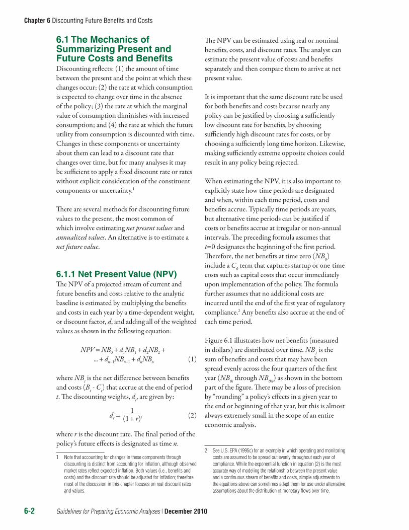
When estimating the NPV, it is also important to explicitly state how time periods are designated and when, within each time period, costs and benefits accrue. Typically time periods are years, but alternative time periods can be justified if costs or benefits accrue at irregular or non-annual intervals. The preceding formula assumes that t=0 designates the beginning of the first period. Therefore, the net benefits at time zero (NB0) include a C0 term that captures startup or one-time costs such as capital costs that occur immediately upon implementation of the policy. The formula further assumes that no additional costs are incurred until the end of the first year of regulatory compliance.2 Any benefits also accrue at the end of each time period.

Figure 6.1 illustrates how net benefits (measured in dollars) are distributed over time. NB1 is the sum of benefits and costs that may have been spread evenly across the four quarters of the first year (NB0i through NB0iv) as shown in the bottom part of the figure. There may be a loss of precision by “rounding” a policy’s effects in a given year to the end or beginning of that year, but this is almost always extremely small in the scope of an entire economic analysis.

2 See U.S. EPA (1995c) for an example in which operating and monitoring costs are assumed to be spread out evenly throughout each year of compliance. While the exponential function in equation (2) is the most accurate way of modeling the relationship between the present value and a continuous stream of benefits and costs, simple adjustments to the equations above can sometimes adapt them for use under alternative assumptions about the distribution of monetary flows over time.



6.1.2 Annualized ValuesAn annualized value is the amount one would have to pay at the end of each time period t so that the sum of all payments in present value terms equals the original stream of values. Producing annualized values of costs and benefits is useful because it converts the time varying stream of values to a constant stream. Comparing annualized costs to annualized benefits is equivalent to comparing the present values of costs and benefits. Costs and benefits each may be annualized separately by using a two-step procedure. While the formulas below illustrate the estimation of annualized costs, the formulas are identical for benefits.3

To annualize costs, the present value of costs is calculated using the above formula for net benefits, except the stream of costs alone, not the net benefits, is used in the calculation. The exact equation for annualizing depends on whether or not there are any costs at time zero (i.e., at t=0).

Annualizing costs when there is no initial cost at t=0 is estimated using the following equation:

AC = PVC * r * (1 + r)n

(1 + r)n – 1 (3)

where

AC = annualized cost accrued at the end of each of n periods;

3 Variants of these formulas may be common in specific contexts. See, for example, the Equivalent Uniform Annual Cost approach in EPA’s Air Pollution Control Cost Manual (U.S. EPA 2002b).

PVC = present value of costs (estimated as in equation 1, above);

r = the discount rate per period; and

n = the duration of the policy.

Annualizing costs when there is initial cost at t=0 is estimated using the following slightly different equation:

AC = PVC * r * (1 + r)n

(1 + r)(n + 1) – 1 (4)

Note that the numerator is the same in both equations. The only difference is the “n+1” term in the denominator.

Annualization of costs is also useful when evaluating non-monetized benefits, such as reductions in emissions or reductions in health risks, when benefits are constant over time. The average cost-effectiveness of a policy or policy option can be calculated by dividing the annualized cost by the annual benefit to produce measures of program effectiveness, such as the cost per ton of emissions avoided.

As mentioned above, the same formulas would apply to estimating annualized benefits.

6.1.3 Net Future ValueInstead of discounting all future values to the present, it is possible to estimate value in some future time period, for example, at the end of the last year of the policy’s effects, n. The net future value is estimated using the following equation:

NFV = d0NB0 + d1NB1 + d2NB2 + ... + dn–1 NBn–1 + NBn (5)

NBt is the net difference between benefits and costs (Bt - Ct) that accrue in year t and the accumulation weights, dt, are given by

dt = (1 + r) (n–t) (6)

Year t 0 1 2 3 4 n...

...$ NB0 NB1 NB2 NB3 NB4 NBn

TIME �

Year t 0 1

$ NB0i NB0ii NB0iii NB0iv

TIME �

Figure 6.1 - Distribution of Net Benefits over Time



where r is the discount rate. It should be noted that the net present value and net future value can be expressed relative to one another:

NPV = (1 1 + r)n (7)

6.1.4 Comparing the MethodsEach of the methods described above uses a discount factor to translate values across time, so the methods are not different ways to determine the benefits and costs of a policy, but rather are different ways to express and compare these costs and benefits in a consistent manner. NPV represents the present value of all costs and benefits, annualization represents the value as spread smoothly through time, and NFV represents their future value. For a given stream of net benefits, the NPV will be lower with higher discount rates, the NFV will be higher with higher discount rates, and the annualized value may be higher or lower depending on the length of time over which the values are annualized. Still, rankings among regulatory alternatives are unchanged across the methods.

Depending on the circumstances, one method might have certain advantages over the others. Discounting to the present to get a NPV is likely to be the most informative procedure when analyzing a policy that requires an immediate investment and offers a stream of highly variable future benefits. However, annualizing the costs of two machines with different service lives might reveal that the one with the higher total cost actually has a lower annual cost because of its longer lifetime.

Annualized values are sensitive to the annualization period; for any given present value the annualized value will be lower the longer the annualization period. Analysts should be careful when comparing annualized values from one analysis to those from another.

The analysis, discussion, and conclusions presented in this chapter apply to all methods of translating costs, benefits, and effects through time, even though the focus is mostly on NPV estimates.

6.1.5 Sensitivity of Present Value Estimates to the Discount Rate The impact of discounting streams of benefits and costs depends on the nature and timing of benefits and costs. The discount rate is not likely to affect the present value of the benefits and costs for those cases in which:

• All effects occur in the same period (discounting may be unnecessary or superfluous because net benefits are positive or negative regardless of the discount rate used);

• Costs and benefits are largely constant over the relevant time frame (discounting costs and benefits will produce the same conclusion as comparing a single year’s costs and benefits); and/or

• Costs and benefits of a policy occur simultaneously and their relative values do not change over time (whether the NPV is positive does not depend on the discount rate, although the discount rate can affect the relative present value if a policy is compared to another policy).

Discounting can, however, substantially affect the NPV of costs and benefits when there is a significant difference in the timing of costs and benefits, such as with policies that require large initial outlays or that have long delays before benefits are realized. Many of EPA’s policies fit these profiles. Text Box 6.1 illustrates a case in which discounting and the choice of the discount rate have a significant impact on a policy’s NPV.

6.1.6 Some Issues in ApplicationThere are several important analytic components that need to be considered when discounting: risk and valuation, placing effects in time, and the length of the analysis.

6.1.6.1 Risk and ValuationThere are two concepts that are often confounded when implementing social discounting, but should be treated separately. The first is the future value of environmental effects, which depends on many factors,



including the availability of substitutes and the level of wealth in the future. The second is the role of risk in valuing benefits and costs. For both of these components, the process of determining their values and then translating the values into present terms are two conceptually distinct procedures. Incorporating the riskiness of future benefits and costs into the social discount rate not only imposes specific and generally unwarranted assumptions, but it can also hide important information from decision makers.

6.1.6.2 Placing Effects in TimePlacing effects properly in time is essential for NPV calculations to characterize efficiency outcomes. Analyses should account for implementation schedules and the resulting changes in emissions or environmental quality, including possible changes in behavior between the announcement of policy and compliance. Additionally, there may be a lag time between changes in environmental quality and a corresponding change in welfare. It is the change in welfare that defines economic value, and not the change in environmental quality itself. Enumerating the time path of welfare changes is essential for proper valuation and BCA.

6.1.6.3 Length of the AnalysisWhile there is little theoretical guidance on the time horizon of economic analyses, a guiding principle is that the time span should be sufficient to capture major welfare effects from policy alternatives. This principle is consistent with the underlying

requirement that BCA reflect the welfare outcomes of those affected by the policy. Another way to view this is to consider that the time horizon, T, of an analysis should be chosen such that:

Σ (Bt – Ct)e–rt ≤ ε , t=T

(8)

where ε is a tolerable estimation error for the NPV of the policy. That is, the time horizon should be long enough that the net benefits for all future years (beyond the time horizon) are expected to be negligible when discounted to the present. In practice, however, it is not always obvious when this will occur because it may be unclear whether or when the policy will be renewed or retired by policy makers, whether or when the policy will become obsolete or “non-binding” due to exogenous technological changes, how long the capital investments or displacements caused by the policy will persist, etc.

As a practical matter, reasonable alternatives for the time span of the analysis may be based on assumptions regarding:

• The expected life of capital investments required by or expected from the policy;

• The point at which benefits and costs reach a steady state;

• Statutory or other requirements for the policy or the analysis; and/or

• The extent to which benefits and costs are separated by generations.

Suppose the benefits of a given program occur 30 years in the future and are valued (in real terms) at $5 billion at that time. The rate at which the $5 billion future benefits is discounted can dramatically alter the economic assessment of the policy: $5 billion 30 years in the future discounted at 1 percent is $3.71 billion, at 3 percent it is worth $2.06 billion, at 7 percent it is worth $657 million, and at 10 percent it is worth only $287 million. In this case, the range of discount rates generates over an order of magnitude of difference in the present value of benefits. Longer time horizons will produce even more dramatic effects on a policy’s NPV (see Section 6.3 on intergenerational discounting). For a given present value of costs, particularly the case where costs are incurred in the present and therefore not affected by the discount rate, it is easy to see that the choice of the discount rate can determine whether this policy is considered, on economic efficiency grounds, to offer society positive or negative net benefits.

Text Box 6.1 - Potential Effects of Discounting



The choice should be explained and well-documented. In no case should the time horizon be arbitrary, and the analysis should highlight the extent to which the sign of net benefits or the relative rankings of policy alternatives are sensitive to the choice of time horizon.

6.2 Background and Rationales for Social Discounting The analytical and ethical foundation of the social discounting literature rests on the traditional test of a “potential” Pareto improvement in social welfare; that is, the trade-off between the gains to those who benefit and the losses to those who bear the costs. This framework casts the consequences of government policies in terms of individuals contemplating changes in their own consumption (broadly defined) over time. Trade-offs (benefits and costs) in this context reflect the preferences of those affected by the policy, and the time dimension of those trade-offs should reflect the intertemporal preferences of those affected. Thus, social discounting should seek to mimic the discounting practices of the affected individuals.

The literature on discounting often uses a variety of terms and frameworks to describe identical or very similar key concepts. General themes throughout this literature are the relationship between consumption rates of interest and the rate of return on private capital, the need for a social rate of time preference for BCA, and the importance of considering the opportunity cost of foregone capital investments.

6.2.1 Consumption Rates of Interest and Private Rates of ReturnIn a perfect capital market with no distortions, the return to savings (the consumption rate of interest) equals the return on private sector investments. Therefore, if the government seeks to value costs and benefits in present day terms in the same way as the affected individuals, it should also discount using this single market rate of interest. In this kind of “first best” world, the market interest rate would be an unambiguous choice for the social discount rate.

Real-world complications, however, make the issue much more complex. Among other things, private sector returns are taxed (often at multiple levels), capital markets are not perfect, and capital investments often involve risks reflected in market interest rates. These factors drive a wedge between the social rate at which consumption can be traded through time (the pre-tax rate of return to private investments) and the rate at which individuals can trade consumption over time (the post-tax consumption rate of interest). Text Box 6.2 illustrates how these rates can differ.

A large body of economic literature analyzes the implications for social discounting of divergences between the social rate of return on private sector investment and the consumption rate of interest. Most of this literature is based on the evaluation of public projects, but many of the insights still apply to regulatory BCA. The dominant approaches in this literature are briefly outlined here. More complete recent reviews can be found in Spackman (2004) and Moore et al. (2004).

Suppose that the market rate of interest, net of inflation, is 5 percent, and that the taxes on capital income amount to 40 percent of the net return. In this case, private investments will yield 5 percent, of which 2 percent is paid in taxes to the government, with individuals receiving the remaining 3 percent. From a social perspective, consumption can be traded from the present to the future at a rate of 5 percent. But individuals effectively trade consumption through time at a rate of 3 percent because they owe taxes on investment earnings. As a result, the consumption rate of interest is 3 percent, which is substantially less than the 5 percent social rate of return on private sector investments (also known as the social opportunity cost of private capital).

Text Box 6.2 - Social Rate and Consumption Rates of Interest



6.2.2 Social Rate of Time PreferenceThe goal of social discounting is to compare benefits and costs that occur at different times based on the rate at which society is willing to make such trade-offs. If costs and benefits can be represented as changes in consumption profiles over time, then discounting should be based on the rate at which society is willing to postpone consumption today for consumption in the future. Thus, the rate at which society is willing to trade current for future consumption, or the social rate of time preference, is the appropriate discounting concept.

Generally a distinction is made between individual rates of time preference and that of society as a whole, which should inform public policy decisions. The individual rate of time preference includes factors such as the probability of death, whereas society can be presumed to have a longer planning horizon. Additionally, individuals routinely are observed to have several different types of savings, each possibly yielding different returns, while simultaneously borrowing at different rates of interest. For these and other reasons, the social rate of time preference is not directly observable and may not equal any particular market rate.

6.2.2.1 Estimating a Social Rate of Time Preference Using Risk-Free AssetsOne common approach to estimating the social rate of time preference is to approximate it from the market rate of interest from long-term, risk-free assets such as government bonds. The rationale behind this approach is that this market rate reflects how individuals discount future consumption, and government should value policy-related consumption changes as individuals do. In other words, the social rate of discount should equal the consumption rate of interest (i.e., an individual’s marginal rate of time preference).

In principle, estimates of the consumption rate of interest could be based on either after-tax lending or borrowing rates. Because individuals may be in different marginal tax brackets, may have different

levels of assets, and may have different opportunities to borrow and invest, the type of interest rate that best reflects marginal time preference will differ among individuals. However, the fact that, on net, individuals generally accumulate assets over their working lives suggests that the after-tax returns on savings instruments generally available to the public will provide a reasonable estimate of the consumption rate of interest.

The historical rate of return, post-tax and after inflation, is a useful measure because it is relatively risk-free, and BCA should address risk elsewhere in the analysis rather than through the interest rate. Also, because these are longer-term instruments, they provide more information on how individuals value future benefits over these kinds of time frames.

6.2.2.2 Estimating a Social Rate of Time Preference Using the ‘Ramsey’ FrameworkA second option is to construct the social rate of time preference in a framework originally developed by Ramsey (1928) to reflect: (1) the value of additional consumption as income changes; and (2) a “pure rate of time preference” that weighs utility in one period directly against utility in a later period. These factors are combined in the equation:

r = g + (9)

where (r) is the market interest rate, the first term is the elasticity of marginal utility () times the consumption growth rate (g), and the second term is pure rate of time preference (). Estimating a social rate of time preference in this framework requires information on each of these arguments, and while the first two of these factors can be derived from data, is unobservable and must be determined.4 A more detailed discussion of the Ramsey equation can be found in Section 6.3: Intergenerational Social Discounting.

4 The Science Advisory Board (SAB) Council defines discounting based on a Ramsey equation as the “demand-side” approach, noting that the value judgments required for the pure social rate of time preference make it an inherently subjective concept (U.S. EPA 2004c).



6.2.3 Social Opportunity Cost of CapitalThe social opportunity cost of capital approach recognizes that funds for government projects, or those required to meet government regulations, have an opportunity cost in terms of foregone investments and therefore future consumption. When a regulation displaces private investments society loses the total pre-tax returns from those foregone investments. In these cases, ignoring such capital displacements and discounting costs and benefits using a consumption rate of interest (the post-tax rate of interest) does not capture the fact that society loses the higher, social (pre-tax) rate of return on foregone investments.

Private capital investments might be displaced if, for example, public projects are financed with government debt or regulated firms cannot pass through capital expenses, and the supply of investment capital is relatively fixed. The resulting demand pressure in the investment market will tend to raise interest rates and squeeze out private investments that would otherwise have been made.5 Applicability of the social opportunity cost of capital depends upon full crowding out of private investments by environmental policies.

The social opportunity cost of capital can be estimated by the pre-tax marginal rate of return on private investments observed in the marketplace. There is some debate as to whether it is best to use only corporate debt, only equity (e.g., returns to stocks) or some combination of the two. In practice, average returns that are likely to be higher than the marginal return, are typically observed, given that firms will make the most profitable investments first; it is not clear how to estimate marginal returns. These rates also reflect risks faced in the private sector, which may not be relevant for public sector evaluation.

5 Another justification for using the social opportunity cost of capital argues that the government should not invest (or compel investment through its policies) in any project that offers a rate of return less than the social rate of return on private investments. While it is true that social welfare will be improved if the government invests in projects that have higher values rather than lower ones, it does not follow that rates of return offered by these alternative projects define the level of the social discount rate. If individuals discount future benefits using the consumption rate of interest, the correct way to describe a project with a rate of return greater than the consumption rate is to say that it offers substantial present value net benefits.

6.2.4 Shadow Price of Capital ApproachUnder the shadow price of capital approach costs are adjusted to reflect the social costs of altered private investments, but discounting for time itself is accomplished using the social rate of time preference that represents how society trades and values consumption over time.6 The adjustment factor is referred to as the “shadow price of capital.”7 Many sources recognize this method as the preferred analytic approach to social discounting for public projects and policies.8

The shadow price, or social value, of private capital is intended to capture the fact that a unit of private capital produces a stream of social returns at a rate greater than that at which individuals discount them. If the social rate of discount is the consumption rate of interest, then the social value of a $1 private sector investment will be greater than $1. The investment produces a rate of return for its owners equal to the post-tax consumption rate of interest, plus a stream of tax revenues (generally considered to be consumption) for the government. Text Box 6.3 illustrates this idea of the shadow price of capital.

If compliance with environmental policies displaces private investments, the shadow price of capital approach suggests first adjusting the project or policy cost upward by the shadow price of capital, and then discounting all costs and benefits using a social rate of discount equal to the social rate of time preference. The most complete frameworks for the shadow price of capital also note that while the costs of regulation might displace private capital, the benefits could encourage additional private sector investments. In principle, a full analysis of shadow price of

6 Because the consumption rate of interest is often used as a proxy for the social rate of time preference, this method is sometimes known as the “consumption rate of interest – shadow price of capital” approach. However, as Lind (1982b) notes, what is really needed is the social rate of time preference, so more general terminology is used. Discounting based on the shadow price of capital is referred to as a “supply side” approach by EPA’s SAB Council (U.S. EPA 2004c).

7 A “shadow price” can be viewed as a good’s opportunity cost, which may not equal the market price. Lind (1982a) remains the seminal source for this approach in the social discounting literature.

8 See OMB Circular A-4 (2003), Freeman (2003), and the report of EPA’s Advisory Council on Clean Air Compliance Analysis (U.S. EPA 2004c).



capital adjustments would treat costs and benefits symmetrically in this sense.

The first step in applying this approach is determining whether private investment flows will be altered by a policy. Next, all of the altered private investment flows (positive and negative) are multiplied by the shadow price of capital to convert them into consumption-equivalent units. All flows of consumption and consumption equivalents are then discounted using the social rate of time preference. A simple illustration of this method applied to the costs of a public project and using the consumption rate of interest is shown in Text Box 6.3.9

9 An alternative approach for addressing the divergence between the higher social rate of return on private investments and lower consumption rate of interest is to set the social discount rate equal to a weighted average of the two. The weights would equal the proportions of project financing that displace private investment and consumption respectively. This approach has enjoyed considerable popularity over the years, but it is technically incorrect and can produce NPV results substantially different from the shadow price of capital approach. (For an example of these potential differences see Spackman 2004.)

6.2.4.1 Estimating the Shadow Price of CapitalThe shadow price of capital approach is data intensive. It requires, among other things, estimates of the social rate of time preference, the social opportunity cost of capital, and estimates of the extent to which regulatory costs displace private investment and benefits stimulate it. While the first two components can be estimated as described earlier, information on regulatory effects on capital formation is more difficult. As a result empirical evidence for the shadow price of capital is less concrete, making the approach difficult to implement.10

Whether or not this adjustment is necessary appears to depend largely on whether the economy in question is assumed to be open or closed, and on the magnitude of the intervention or program

10 Depending on the magnitudes of the various factors, shadow prices from about 1 to infinity can result (Lyon 1990). Lyon (1990) and Moore et al. (2004) contain excellent reviews of how to calculate the shadow price of capital and possible settings for the various parameters that determine its magnitude.

To estimate the shadow price of capital, suppose that the consumption rate of interest is 3 percent, the pre-tax rate of return on private investments is 5 percent, the net-of-tax earnings from these investments are consumed in each period, and the investment exists in perpetuity (amortization payments from the gross returns of the investment are devoted to preserving the value of the capital intact). A $1 private investment under these conditions will produce a stream of private consumption of $.03 per year, and tax revenues of $.02 per year. Discounting the private post-tax stream of consumption at the 3 percent consumption rate of interest yields a present value of $1. Discounting the stream of tax revenues at the same rate yields a present value of about $.67. The social value of this $1 private investment – the shadow price of capital – is thus $1.67, which is substantially greater than the $1 private value that individuals place on it.

To apply this shadow price of capital estimate, we need additional information about debt and tax financing as well as about how investment and consumption are affected. Assume that increases in government debt displace private investments dollar-for-dollar, and that increased taxes reduce individuals’ current consumption also on a one-for-one basis. Finally, assume that the $1 current cost of a public project is financed 75 percent with government debt and 25 percent with current taxes, and that this project produces a benefit 40 years from now that is estimated to be worth $5 in the future.

Using the shadow price of capital approach, first multiply 75 percent of the $1 current cost (which is the amount of displaced private investment) by the shadow price of capital (assume this is the $1.67 figure from above). This yields $1.2525; add to this the $.25 amount by which the project’s costs displace current consumption. The total social cost is therefore $1.5025. This results in a net social present value of about $.03, which is the present value of the future $5 benefit discounted at the 3 percent consumption rate of interest ($1.5328) minus the $1.5025 social cost.

Text Box 6.3 - Estimating and Applying the Shadow Price of Capital



considered relative to the flow of investment capital from abroad.11

Some argue that early analyses implicitly assumed that capital flows into the nation were either nonexistent or very insensitive to interest rates, known as the “closed economy” assumption.12 Some empirical evidence suggests, however, that international capital flows are quite large and are sensitive to interest rate changes. In this case, the supply of investment funds to the U.S. equity and debt markets may be highly elastic (the “open economy” assumption), thus private capital displacement would be much less important than previously thought.

Under this alternative view, it would be inappropriate to assume that financing a public project through borrowing would result in dollar-for-dollar crowding out of private investment. If there is no crowding out of private investment, then no adjustments using the shadow price of capital are necessary; benefits and costs should be discounted using the social rate of time preference alone. However, the literature to date is not conclusive on the degree of crowding out. There is little detailed empirical evidence as to the relationship between the nature and size of projects and capital displacement. While the approach is often recognized as being technically superior to simpler methods, it is difficult to implement in practice.

6.2.5 Evaluating the AlternativesThe empirical literature for choosing a social discount rate focuses largely on estimating the consumption rate of interest at which individuals translate consumption through time with reasonable certainty. Some researchers have explored other approaches that, while not detailed here, are described briefly in Text Box 6.4.

11 Studies suggesting that increased U.S. Government borrowing does not crowd out U.S. private investment generally examine the impact of changes in the level of government borrowing on interest rates. The lack of a significant positive correlation of government borrowing and interest rates is the foundation of this conclusion.

12 See Lind (1990) for this revision of the shadow price of capital approach.

To estimate a consumption rate of interest that includes low risk, historical rates of return on “safe” assets (post-tax and after inflation), such as U.S. Treasury securities, are normally used. Some may use the rate of return to private savings. Recent studies and reports have generally found government borrowing rates in the range of around 2 percent to 4 percent.13 Some studies have expanded this portfolio to include other bonds, stocks, and even housing. This generally raises the range of rates slightly. It should be noted that these rates are realized rates of return, not anticipated, and they are somewhat sensitive to the choice of time period and the class of assets considered.14 Studies of the social discount rate for the United Kingdom place the consumption rate of interest at approximately 2 percent to 4 percent, with the balance of the evidence pointing toward the lower end of the range.15

Others have constructed a social rate of time preference by estimating the individual arguments in the Ramsey equation. These estimates necessarily require judgments about the pure rate of time preference. Moore et al. (2004) and Boardman et al. (2006) estimate the intragenerational rate to be 3.5 percent. Other studies base the pure rate of time preference on individual mortality risks in order to arrive at a discount rate estimate. As noted earlier, this may be useful for an individual, but is not generally appropriate from a societal standpoint. The Ramsey equation has been used more frequently in the context of intergenerational discounting, which is addressed in the next section.

13 OMB (2003) cites evidence of a 3.1 percent pre-tax rate for ten-year U.S. Treasury notes. According to the U.S. Congressional Budget Office (CBO) (2005), funds continuously reinvested in 10-year U.S. Treasury bonds from 1789 to the present would have earned an average inflation-adjusted return of slightly more than 3 percent a year. Boardman et al. (2006) suggest 3.71 percent as the real rate of return on ten-year U.S. Treasury notes. Newell and Pizer (2003) find rates slightly less than 4 percent for thirty-year U.S. Treasury securities. Nordhaus (2008) reports a real rate of return of 2.7 percent for twenty-year U.S. Treasury securities. The CBO estimates the cost of government borrowing to be 2 percent, a value used as the social discount rate in their analyses (U.S. CBO 1998).

14 Ibbotson and Sinquefield (1984 and annual updates) provide historical rates of return for various assets and for different holding periods.

15 Lind (1982b) offers some empirical estimates of the consumption rate of interest. Pearce and Ulph (1994) provide estimates of the consumption rate of interest for the United Kingdom. Lyon (1994) provides estimates of the shadow price of capital under a variety of assumptions.



Some of the literature questions basic premises underlying the conventional social discounting analysis. For example, some studies of individual financial and other decision-making contexts suggest that even a single individual may appear to value and discount different actions, goods, and wealth components differently. This “mental accounts” or “self-control” view suggests that individuals may evaluate one type of future consequence differently from another type of future consequence. The discount rate an individual might apply to a given future benefit or cost, as a result, may not be observable from market prices, interest rates, or other phenomena. This may be the case if the future consequences in question are not tradable commodities. Some evidence from experimental economics indicates that discount rates appear to be lower the larger the magnitude of the underlying effect being valued. Experimental results have shown higher discount rates for gains than for losses, and show a tendency for discount rates to decline as the length of time to the event increases. Further, individuals may have preferences about whether sequences of environmental outcomes are generally improving or declining. Some experimental evidence suggests that individuals tend to discount hyperbolically rather than exponentially, a structure that raises time-consistency concerns. Approaches to social discounting based on alternative perspectives and ecological structures have also been developed, but these have yet to be fully incorporated into the environmental economics literature.16

The social opportunity cost of capital represents a situation where investment is crowded out dollar-for-dollar by the costs of environmental policies. This is an unlikely outcome, but it can be useful for sensitivity analysis and special cases. Estimates of the social opportunity costs of capital are typically in the 4.5 percent to 7 percent range depending upon the type of data used.17

The utility of the shadow price of capital approach hinges on the magnitude of altered capital flows from the environmental policy. If the policy will substantially displace private investment then a shadow price of capital adjustment is necessary before discounting consumption and consumption equivalents using the social rate of time preference. The literature does not provide clear guidance on the likelihood of this displacement, but it has been suggested that if a policy is relatively small

17 OMB (2003) recommends a real, pre-tax opportunity cost of capital of 7 percent and refers to Circular A-94 (1992) as the basis for this conclusion. Moore et al. (2004) estimate a rate of 4.5 percent based on AAA corporate bonds. In recent reviews of EPA’s plans to estimate the costs and benefits of the Clean Air Act, the SAB Advisory Council (U.S. EPA 2004c and U.S. EPA 2007b) recommends using a single central rate of 5 percent as intermediate between 3 percent and 7 percent rates, based generally on the consumption rate of interest and the cost of capital, respectively.

and capital markets fit an “open economy” model, there is probably little displaced investment.18 Changes in yearly U.S. government borrowing during the past several decades have been in the many billions of dollars. It may be reasonable to conclude that EPA programs and policies costing a fraction of these amounts are not likely to result in significant crowding out of U.S. private investments. Primarily for these reasons, some argue that for most environmental regulations it is sufficient to discount using a government bond rate with some sensitivity analysis.19

6.3 Intergenerational Social Discounting Policies designed to address long-term environmental problems such as global climate change, radioactive waste disposal, groundwater pollution, or biodiversity will likely involve significant impacts on future generations. This section focuses on social discounting in the context of policies with very long time horizons involving multiple generations, typically referred to in the literature as intergenerational discounting.

18 Lind (1990) first suggested this.

19 See in particular Lesser and Zerbe (1994) and Moore et al. (2004).

Text Box 6.4 - Alternative Social Discounting Perspectives

16 See Thaler (1990) and Laibson (1998) for more information on mental accounts; Guyse, Keller, and Eppell (2002) on preferences for sequences; Gintis (2000) and Karp (2005) on hyperbolic discounting; and Sumaila and Waters (2005) and Voinov and Farley (2007) for additional treatments on discounting.



Discounting over very long time horizons is complicated by at least three factors: (1) the “investment horizon” is longer than what is reflected in observed interest rates that are used to guide private discounting decisions; (2) future generations without a voice in the current policy process are affected; and (3) compared to intragenerational time horizons, intergenerational investment horizons involve greater uncertainty. Greater uncertainty implies rates lower than those observed in the marketplace, regardless of whether the estimated rates are measured in private capital or consumption terms. Policies with very long time horizons involve costs imposed mainly on the current generation to achieve benefits that will accrue mainly to unborn, future generations, making it important to consider how to incorporate these benefits into decision making. There is little agreement in the literature on the precise approach for discounting over very long time horizons.

This section presents a discussion of the main issues associated with intergenerational social discounting, starting with the Ramsey discounting framework that underlies most of the current literature on the subject. It then discusses how the “conventional” discounting procedures described so far in this chapter might need to be modified when analyzing policies with very long (“intergenerational”) time horizons. The need for such modifications arises from several simplifying assumptions behind the conventional discounting procedures described above. Such conventional procedures will likely become less realistic the longer is the relevant time horizon of the policy. This discussion will focus on the social discount rate itself. Other issues such as shadow price of capital adjustments, while still relevant under certain assumptions, will be only briefly touched upon.

Clearly, economics alone cannot provide definitive guidance for selecting the “correct” social welfare function or social rate of time preference. In particular, the fundamental choice of what moral perspective should guide intergenerational social discounting — e.g., that of a social planner who weighs the utilities of

present and future generations or those preferences of the current generations regarding future generations — cannot be made on economic grounds alone. Nevertheless, economics can offer important insights concerning discounting over very long time horizons, the implications and consequences of alternative discounting methods, and the systematic consideration of uncertainty. Economics can also provide some advice on the appropriate and consistent use of the social welfare function approach as a policy evaluation tool in an intergenerational context.

6.3.1 The Ramsey FrameworkA common approach to intergenerational discounting is based upon methods economists have used for many years in optimal growth modeling. In this framework, the economy is assumed to operate as if a “representative agent” chooses a time path of consumption and savings that maximizes the NPV of the flow of utility from consumption over time.20 Note that this framework can be viewed in normative terms, as a device to investigate how individuals should consume and reinvest economic output over time. Or it can be viewed in positive terms, as a description (or “first-order approximation”) of how the economy actually works in practice. It is a first order approximation only from this positive perspective because the framework typically excludes numerous real-world departures from the idealized assumptions of perfect competition and full information that are required for a competitive market system to produce a Pareto-optimal allocation of resources. If the economy worked exactly as described by optimal growth models — i.e., there were no taxes, market failures, or other distortions — the social discount rate as defined in these models would be equal to the market interest rate. And the market interest rate, in turn, would be equal to the social rate of return on private investments and the consumption rate of interest.

It is worth noting that the optimal growth literature is only one strand of the substantial

20 Key literature on this topic includes Arrow et al. (1996a), Lind (1994), Schelling (1995), Solow (1992), Manne (1994), Toth (1994), Sen (1982), Dasgupta (1982), and Pearce and Ulph (1994).



body of research and writing on intertemporal social welfare. This literature extends from the economics and ethics of interpersonal and intergenerational wealth distribution to the more specific environment-growth issues raised in the “sustainability” literature, and even to the appropriate form of the social welfare function, e.g., utilitarianism, or Rawls’ maxi-min criterion.

As noted earlier, the basic model of optimal economic growth, due to Ramsey (1928), implies equivalence between the market interest rate (r), and the elasticity of marginal utility () times the consumption growth rate (g) plus the pure rate of time preference ():

r = g + (10)

The first term, g, reflects the fact that the marginal utility of consumption will change over time as the level of consumption changes. The second term, , the pure rate of time preference, measures the rate at which individuals discount their own utility over time (taking a positive view of the optimal growth framework) or the rate at which society should discount utilities over time (taking a normative view). Note that if consumption grows over time — as it has at a fairly steady rate at least since the industrial revolution (Valdés 1999) — then future generations will be richer than the current generation. Due to the diminishing marginal utility of consumption, increments to consumption will be valued less in future periods than they are today. In a growing economy, changes in future consumption would be given a lower weight (i.e., discounted at a positive rate) than changes in present consumption under this framework, even setting aside discounting due to the pure rate of time preference ().

There are two primary approaches typically used in the literature to specify the individual parameters of the Ramsey equation: the “descriptive” approach and the “prescriptive,” or more explicitly, the normative approach. These approaches are illustrated in Text Box 6.5 for integrated assessment models of climate change.

The descriptive approach attempts to derive likely estimates of the underlying parameters in the Ramsey equation. This approach argues that economic models should be based on actual behavior and that models should be able to predict this behavior. By specifying a given utility function and modeling the economy over time one can obtain empirical estimates for the marginal utility and for the change in growth rate. While the pure rate of time preference cannot be estimated directly, the other components of the Ramsey equation can be estimated, allowing to be inferred.

Other economists take the prescriptive approach and assign parameters to the Ramsey equation to match what they believe to be ethically correct.21 For instance, there has been a long debate, starting with Ramsey himself, on whether the pure rate of time preference should be greater than zero. The main arguments against the prescriptive approach are that: (1) people (individually and societally) do not make decisions that match this approach; and (2) using this approach would lead to an over-investment in environmental protection (e.g., climate change mitigation) at the expense of investments that would actually make future generations better off (and would make intervening generations better off as well). There is also an argument that the very low discount rate advocated by some adherents to the prescriptive approach leads to unethical shortchanging of current and close generations.

Other analyses have adopted at least aspects of a prescriptive approach. For example, the Stern Review (see Text Box 6.6) sets the pure rate of time preference at a value of 0.1 percent and the elasticity of marginal utility as 1.0. With an assumed population growth rate of 1.3 percent, the social discount rate is 1.4 percent. Guo et al. (2006) evaluate the effects of uncertainty and discounting on the social cost of carbon where the social discount rate is constructed from the Ramsey equation. A number of different discount rate schedules are estimated depending on the adopted parameters.

21 Arrow et al. (1996a).



While use of the Ramsey discounting framework is quite common and is based on an intuitive description of the general problem of trading off current and future consumption, it has some limitations. In particular, it ignores differences in income within generations (at least in the basic single representative agent version of the model). Arrow (1996a) contains detailed discussion of descriptive and prescriptive approaches to discounting over long time horizons, including examples of rates that emerge under various assumptions about components of the Ramsey equation.

6.3.2 Key ConsiderationsThere are a number of important ways in which intergenerational social discounting differs from intragenerational social discounting, essentially due to the length of the time horizon. Over a very long time horizon it is much more difficult, if not impossible, for analysts to judge whether current generation preferences also reflect those of future generations and how per capita consumption will change over time. This section discusses efficiency and intergenerational equity concerns, and uncertainty in this context.

6.3.2.1 Efficiency and Intergenerational EquityA principal problem with policies that span long time horizons is that many of the people affected are not yet alive. While the preferences of each

affected individual are knowable (if perhaps unknown in practice) in an intragenerational context, the preferences of future generations in an intergenerational context are essentially unknowable. This is not always a severe problem for practical policy making, especially when policies impose relatively modest costs and benefits, or when the costs and benefits begin immediately or in the not too distant future. Most of the time, it suffices to assume future generations will have preferences much like those of present generations.

The more serious challenge posed by long time horizon situations arises primarily when costs and benefits of an action or inaction are very large and are distributed asymmetrically over vast expanses of time. The crux of the problem is that future generations are not present to participate in making the relevant social choices. Instead, these decisions will be made only by existing generations. In these cases social discounting can no longer be thought of as a process of consulting the preferences of all affected parties concerning today’s valuation of effects they will experience in future time periods.

Moreover, compounding interest over very long time horizons can have profound impacts on the intergenerational distribution of welfare. An extremely large benefit or cost realized far into the future has essentially a present value of zero, even when discounted at a low rate. But a modest sum invested today at the same low interest rate can

The Ramsey approach has been most widely debated in the context of climate change. Most climate economists adopt a descriptive approach to identify long-term real interest rates and likely estimates of the underlying parameters in the Ramsey equation. William Nordhaus argues that economic models should be based on actual behavior and that models should be able to predict this behavior. His Dynamic Integrated model of Climate and the Economy (DICE), for example, uses interest rates, growth rates, etc., to calibrate the model to match actual historic levels of investment, consumption, and other variables. In the most recent version of the DICE model (Nordhaus 2008), he specifies the current rate of productivity growth to be 5.5 percent per year, the rate of time preference to be 1.5 percent per year, and the elasticity of marginal utility to be 2. In an earlier version (Nordhaus 1993) he estimates the initial return on capital (and social discount) to be 6 percent, the rate of time preference to be 2 percent, and the elasticity of marginal utility to be 3. Because the model predicts that economic and population growth will slow, the social discount rate will decline.

Text Box 6.5 - Applying these Approaches to the Ramsey Equation



grow to a staggering amount given enough time. Therefore, mechanically discounting very large distant future effects of a policy without thinking carefully about the implications is not advised. 22

For example, in the climate change context, Pearce et al. (2003) show that decreasing the discount rate from a constant 6 percent to a constant 4 percent nearly doubles the estimate of the marginal benefits from carbon dioxide (CO2) emission reductions. Weitzman (2001) shows that moving from a constant 4 percent discount rate to a declining discount rate approach nearly doubles the estimate again. Newell and Pizer (2003) show that constant discounting can substantially undervalue the future given uncertainty in economic growth and the overall investment environment. For example, Newell and Pizer (2003) show that a constant discount rate could undervalue net present benefits by 21 percent to 95 percent with an initial rate of 7 percent, and 440 percent to 700 percent with an initial rate of 4 percent, depending upon the model of interest rate uncertainty.

Using observed market interest rates for intergenerational discounting in the representative agent Ramsey framework essentially substitutes the pure rate of time preference exhibited by individuals for the weight placed on the utilities of future generations relative to the current generation (see OMB 2003 and Arrow et al. 1996). Many argue that the discount rate should be below market rates — though not necessarily zero — to: (1) correct for market distortions and inefficiencies in intergenerational transfers; and (2) so that generations are treated equally based on ethical principles (Arrow et al. 1996, and Portney and Weyant 1999).23

Intergenerational TransfersThe notion of Pareto compensation attempts to identify the appropriate social discount rate in an

22 OMB’s Circular A-4 (2003) requires the use of constant 3 percent and 7 percent for both intra- and intergenerational discounting for benefit-cost estimation of economically significant rules but allows for lower, positive consumption discount rates, perhaps in the 1 percent to 3 percent range, if there are important intergenerational values.

23 Another issue is that there are no market rates for intergenerational time periods.

intergenerational context by asking whether the distribution of wealth across generations could be adjusted to compensate the losers under an environmental policy and still leave the winners better off than they would have been absent the policy. Whether winners could compensate losers across generations hinges on the rate of interest at which society (the United States presumably, or perhaps the entire world) can transfer wealth across hundreds of years. Some argue that in the U.S. context, a good candidate for this rate is the federal government’s borrowing rate. Some authors also consider the infeasibility of intergenerational transfers to be a fundamental problem for discounting across generations.24

Equal Treatment Across GenerationsEnvironmental policies that affect distant future generations can be considered to be altruistic acts.25 As such, some argue that they should be valued by current generations in exactly the same way as other acts of altruism are valued. Under this logic, the relevant discount rate is not based on an individual’s own consumption, but instead on an individual’s valuation of the consumption (or welfare) of someone else. These altruistic values can be estimated through either revealed or stated preference methods.

At least some altruism is apparent from international aid programs, private charitable giving, and bequests within overlapping generations of families. But the evidence suggests that the importance of other people’s welfare to an individual appears to grow weaker as temporal, cultural, geographic, and other measures of “distance” increase. The implied discount rates survey respondents appear to apply in trading off present and future lives also is relevant under this approach. One such survey (Cropper, Aydede, and Portney 1994) suggests that these rates are positive on average, which is consistent with the rates at which people discount monetary outcomes. The rates decline as the time horizon involved lengthens.

24 See Lind (1990) and a summary by Freeman (2003).

25 Schelling (1995), and Birdsall and Steer (1993) are good references for these arguments.



6.3.2.2 UncertaintyA longer time horizon in an intergenerational policy context also implies greater uncertainty about the investment environment and economic growth over time, and a greater potential for environmental feedbacks to economic growth (and consumption and welfare), which in turn further increases uncertainty when attempting to estimate the social discount rate.

This additional uncertainty has been shown to imply effective discount rates lower than those based on the observed average market interest rates, regardless of whether or not the estimated investment effects are predominantly measured as private capital or consumption terms (Weitzman 1998, 2001; Newell and Pizer 2003; Groom et al. 2005; and Groom et al. 2007).26 The rationale for this conclusion is that consideration of uncertainty in the discount rate should be based on the average of discount factors (i.e., 1/(1+r)t) rather than the standard discount rate (i.e., r). From the expected discount factor over any period of time a constant, certainty-equivalent discount rate that yields the discount factor (for any given distribution of r) can be inferred. Several methods for accounting for uncertainty into intergenerational discounting are discussed in more detail in the next section.

6.3.3 Evaluating AlternativesThere is a wide range of options available to the analyst for discounting intergenerational costs and benefits. Several of these are described below, ordered from simplest to most analytically complex. Which option is utilized in the analysis is left to expert judgment, but should be based on the likely consequences of undertaking a more complex analysis for the bottom-line estimate of expected net benefits. This will be a function of the proportion of the costs and benefits occurring far out on the time horizon and the separation of costs and benefits over the planning horizon. When it is unclear which method should be utilized, the analyst is encouraged to explore a variety of approaches.

26 Gollier and Zeckhauser (2005) reach a similar result using a model with decreasing absolute risk aversion.

6.3.3.1 Constant Discount RateOne possible approach is to simply make no distinction between intergenerational and intragenerational social discounting. For example, models of infinitely-lived individuals suggest the consumption rate of interest as the social discount rate. Of course, individuals actually do not live long enough to experience distant future consequences of a policy and cannot report today the present values they place on those effects. However, it is equally sufficient to view this assumption as a proxy for family lineages in which the current generation treats the welfare of all its future generations identically with the current generation. It is not so much that the individual lives forever as that the family spans many generations (forever) and that the current generation discounts consumption of future generations at the same rate as its own future consumption.

Models based on constant discount rates over multiple generations essentially ignore potential differences in economic growth and income and/or preferences for distant future generations. Since economic growth is unlikely to be constant over long time horizons, the assumption of a constant discount rate is unrealistic. Interest rates are a function of economic growth; thus, increasing (declining) economic growth implies an increasing (decreasing) discount rate.

A constant discount rate assumption also does not adequately account for uncertainty. Uncertainty regarding economic growth increases as one goes further out in time, which implies increasing uncertainty in the interest rate and a declining certainty equivalent rate of return to capital (Hansen 2006).

6.3.3.2 Step FunctionsSome modelers and government analysts have experimented with varying the discount rate with the time horizon to reflect non-constant economic growth, intergeneration equity concerns, and/or heterogeneity in future preferences. For instance, in the United Kingdom the Treasury recommends the use of a 3.5 percent discount rate for the first 30 years followed by a declining rate over future



time periods until it reaches 1 percent for 301 years and beyond.27 This method acknowledges that a constant discount rate does not adequately reflect the reality of fluctuating and uncertain growth rates over long time horizons. However, application of this method also raises several potential analytic complications. First, there is no empirical evidence to suggest the point(s) at which the discount rate declines, so any year selected for a change in the discount rate will be necessarily ad-hoc. Second, this method can suffer from a time inconsistency problem. Time inconsistency means that an optimal policy today may look sub-optimal in the future when using a different discount rate and vice versa. Some have argued that time inconsistency is a relatively minor problem relative to other conditions imposed (Heal 1998, Henderson and Bateman 1995, and Spackman 2004).

6.3.3.3 Declining or Non-Constant Discount RateUsing a constant discount rate in BCA is technically correct only if the rate of economic growth will remain fixed over the time horizon of the analysis. If economic growth is changing over time, then the discount rate, too, will fluctuate. In particular, one may assume that the growth rate is declining systematically over time (perhaps to reflect some physical resource limits), which will lead to a declining discount rate. This is the approach taken in some models of climate change.28 In principle, any set of known changes to income growth, the elasticity of marginal utility of consumption, or the pure rate of time preference will lead to a discount rate that changes accordingly.

6.3.3.4 Uncertainty-Adjusted DiscountingIf there is uncertainty about the future growth rate, then the correct procedure for discounting must

27 The guidance also requires a lower schedule of rates, starting with 3 percent for zero to 30 years, where the pure rate of time preference in the Ramsey framework (the parameter in our formulation) is set to zero. For details see HM Treasury (2008) Intergenerational wealth transfers and social discounting: Supplementary Green Book Guidance.

28 See, for example, Nordhaus (2008).

account for this uncertainty in the calculation of the expected NPV of the policy. Over the long time horizon, both investment uncertainty and risk will naturally increase, which results in a decline in the imputed discount rate. If the time horizon of the policy is very long, then eventually a low discount rate will dominate the expected NPV calculations for benefits and costs far in the future (Weitzman 1998).

Newell and Pizer (2003) expand on this observation, using historical data on U.S. interest rates and assumptions regarding their future path to characterize uncertainty and compute a certainty equivalent rate. In this case, uncertainty in the individual components of the Ramsey equation is not being modeled explicitly. Their results illustrate that a constant discount rate could substantially undervalue net present benefits when compared to one that accounts for uncertainty. For instance, a constant discount rate of 7 percent could undervalue net present benefits by between 21 percent and 95 percent depending on the way in which uncertainty is modeled.

A key advantage of this treatment of the discount rate over the step function and simple declining rate discounting approaches is that the analyst is not required to arbitrarily designate the discount rate transitions over time, nor required to ignore the effects of uncertainty in economic growth over time. Thus, this approach is not subject to the time inconsistency problems of some other approaches. Another issue that has emerged about the use of discount rates that decline over time due to uncertainty is that they could generate inconsistent policy rankings NPV versus NFV.29 Because the choice between NPV and NFV is arbitrary, such an outcome would be problematic for applied policy analysis. More recent work, however, appears to resolve this seeming inconsistency, confirming the original findings and providing sound conceptual rationale for the approach.30

29 See Gollier (2004) for a technical characterization of this concern, and Hepburn and Groom (2007) for additional exploration of the issues.

30 See Gollier and Weitzman (2009) provide a concise and clear treatment. Freeman (2009) and Gollier (2009) also propose solutions.



6.4 Recommendations and GuidanceAs summed up by Freeman (2003 p. 206), “economists have not yet reached a consensus on the appropriate answers” to all of the issues surrounding intergenerational discounting. And while there may be more agreement on matters of principle for discounting in the context of intragenerational policies, there is still some disagreement on the magnitude of capital displacement and therefore the importance of accounting for the opportunity costs of capital

in practice.31 The recommendations provided here are intended as practical and plausible default assumptions rather than comprehensive and precise estimates of social discount rates that must be applied without adjustment in all situations. That is, these recommendations should be used as a starting point for BCA, but if the

31 This chapter summarizes some key aspects from the core literature on social discounting; it is not a detailed review of the vast and varied social discounting literature. Excellent sources for additional information are: Lind (1982a, b; 1990; 1994), Lyon (1990, 1994), Kolb and Scheraga (1990), Scheraga (1990), Arrow et al. (1996), Pearce and Turner (1990), Pearce and Ulph (1994), Groom et al. (2005), Cairns (2006), Frederick et al. (2002), Moore et al. (2004), Spackman (2004), and Portney and Weyant (1999).

In autumn 2006, the U.K. government released a detailed report titled The Economics of Climate Change: The Stern Review, headed by Sir Nicholas Stern (2006). The report drew mainly on published studies and estimated that damages from climate change could result in a 5 percent to 20 percent decline in global output by 2100. The report found that costs to mitigate these impacts were significantly less (about 1 percent of GDP). Stern’s findings led him to say that “climate change is the greatest and widest-ranging market failure ever seen,” and that “the benefits of strong early action considerably outweigh the cost.” The Stern Review recommended that policies aimed towards sharp reduction in GHG emissions should be enacted immediately.

While generally lauded for its thoroughness and use of current climate science, The Stern Review drew significant criticism and discussion of how future benefits were calculated, namely targeting Stern’s assumptions about the discount rate (Tol and Yohe 2006 and Nordhaus 2008). The Stern Review used the Ramsey discounting equation (see Section 6.3.1), applying rates of 0.1 percent for the annual pure rate of time preference, 1.3 percent for the annual growth rate, and a elasticity of marginal utility of consumption equal to 1. Combining these parameter values reveals an estimated equilibrium real interest rate of 1.4 percent, a rate arguably lower than most returns to standard investments, but not outside the range of values suggested in these Guidelines for intergenerational discount rates.

So why is the issue on the value of the discount rate so contentious? Perhaps the biggest concern is that climate change is expected to cause significantly greater damages in the far future than it is today, and thus benefits are sensitive to discounting assumptions. A low social discount rate means The Stern Review places a much larger weight on the benefits of reducing climate change damages in 2050 or 2100 relative to the standard 3 percent or 7 percent commonly observed in market rates. Furthermore, Stern’s relatively low values of and imply that the current generation should operate at a higher savings rate than what is observed, thus implying that society should save more today to compensate losses incurred by future generations.

Why did Stern use these particular parameter values? First, he argues that the current generation has an ethical obligation to place similar weights on the pure rate of time for future generations. Second, a marginal elasticity of consumption of unity implies a relatively low inequality aversion, which reduces the transfer of benefits between the rich and the poor relative to a higher elasticity. Finally, there are significant risks and uncertainties associated with climate change, which could imply using a lower-than-market rate. Stern’s (2006) concluding remarks for using a relatively low discount rate are clear, “However unpleasant the damages from climate change are likely to appear in the future, any disregard for the future, simply because it is in the future, will suppress action to address climate change.”

Text Box 6.6 - What’s the Big Deal with The Stern Review?



analysts can develop a more realistic model and bring to bear more accurate empirical estimates of the various factors that are most relevant to the specific policy scenario under consideration, then they should do so and provide the rationale in the description of their methods. With this caveat in mind, our default recommendations for discounting are below.

• Display the time paths of benefits and costs as they are projected to occur over the time horizon of the policy, i.e., without discounting.

• The shadow price of capital approach is the analytically preferred method for discounting, but there is some disagreement on the extent to which private capital is displaced by EPA regulatory requirements. EPA will undertake additional research and analysis to investigate important aspects of this issue, including the elasticity of capital supply, and will update guidance accordingly. In the interim analysts should conduct a bounding exercise as follows:• Calculate the NPV using the consumption

rate of interest. This is appropriate for situations where all costs and benefits occur as changes in consumption flows rather than changes in capital stocks, i.e., capital displacement effects are negligible. As of the date of this publication, current estimates of the consumption rate of interest, based on recent returns to Government-backed securities, are close to 3 percent.

• Also calculate the NPV using the rate of return to private capital. This is appropriate for situations where all costs and benefits occur as changes in capital stocks rather than consumption flows. The OMB estimates a rate of 7 percent for the opportunity cost of private capital.

• EPA intends to periodically review the empirical basis for the consumption discount rate and the rate of return to private capital.

In most cases the results of applying the more detailed “shadow price of capital” approach will lie somewhere between the NPV estimates ignoring the opportunity costs of capital displacements and discounting all costs and benefits using these two alternative discount rates.

• If the policy has a long time horizon (more than 50 years or so) where net benefits vary substantially over time (e.g., most benefits accrue to one generation and most costs accrue to another) then the analysis should use the consumption rate of interest as well as additional approaches. These approaches include calculating the expected present value of net benefits using an estimated time-declining schedule of discount factors (Newell and Pizer 2003, Groom et al. 2007, and Hepburn et al. 2009). This approach accounts for discount rate uncertainty and variability, which are known to have potentially large effects on NPV estimates for policies with long time horizons. If a time-declining approach cannot be implemented, it is possible to capture part of its empirical effect by discounting at a constant rate somewhat lower than those used in the conventional case. For example, the current Interagency guidance for valuing CO2 emission reductions includes treatment with certainty-equivalent constant discount rates of 2.5 percent, 3 percent, and 5 percent. (See Text Box 7.1 for more discussion of the Interagency guidance.)

Other more detailed alternatives, such as constructing discounts rate from estimates of the individual parameters in the Ramsey equation, may merit inclusion in the analysis. In any case, all alternatives should be fully described, supported, and justified.



When implementing any discounting approach the following principles should be kept in mind:

• In all cases social benefits and costs should be discounted in the same manner, although private discount rates may be used to predict behavior and to evaluate economic impacts.

• The discount rate should reflect marginal rates of substitution between consumption in different time periods and should not be confounded with factors such as uncertainty in benefits and costs or the value of environmental goods or other commodities in the future (i.e., the “current price” in future years).

• The lag time between a change in regulation and the resulting welfare impacts should be accounted for in the economic analysis. The monetary benefits from the expected future impacts should be discounted at the same rate as other benefits and costs in the analysis. This includes changes in human health, environmental conditions, ecosystem services, etc.

Documents

Chapter 6 Discounting Future Benefits and Costs D - epa.gov · Chapter 6 . Discounting Future ... the broad society-as-a-whole point of view that is embodied in benefit-cost analysis