372

Chapter 6. Electronic Structures

Electrons are the “glue” that holds the nuclei together in the chemical bonds of

molecules and ions. Of course, it is the nuclei’s positive charges that bind the electrons to

the nuclei. The competitions among Coulomb repulsions and attractions as well as the

existence of non-zero electronic and nuclear kinetic energies make the treatment of the

full electronic-nuclear Schrödinger equation an extremely difficult problem. Electronic

structure theory deals with the quantum states of the electrons, usually within the Born-

Oppenheimer approximation (i.e., with the nuclei held fixed). It also addresses the forces

that the electrons’ presence creates on the nuclei; it is these forces that determine the

geometries and energies of various stable structures of the molecule as well as transition

states connecting these stable structures. Because there are ground and excited

electronic states, each of which has different electronic properties, there are different

stable-structure and transition-state geometries for each such electronic state. Electronic

structure theory deals with all of these states, their nuclear structures, and the

spectroscopies (e.g., electronic, vibrational, rotational) connecting them.

6.1. Theoretical Treatment of Electronic Structure: Atomic and Molecular Orbital

Theory

In Chapter 5’s discussion of molecular structure, I introduced you to the strategies

that theory uses to interpret experimental data relating to such matters, and how and why

theory can also be used to simulate the behavior of molecules. In carrying out

simulations, the Born-Oppenheimer electronic energy E(R) as a function of the 3N

coordinates of the N atoms in the molecule plays a central role. It is on this landscape that

one searches for stable isomers and transition states, and it is the second derivative

(Hessian) matrix of this function that provides the harmonic vibrational frequencies of

such isomers. In the present Chapter, I want to provide you with an introduction to the

tools that we use to solve the electronic Schrödinger equation to generate E(R) and the

electronic wave function ψ(r|R). In essence, this treatment will focus on orbitals of atoms

373

and molecules and how we obtain and interpret them.

For an atom, one can approximate the orbitals by using the solutions of the

hydrogenic Schrödinger equation discussed in Part 1 of this text. Although such functions

are not proper solutions to the actual N-electron Schrödinger equation (believe it or not,

no one has ever solved exactly any such equation for N > 1) of any atom, they can be

used as perturbation or variational starting-point approximations when one may be

satisfied with qualitatively accurate answers. In particular, the solutions of this one-

electron hydrogenic problem form the qualitative basis for much of atomic and molecular

orbital theory. As discussed in detail in Part 1, these orbitals are labeled by n, l, and m

quantum numbers for the bound states and by l and m quantum numbers and the energy E

for the continuum states.

Much as the particle-in-a-box orbitals are used to qualitatively describe π-

electrons in conjugated polyenes or electronic bands in solids, these so-called hydrogen-

like orbitals provide qualitative descriptions of orbitals of atoms with more than a single

electron. By introducing the concept of screening as a way to represent the repulsive

interactions among the electrons of an atom, an effective nuclear charge Zeff can be used

in place of Z in the hydrogenic ψn,l,m and En,l formulas to generate approximate atomic

orbitals to be filled by electrons in a many-electron atom. For example, in the crudest

approximation of a carbon atom, the two 1s electrons experience the full nuclear

attraction so Zeff =6 for them, whereas the 2s and 2p electrons are screened by the two 1s

electrons, so Zeff = 4 for them. Within this approximation, one then occupies two 1s

orbitals with Z=6, two 2s orbitals with Z=4 and two 2p orbitals with Z=4 in forming the

full six-electron product wave function of the lowest-energy state of carbon

ψ(1, 2, …, 6) = ψ1s α(1) ψ1sbα(2) ψ2s α(3) … ψ1p(0) β(6).

However, such approximate orbitals are not sufficiently accurate to be of use in

quantitative simulations of atomic and molecular structure. In particular, their energies do

not properly follow the trends in atomic orbital (AO) energies that are taught in

introductory chemistry classes and that are shown pictorially in Fig. 6.1.

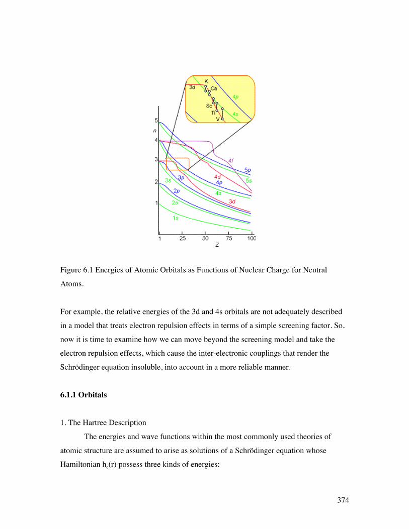
374

Figure 6.1 Energies of Atomic Orbitals as Functions of Nuclear Charge for Neutral

Atoms.

For example, the relative energies of the 3d and 4s orbitals are not adequately described

in a model that treats electron repulsion effects in terms of a simple screening factor. So,

now it is time to examine how we can move beyond the screening model and take the

electron repulsion effects, which cause the inter-electronic couplings that render the

Schrödinger equation insoluble, into account in a more reliable manner.

6.1.1 Orbitals

1. The Hartree Description

The energies and wave functions within the most commonly used theories of

atomic structure are assumed to arise as solutions of a Schrödinger equation whose

Hamiltonian he(r) possess three kinds of energies:

375

1. Kinetic energy, whose average value is computed by taking the expectation value of

the kinetic energy operator – h2/2m ∇2 with respect to any particular solution φJ(r) to the

Schrödinger equation: KE = <φJ| – h2/2m ∇2 |φJ>;

2. Coulombic attraction energy with the nucleus of charge Z: <φJ| -Ze2/r |φJ>;

3. And Coulomb repulsion energies with all of the N-1 other electrons, which are

assumed to occupy other atomic orbitals (AOs) denoted φK, with this energy computed as

ΣK <φJ(r) φK(r’) |(e2/|r-r’|) | φJ(r) φK(r’)>.

The so-called Dirac notation <φJ(r) φK(r’) |(e2/|r-r’|) | φJ(r) φK(r’)> is used to

represent the six-dimensional Coulomb integral JJ,K = ∫|φJ(r)|2 |φK(r’)|2 (e2/|r-r’) dr dr’ that

describes the Coulomb repulsion between the charge density |φJ(r)|2 for the electron in φJ

and the charge density |φK(r’)|2 for the electron in φK. Of course, the sum over K must be

limited to exclude K=J to avoid counting a “self-interaction” of the electron in orbital φJ

with itself.

The total energy εJ of the orbital φJ, is the sum of the above three contributions:

εJ = <φJ| – h2/2m ∇2 |φJ> + <φJ| -Ze2/|r |φJ>

+ ΣK <φJ(r) φK(r’) |(e2/|r-r’|) | φJ(r) φK(r’)>.

This treatment of the electrons and their orbitals is referred to as the Hartree-level of

theory. As stated above, when screened hydrogenic AOs are used to approximate the φJ

and φK orbitals, the resultant εJ values do not produce accurate predictions. For example,

the negative of εJ should approximate the ionization energy for removal of an electron

from the AO φJ. Such ionization potentials (IP s) can be measured, and the measured

values do not agree well with the theoretical values when a crude screening

approximation is made for the AO s.

2. The LACO-Expansion

To improve upon the use of screened hydrogenic AOs, it is most common to

376

approximate each of the Hartree AOs {φK} as a linear combination of so-called basis AOs

{χµ}:

φJ = Σµ CJ,µ χµ.

using what is termed the linear-combination-of-atomic-orbitals (LCAO) expansion. In

this equation, the expansion coefficients {CJ,µ} are the variables that are to be determined

by solving the Schrödinger equation

he φJ = εJ φJ.

After substituting the LCAO expansion for φJ into this Schrödinger equation, multiplying

on the left by one of the basis AOs χν , and then integrating over the coordinates of the

electron in φJ, one obtains

Σµ <χν| he| χµ> CJ,µ = εJ Σµ <χν| χµ> CJ,µ .

This is a matrix eigenvalue equation in which the εJ and {CJ,µ} appear as eigenvalues and

eigenvectors. The matrices <χν| he| χµ> and <χν| χµ> are called the Hamiltonian and

overlap matrices, respectively. An explicit expression for the former is obtained by

introducing the earlier definition of he:

<χν| he| χµ> = <χν| – h2/2m ∇2 |χµ> + <χν| -Ze2/|r |χµ>

+ Ση,γ ΣK CK,η CK,γ <χν(r) χη(r’) |(e2/|r-r’|) | χµ(r) χγ(r’)>.

An important thing to notice about the form of the matrix Hartree equations is that to

compute the Hamiltonian matrix, one must know the LCAO coefficients {CK,γ} of the

orbitals which the electrons occupy. On the other hand, these LCAO coefficients are

supposed to be found by solving the Hartree matrix eigenvalue equations. This paradox

leads to the need to solve these equations iteratively in a so-called self-consistent field

377

(SCF) technique. In the SCF process, one inputs an initial approximation to the {CK,γ}

coefficients. This then allows one to form the Hamiltonian matrix defined above. The

Hartree matrix equations Σµ <χν| he| χµ> CJ,µ = εJ Σµ <χν| χµ> CJ,µ are then solved for new

{CK,γ} coefficients and for the orbital energies {εK}. The new LCAO coefficients of those

orbitals that are occupied are then used to form a new Hamiltonian matrix, after which

the Hartree equations are again solved for another generation of LCAO coefficients and

orbital energies. This process is continued until the orbital energies and LCAO

coefficients obtained in successive iterations do not differ appreciably. Upon such

convergence, one says that a self-consistent field has been realized because the {CK,γ}

coefficients are used to form a Coulomb field potential that details the electron-electron

interactions.

3. AO Basis Sets

a. STOs and GTOs

As noted above, it is possible to use the screened hydrogenic orbitals as the {χµ}.

However, much effort has been expended at developing alternative sets of functions to

use as basis orbitals. The result of this effort has been to produce two kinds of functions

that currently are widely used.

The basis orbitals commonly used in the LCAO process fall into two primary

classes:

1. Slater-type orbitals (STOs) χn,l,m (r,θ,φ) = Nn,l,m,ζ Yl,m (θ,φ) rn-1 e-ζr are

characterized by quantum numbers n, l, and m and exponents (which characterize the

orbital’s radial size ) ζ. The symbol Nn,l,m,ζ denotes the normalization constant.

2. Cartesian Gaussian-type orbitals (GTOs) χa,b,c (r,θ,φ) = N'a,b,c,α xa yb zc exp(-αr2),

are characterized by quantum numbers a, b, and c, which detail the angular shape and

direction of the orbital, and exponents α which govern the radial size.

For both types of AOs, the coordinates r, θ, and φ refer to the position of the

electron relative to a set of axes attached to the nucleus on which the basis orbital is

located. Note that Slater-type orbitals (STO's) are similar to hydrogenic orbitals in the

region close to the nucleus. Specifically, they have a non-zero slope near the nucleus (i.e.,

378

d/dr(exp(-ζr))r=0 = -ζ). In contrast, GTOs, have zero slope near r=0 because

d/dr(exp(-αr2))r=0 = 0. We say that STOs display a cusp at r=0 that is characteristic of the

hydrogenic solutions, whereas GTOs do not.

Although STOs have the proper cusp behavior near nuclei, they are used

primarily for atomic and linear-molecule calculations because the multi-center integrals

<χµ(1) χκ(2)|e2/|r1-r2|| χν(1) χγ(2)> which arise in polyatomic-molecule calculations (we

will discuss these integrals later in this Chapter) cannot efficiently be evaluated when

STOs are employed. In contrast, such integrals can routinely be computed when GTOs

are used. This fundamental advantage of GTOs has lead to the dominance of these

functions in molecular quantum chemistry.

To overcome the primary weakness of GTO functions (i.e., their radial derivatives

vanish at the nucleus), it is common to combine two, three, or more GTOs, with

combination coefficients which are fixed and not treated as LCAO parameters, into new

functions called contracted GTOs or CGTOs. Typically, a series of radially tight,

medium, and loose GTOs are multiplied by contraction coefficients and summed to

produce a CGTO that approximates the proper cusp at the nuclear center (although no

such combination of GTOs can exactly produce such a cusp because each GTO has zero

slope at r = 0).

Although most calculations on molecules are now performed using Gaussian

orbitals, it should be noted that other basis sets can be used as long as they span enough

of the regions of space (radial and angular) where significant electron density resides. In

fact, it is possible to use plane wave orbitals of the form χ (r,θ,φ) = N exp[i(kx r sinθ cosφ

+ ky r sinθ sinφ + kz r cosθ)], where N is a normalization constant and kx , ky , and kz are

quantum numbers detailing the momenta or wavelength of the orbital along the x, y, and

z Cartesian directions. The advantage to using such simple orbitals is that the integrals

one must perform are much easier to handle with such functions. The disadvantage is that

one must use many such functions to accurately describe sharply peaked charge

distributions of, for example, inner-shell core orbitals while still retaining enough

flexibility to also describe the much smoother electron density in the valence regions.

Much effort has been devoted to developing and tabulating in widely available

locations sets of STO or GTO basis orbitals for main-group elements and transition

379

metals. This ongoing effort is aimed at providing standard basis set libraries which:

1. Yield predictable chemical accuracy in the resultant energies.

2. Are cost effective to use in practical calculations.

3. Are relatively transferable so that a given atom's basis is flexible enough to be used for

that atom in various bonding environments (e.g., hybridization and degree of ionization).

b. The Fundamental Core and Valence Basis

In constructing an atomic orbital basis, one can choose from among several

classes of functions. First, the size and nature of the primary core and valence basis must

be specified. Within this category, the following choices are common:

1. A minimal basis in which the number of CGTO orbitals is equal to the number of core

and valence atomic orbitals in the atom.

2. A double-zeta (DZ) basis in which twice as many CGTOs are used as there are core

and valence atomic orbitals. The use of more basis functions is motivated by a desire to

provide additional variational flexibility so the LCAO process can generate molecular

orbitals of variable diffuseness as the local electronegativity of the atom varies. A valence

double-zeta (VDZ) basis has only one CGTO to represent the inner-shell orbitals, but

uses two sets of CGTOs to describe the valence orbitals.

3. A triple-zeta (TZ) basis in which three times as many CGTOs are used as the number

of core and valence atomic orbitals (of course, there are quadruple-zeta and higher-zeta

bases also). Moreover, there are VTZ bases that treat the inner-shell orbitals with one

CGTO and the valence orbitals with three CGTOs.

Optimization of the orbital exponents (ζ’s or α's) and the GTO-to-CGTO

contraction coefficients for the kind of bases described above has undergone considerable

growth in recent years. The theory group at the Pacific Northwest National Labs (PNNL)

offer a world wide web site from which one can find (and even download in a form

prepared for input to any of several commonly used electronic structure codes) a wide

variety of Gaussian atomic basis sets. This site can be accessed at

http://www.emsl.pnl.gov:2080/forms/basisform.html. Professor Kirk Peterson at

Washington State University is involved in the PNNL basis set development project, but

he also hosts his own basis set site at http://tyr0.chem.wsu.edu/~kipeters/basis.html.

380

c. Polarization Functions

One usually enhances any core and valence basis set with a set of so-called

polarization functions. They are functions of one higher angular momentum than appears

in the atom's valence orbital space (e.g., d-functions for C, N, and O and p-functions for

H), and they have exponents (ζ or α) which cause their radial sizes to be similar to the

sizes of the valence orbitals ( i.e., the polarization p orbitals of the H atom are similar in

size to the 1s orbital rather than to the 2s valence orbital of hydrogen). Thus, they are not

orbitals which describe the atom's valence orbital with one higher l-value; such higher-l

valence orbitals would be radially more diffuse.

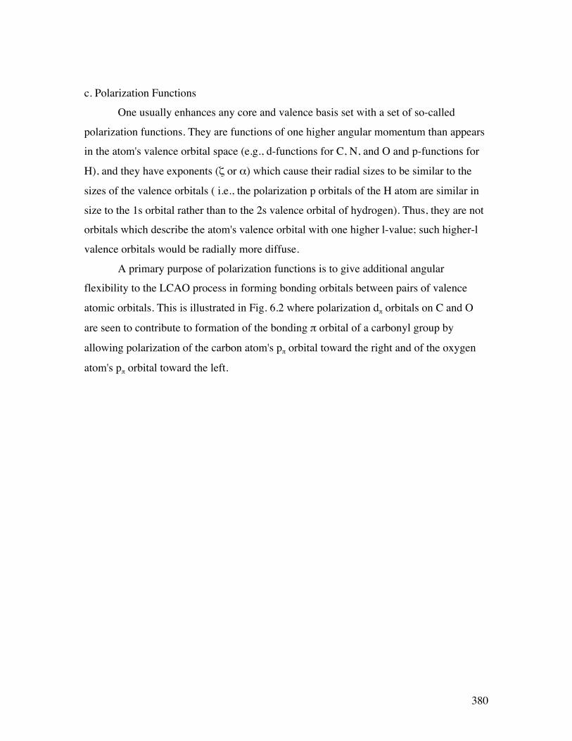
A primary purpose of polarization functions is to give additional angular

flexibility to the LCAO process in forming bonding orbitals between pairs of valence

atomic orbitals. This is illustrated in Fig. 6.2 where polarization dπ orbitals on C and O

are seen to contribute to formation of the bonding π orbital of a carbonyl group by

allowing polarization of the carbon atom's pπ orbital toward the right and of the oxygen

atom's pπ orbital toward the left.

381

Figure 6.2 Oxygen and Carbon Form a π Bond That Uses the Polarization Functions on

Each Atom

Polarization functions are essential in strained ring compounds such as cyclopropane

because they provide the angular flexibility needed to direct the electron density into

regions between bonded atoms, but they are also important in unstrained compounds

when high accuracy is required.

d. Diffuse Functions

When dealing with anions or Rydberg states, one must further augment the AO

C O

C O C O

C O

C O

Carbon p π and d π orbitals combining to form a bent π orbital

Oxygen pπ and d π orbitals combining to form a bent π orbital

π bond formed from C and O bent (polarized) AOs

382

basis set by adding so-called diffuse basis orbitals. The valence and polarization

functions described above do not provide enough radial flexibility to adequately describe

either of these cases. The PNNL web site data base cited above offers a good source for

obtaining diffuse functions appropriate to a variety of atoms as does the site of Prof. Kirk

Peterson.

Once one has specified an atomic orbital basis for each atom in the molecule, the

LCAO-MO procedure can be used to determine the Cµ,i coefficients that describe the

occupied and virtual (i.e., unoccupied) orbitals. It is important to keep in mind that the

basis orbitals are not themselves the SCF orbitals of the isolated atoms; even the proper

atomic orbitals are combinations (with atomic values for the Cµ,i coefficients) of the basis

functions. The LCAO-MO-SCF process itself determines the magnitudes and signs of the

Cν,i. In particular, it is alternations in the signs of these coefficients allow radial nodes to

form.

4. The Hartree-Fock Approximation

Unfortunately, the Hartree approximation discussed above ignores an important

property of electronic wave functions- their permutational antisymmetry. The full

electronic Hamiltonian

H = Σj {- h2/2m ∇2j - Ze2/rj} + 1/2 Σj,k e2/|rj-rk|

is invariant (i.e., is left unchanged) under the operation Pi,j in which a pair of electrons

have their labels (i, j) permuted. We say that H commutes with the permutation operator

Pi,j. This fact implies that any solution ψ to Hψ = Eψ must also be an eigenfunction of Pi,j

Because permutation operators are idempotent, which means that if one applies P twice,

one obtains the identity P P = 1, it can be seen that the eigenvalues of P must be either +1

or –1. That is, if Pψ = cψ, then P P ψ = cc ψ, but PP = 1 means that cc = 1, so c = +1 or –

1.

As a result of H commuting with electron permutation operators and of the

idempotency of P, the eigenfunctions ψ must either be odd or even under the application

of any such permutation. Particles whose wave functions are even under P are called

383

Bose particles or Bosons; those for which ψ is odd are called Fermions. Electrons belong

to the latter class of particles.

The simple spin-orbital product function used in Hartree theory

ψ = Πk=1,N φk

does not have the proper permutational symmetry. For example, the Be atom function

Ψ = 1sα(1) 1sβ(2) 2sα(3) 2sβ(4) is not odd under the interchange of the labels of

electrons 3 and 4; instead one obtains 1sα(1) 1sβ(2) 2sα(4) 2sβ(3). However, such

products of spin-orbitals (i.e., orbitals multiplied by α or β spin functions) can be made

into properly antisymmetric functions by forming the determinant of an NxN matrix

whose row index labels the spin orbital and whose column index labels the electron. For

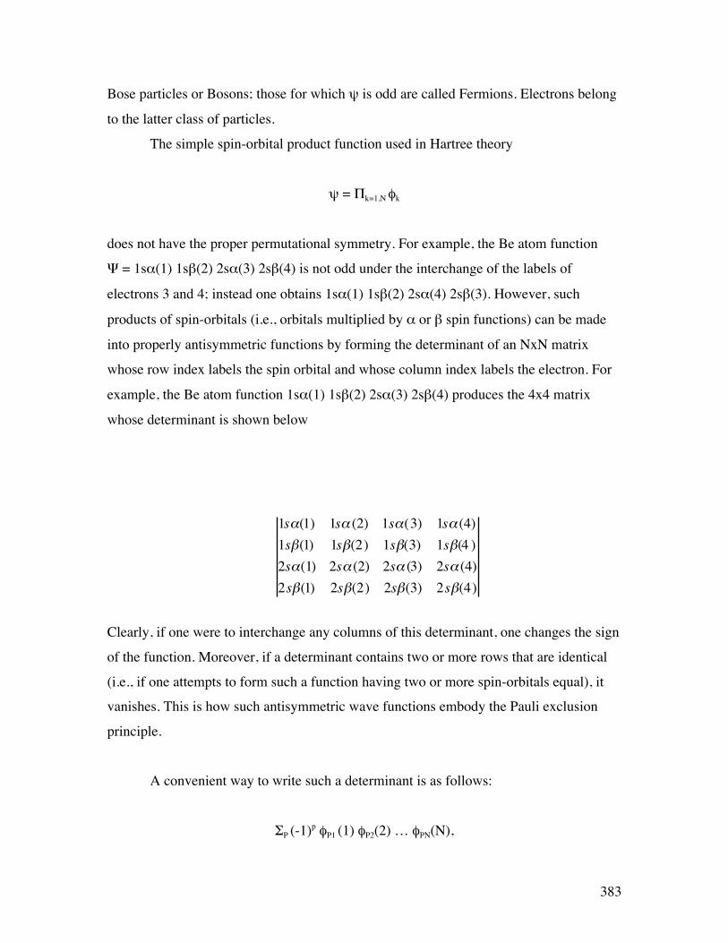
example, the Be atom function 1sα(1) 1sβ(2) 2sα(3) 2sβ(4) produces the 4x4 matrix

whose determinant is shown below

Clearly, if one were to interchange any columns of this determinant, one changes the sign

of the function. Moreover, if a determinant contains two or more rows that are identical

(i.e., if one attempts to form such a function having two or more spin-orbitals equal), it

vanishes. This is how such antisymmetric wave functions embody the Pauli exclusion

principle.

A convenient way to write such a determinant is as follows:

ΣP (-1)p φP1 (1) φP2(2) … φPN(N),

1sα(1) 1sα (2) 1sα(3) 1sα (4)1sβ(1) 1sβ(2) 1sβ(3) 1sβ(4 )2sα(1) 2sα (2) 2sα (3) 2sα (4)2sβ(1) 2sβ(2) 2sβ(3) 2sβ(4)

384

where the sum is over all N! permutations of the N spin-orbitals and the notation (-1)p

means that a –1 is affixed to any permutation that involves an odd number of pair wise

interchanges of spin-orbitals and a +1 sign is given to any that involves an even number.

To properly normalize such a determinental wave function, one must multiply it by

(N!)-1/2. So, the final result is that a wave function of the form

ψ = (N!)-1/2 ΣP (-1)p φP1 (1) φP2(2) … φPN(N),

which is often written in short-hand notation as,

ψ = |φ1 (1) φ2(2) … φN(N)|

has the proper permutational antisymmetry. Note that such functions consist of as sum of

N! factors, all of which have exactly the same number of electrons occupying the same

spin-orbitals; the only difference among the N! terms involves which electron occupies

which spin-orbital. For example, in the 1sα2sα function appropriate to the excited state

of He, one has

ψ = (2)-1/2 {1sα(1) 2sα(2) – 2sα(1) 1sα(2)}

This function is clearly odd under the interchange of the labels of the two electrons, yet

each of its two components has one electron is a 1sα spin-orbital and another electron in

a 2sα spin-orbital.

Although having to make ψ antisymmetric appears to complicate matters

significantly, it turns out that the Schrödinger equation appropriate to the spin-orbitals in

such an antisymmetrized product wave function is nearly the same as the Hartree

Schrödnger equation treated earlier. In fact, if one variationally minimizes the

expectation value of the N-electron Hamiltonian for the above antisymmetric product

wave function subject to the condition that the spin-orbitals are orthonormal

385

<φJ(r)| φk(r)> = δJ,K

one obtains the following equation for the optimal {φJ(r)}:

he φJ = {– h2/2m ∇2 -Ze2/r + ΣK <φK(r’) |(e2/|r-r’|) | φK(r’)>} φJ(r)

- ΣK <φK(r’) |(e2/|r-r’|) | φJ(r’)> φK(r)} = εJ φJ(r).

In this expression, which is known as the Hartree-Fock equation, the same kinetic and

nuclear attraction potentials occur as in the Hartree equation. Moreover, the same

Coulomb potential

ΣK ∫ φK(r’) e2/|r-r’| φK(r’) dr’ = ΣK <φK(r’)|e2/|r-r’| |φK(r’)> = ΣK JK (r)

appears. However, one also finds a so-called exchange contribution to the Hartree-Fock

potential that is equal to ΣL <φL(r’) |(e2/|r-r’|) | φJ(r’)> φL(r) and is often written in short-

hand notation as ΣL KL φJ(r). Notice that the Coulomb and exchange terms cancel for the

L=J case; this causes the artificial self-interaction term JL φL(r) that can appear in the

Hartree equations (unless one explicitly eliminates it) to automatically cancel with the

exchange term KL φL(r) in the Hartree-Fock equations.

To derive the above Hartree-Fock equations, one must make use of the so-called

Slater-Condon rules given in Section 6.1.2 of this Chapter (if you wish to follow all the

details, it is probably wise to pause here and go to Section 6. 1. 2 to learn these rules and

then return here to proceed) to express the Hamiltonian expectation value as

€

<|φ1(1)φ2(2)...φN−1(N −1)φN (N) |H |φ1(1)φ2(2)...φN−1(N −1)φN (N) |>

386

€

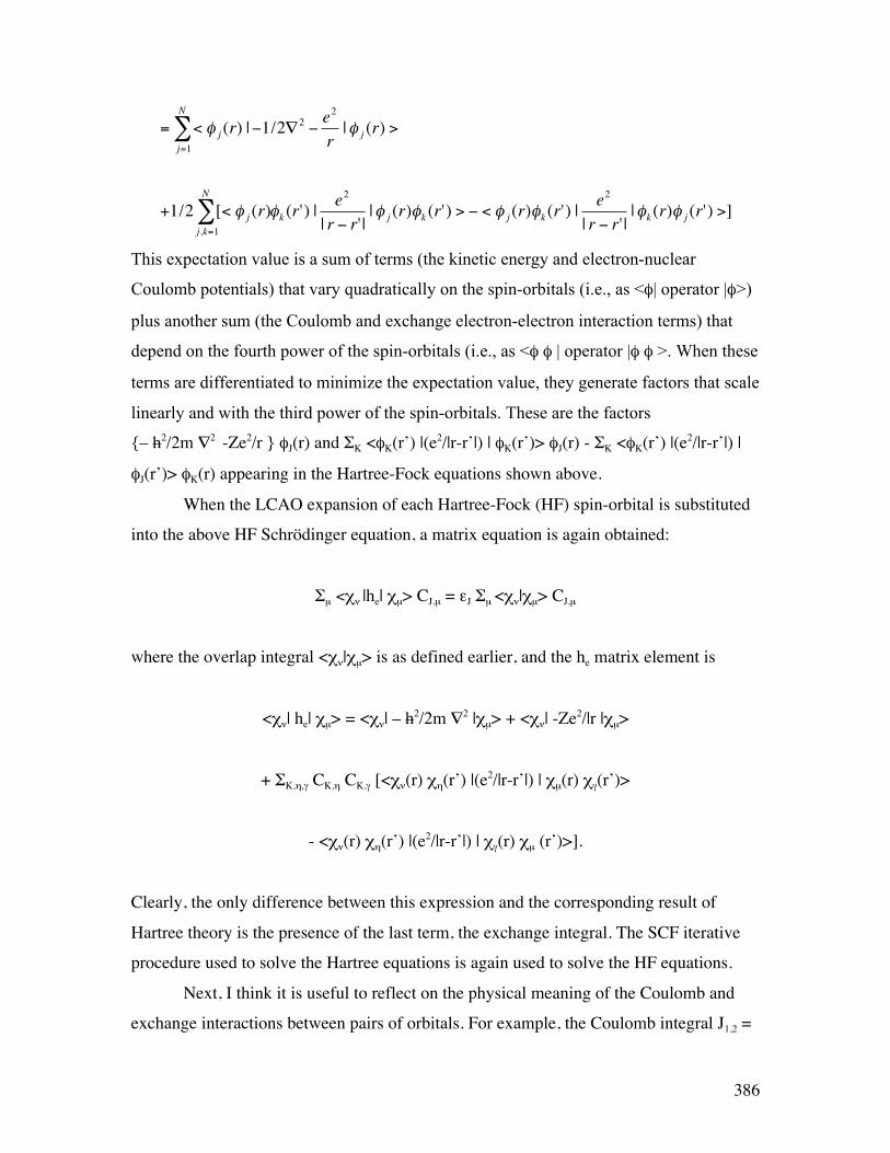
= < φ j (r) |−1/2∇2

j=1

N

∑ −e2

r|φ j (r) >

+1/2 [< φ j (r)j,k=1

N

∑ φk (r') |e2

| r − r' ||φ j (r)φk (r') > − < φ j (r)φk (r') |

e2

| r − r' ||φk (r)φ j (r') >]

This expectation value is a sum of terms (the kinetic energy and electron-nuclear

Coulomb potentials) that vary quadratically on the spin-orbitals (i.e., as <φ| operator |φ>)

plus another sum (the Coulomb and exchange electron-electron interaction terms) that

depend on the fourth power of the spin-orbitals (i.e., as <φ φ | operator |φ φ >. When these

terms are differentiated to minimize the expectation value, they generate factors that scale

linearly and with the third power of the spin-orbitals. These are the factors

{– h2/2m ∇2 -Ze2/r } φJ(r) and ΣK <φK(r’) |(e2/|r-r’|) | φK(r’)> φJ(r) - ΣK <φK(r’) |(e2/|r-r’|) |

φJ(r’)> φK(r) appearing in the Hartree-Fock equations shown above.

When the LCAO expansion of each Hartree-Fock (HF) spin-orbital is substituted

into the above HF Schrödinger equation, a matrix equation is again obtained:

Σµ <χν |he| χµ> CJ,µ = εJ Σµ <χν|χµ> CJ,µ

where the overlap integral <χν|χµ> is as defined earlier, and the he matrix element is

<χν| he| χµ> = <χν| – h2/2m ∇2 |χµ> + <χν| -Ze2/|r |χµ>

+ ΣK,η,γ CK,η CK,γ [<χν(r) χη(r’) |(e2/|r-r’|) | χµ(r) χγ(r’)>

- <χν(r) χη(r’) |(e2/|r-r’|) | χγ(r) χµ (r’)>].

Clearly, the only difference between this expression and the corresponding result of

Hartree theory is the presence of the last term, the exchange integral. The SCF iterative

procedure used to solve the Hartree equations is again used to solve the HF equations.

Next, I think it is useful to reflect on the physical meaning of the Coulomb and

exchange interactions between pairs of orbitals. For example, the Coulomb integral J1,2 =

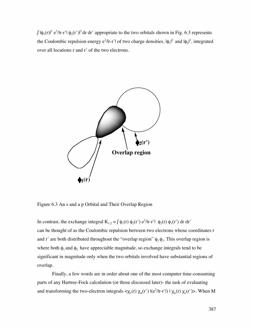
387

∫ |φ1(r)|2 e2/|r-r’| φ2(r’)|2 dr dr’ appropriate to the two orbitals shown in Fig. 6.3 represents

the Coulombic repulsion energy e2/|r-r’| of two charge densities, |φ1|2 and |φ2|2, integrated

over all locations r and r’ of the two electrons.

Figure 6.3 An s and a p Orbital and Their Overlap Region

In contrast, the exchange integral K1,2 = ∫ φ1(r) φ2(r’) e2/|r-r’| φ2(r) φ1(r’) dr dr’

can be thought of as the Coulombic repulsion between two electrons whose coordinates r

and r’ are both distributed throughout the “overlap region” φ1 φ2. This overlap region is

where both φ1 and φ2 have appreciable magnitude, so exchange integrals tend to be

significant in magnitude only when the two orbitals involved have substantial regions of

overlap.

Finally, a few words are in order about one of the most computer time-consuming

parts of any Hartree-Fock calculation (or those discussed later)- the task of evaluating

and transforming the two-electron integrals <χν(r) χη(r’) |(e2/|r-r’|) | χµ(r) χγ(r’)>. When M

φ1(r)

φ2(r')

Overlap region

388

GTOs are used as basis functions, the evaluation of M4/8 of these integrals often poses a

major hurdle. For example, with 500 basis orbitals, there will be of the order of 7.8 x109

such integrals. With each integral requiring 2 words of disk storage (most integrals need

to be evaluated in double precision), this would require at least 1.5 x104 Mwords of disk

storage. Even in the era of modern computers that possess 500 Gby disks, this is a

significant requirement. One of the more important technical advances that is under much

current development is the efficient calculation of such integrals when the product

functions χν(r) χµ(r) and χγ(r’) χη(r’) that display the dependence on the two electrons’

coordinates r and r’ are spatially distant. In particular, so-called multipole expansions of

these product functions are used to obtain more efficient approximations to their integrals

when these functions are far apart. Moreover, such expansions offer a reliable way to

ignore (i.e., approximate as zero) many integrals whose product functions are sufficiently

distant. Such approaches show considerable promise for reducing the M4/8 two-electron

integral list to one whose size scales much less strongly with the size of the AO basis and

form an important component if efforts to achieve CPU and storage needs that scale

linearly with the size of the molecule.

a. Koopmans’ Theorem

The HF-SCF equations he φi = εi φi imply that the orbital energies εi can be

written as:

εi = < φi | he | φi > = < φi | T + V | φi > + Σj(occupied) < φi | Jj - Kj | φi >

= < φi | T + V | φi > + Σj(occupied) [ Ji,j - Ki,j ],

where T + V represents the kinetic (T) and nuclear attraction (V) energies, respectively.

Τhus, εi is the average value of the kinetic energy plus Coulombic attraction to the nuclei

for an electron in φi plus the sum over all of the spin-orbitals occupied in ψ of Coulomb

minus exchange interactions of these electrons with the electron in φi.

389

If φi is an occupied spin-orbital, the j = i term [ Ji,i - Ki,i] disappears in the above

sum and the remaining terms in the sum represent the Coulomb minus exchange

interaction of φi with all of the N-1 other occupied spin-orbitals. If φi is a virtual spin-

orbital, this cancellation does not occur because the sum over j does not include j = i. So,

one obtains the Coulomb minus exchange interaction of φi with all N of the occupied

spin-orbitals in ψ. Hence the energies of occupied orbitals pertain to interactions

appropriate to a total of N electrons, while the energies of virtual orbitals pertain to a

system with N+1 electrons. This difference is very important to understand and to keep in

mind.

Let us consider the following model of the detachment or attachment of an

electron in an N-electron system.

1. In this model, both the parent molecule and the species generated by adding or

removing an electron are treated at the single-determinant level.

2. The Hartree-Fock orbitals of the parent molecule are used to describe both species. It is

said that such a model neglects orbital relaxation (i.e., the re-optimization of the spin-

orbitals to allow them to become appropriate to the daughter species).

Within this model, the energy difference between the daughter and the parent can

be written as follows (φk represents the particular spin-orbital that is added or removed):

for electron detachment:

EN-1 - EN = - εk ;

and for electron attachment:

EN - EN+1 = - εk .

Let’s derive this result for the case in which an electron is added to the N+1st spin-orbital.

Again, using the Slater-Condon rules from Section 6.1.2 of this Chapter, the energy of the

N-electron determinant with spin-orbitals φ1 through φN occupied is

390

EN = Σi(=1,N) < φi | T + V | φi > + Σi>j(=1,N) [ Ji,j - Ki,j ],

which can also be written as

EN = Σi(=1,N) < φi | T + V | φi > + ½ Σi,j(=1,N) [ Ji,j - Ki,j ].

Likewise, the energy of the N+1- electron determinant wave function is

EN+1 = Σi(=1,N+1) < φi | T + V | φi > + ½ Σi,j(=1,N+1) [ Ji,j - Ki,j ].

The difference between these two energies is given by

EN – EN+1 = - < φN+1 | T + V | φN+1 > - ½ Σi(=1,N+1) [ Ji,N+1 - Ki,N+1 ]

- ½ Σj(=1,N+1) [ JN+1,j - KN+1,j ] = - < φN+1 | T + V | φN+1 > - Σi(=1,N+1) [ Ji,N+1 - Ki,N+1 ]

= - εN+1.

That is, the energy difference is equal to minus the expression for the energy of the N+1st

spin-orbital, which was given earlier.

So, within the limitations of the HF, frozen-orbital model, the ionization

potentials (IPs) and electron affinities (EAs) are given as the negative of the occupied and

virtual spin-orbital energies, respectively. This statement is referred to as Koopmans’

theorem; it is used extensively in quantum chemical calculations as a means of estimating

IPs and EAs and often yields results that are qualitatively correct (i.e., ± 0.5 eV).

b. Orbital Energies and the Total Energy

The total HF-SCF electronic energy can be written as:

E = Σi(occupied) < φi | T + V | φi > + Σi>j(occupied) [ Ji,j - Ki,j ]

391

and the sum of the orbital energies of the occupied spin-orbitals is given by:

Σi(occupied) εi = Σi(occupied) < φi | T + V | φi > + Σi,j(occupied) [Ji,j - Ki,j ].

These two expressions differ in a very important way; the sum of occupied orbital

energies double counts the Coulomb minus exchange interaction energies. Thus, within

the Hartree-Fock approximation, the sum of the occupied orbital energies is not equal to

the total energy. This finding teaches us that we can not think of the total electronic

energy of a given orbital occupation in terms of the orbital energies alone. We need to

also keep track of the inter-electron Coulomb and exchange energies.

5. Molecular Orbitals

Before moving on to discuss methods that go beyond the HF model, it is

appropriate to examine some of the computational effort that goes into carrying out a HF

SCF calculation on a molecule. The primary differences that appear when molecules

rather than atoms are considered are

i. The electronic Hamiltonian he contains not only one nuclear-attraction Coulomb

potential Σj Ze2/rj but a sum of such terms, one for each nucleus in the molecule:

Σa Σj Zae2/|rj-Ra|, whose locations are denoted Ra.

ii. One has AO basis functions of the type discussed above located on each nucleus

of the molecule. These functions are still denoted χµ(r-Ra), but their radial and angular

dependences involve the distance and orientation of the electron relative to the particular

nucleus on which the AO is located.

Other than these two changes, performing a SCF calculation on a molecule (or molecular

ion) proceeds just as in the atomic case detailed earlier. Let us briefly review how this

iterative process occurs.

Once atomic basis sets have been chosen for each atom, the one- and two-electron

integrals appearing in the hε and overlap matrices must be evaluated. There are numerous

highly efficient computer codes that allow such integrals to be computed for s, p, d, f, and

even g, h, and i basis functions. After executing one of these so-called integral packages

392

for a basis with a total of M functions, one has available (usually on the computer's hard

disk) of the order of M2/2 one-electron (< χµ | he | χν > and < χµ | χν >) and M4/8 two-

electron (< χµ χδ | χν χκ >) integrals. When treating extremely large atomic orbital

basis sets (e.g., 500 or more basis functions), modern computer programs calculate the

requisite integrals but never store them on the disk. Instead, their contributions to the

<χµ |he|χν> matrix elements are accumulated on the fly after which the integrals are

discarded. This is usually referred to as the direct integral-driven approach.

a. Shapes, Sizes, and Energies of Orbitals

Each molecular spin-orbital (MO) that results from solving the HF SCF equations

for a molecule or molecular ion consists of a sum of components involving all of the

basis AOs:

φj = Σµ Cj,µ χµ.

In this expression, the Cj,µ are referred to as LCAO-MO coefficients because they tell us

how to linearly combine AOs to form the MOs. Because the AOs have various angular

shapes (e.g., s, p, or d shapes) and radial extents (i.e., different orbital exponents), the

MOs constructed from them can be of different shapes and radial sizes. Let’s look at a

few examples to see what I mean.

The first example is rather simple and pertains to two H atoms combining to form

the H2 molecule. The valence AOs on each H atom are the 1s AOs; they combine to form

the two valence MOs (σ and σ*) depicted in Fig. 6.4.

393

Figure 6. 4 Two 1s Hydrogen Atomic Orbitals Combine to Form a Bonding and

Antibonding Molecular Orbital

The bonding MO labeled σ has LCAO-MO coefficients of equal sign for the two 1s AOs,

as a result of which this MO has the same sign near the left H nucleus (A) as near the

right H nucleus (B). In contrast, the antibonding MO labeled σ* has LCAO-MO

coefficients of different sign for the A and B 1s AOs. As was the case in the Hückel or

tight-binding model outlined in Chapter 2, the energy splitting between the two MOs

depends on the overlap <χ1sA|χ1sB> between the two AOs which, in turn, depends on the

distance R between the two nuclei.

An analogous pair of bonding and antibonding MOs arises when two p orbitals

overlap sideways as in ethylene to form π and π* MOs which are illustrated in Fig. 6.5.

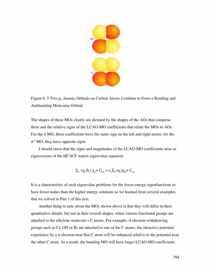
394

Figure 6. 5 Two pπ Atomic Orbitals on Carbon Atoms Combine to Form a Bonding and

Antibonding Molecular Orbital.

The shapes of these MOs clearly are dictated by the shapes of the AOs that comprise

them and the relative signs of the LCAO-MO coefficients that relate the MOs to AOs.

For the π MO, these coefficients have the same sign on the left and right atoms; for the

π* MO, they have opposite signs.

I should stress that the signs and magnitudes of the LCAO-MO coefficients arise as

eigenvectors of the HF SCF matrix eigenvalue equation:

Σµ <χν|he| χµ> Cj,µ = εj Σµ<χν|χµ> Cj,µ

It is a characteristic of such eigenvalue problems for the lower energy eigenfunctions to

have fewer nodes than the higher energy solutions as we learned from several examples

that we solved in Part 1 of this text.

Another thing to note about the MOs shown above is that they will differ in their

quantitative details, but not in their overall shapes, when various functional groups are

attached to the ethylene molecule’s C atoms. For example, if electron-withdrawing

groups such as Cl, OH or Br are attached to one of the C atoms, the attractive potential

experience by a π electron near that C atom will be enhanced relative to the potential near

the other C atom. As a result, the bonding MO will have larger LCAO-MO coefficients

395

Ck,µ belonging to tighter basis AOs χµ on this C atom. This will make the bonding π MO

more radially compact in this region of space, although its nodal character and gross

shape will not change. Alternatively, an electron donating group such as H3C- or t-butyl

attached to one of the C centers will cause the π MO to be more diffuse (by making its

LCAO-MO coefficients for more diffuse basis AOs larger).

In addition to MOs formed primarily of AOs of one type (i.e., for H2 it is primarily s-

type orbitals that form the σ and σ* MOs; for ethylene’s π bond, it is primarily the C 2p

AOs that contribute), there are bonding and antibonding MOs formed by combining

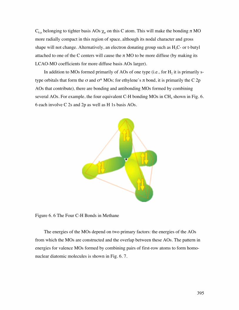
several AOs. For example, the four equivalent C-H bonding MOs in CH4 shown in Fig. 6.

6 each involve C 2s and 2p as well as H 1s basis AOs.

Figure 6. 6 The Four C-H Bonds in Methane

The energies of the MOs depend on two primary factors: the energies of the AOs

from which the MOs are constructed and the overlap between these AOs. The pattern in

energies for valence MOs formed by combining pairs of first-row atoms to form homo-

nuclear diatomic molecules is shown in Fig. 6. 7.

396

Figure 6.7 Energies of the Valence Molecular Orbitals in Homonuclear Diatomics

Involving First-Row Atoms

In this figure, the core MOs formed from the 1s AOs are not shown; only those MOs

formed from 2s and 2p AOs appear. The clear trend toward lower orbital energies as one

moves from left to right is due primarily to the trends in orbital energies of the constituent

AOs. That is, F being more electronegative than N has a lower-energy 2p orbital than

does N.

b. Bonding, Anti-bonding, Non-bonding, and Rydberg Orbitals

As noted above, when valence AOs combine to form MOs, the relative signs of the

combination coefficients determine, along with the AO overlap magnitudes, the MO’s

energy and nodal properties. In addition to the bonding and antibonding MOs discussed

and illustrated earlier, two other kinds of MOs are important to know about.

Non-bonding MOs arise, for example, when an orbital on one atom is not directed

toward and overlapping with an orbital on a neighboring atom. For example, the lone pair

orbitals on H2O or on the oxygen atom of H2C=O are non-bonding orbitals. They still are

described in the LCAO-MO manner, but their Cµ,i coefficients do not contain dominant

contributions from more than one atomic center.

Finally, there is a type of orbital that all molecules possess but that is ignored in

most elementary discussions of electronic structure. All molecules have so-called

397

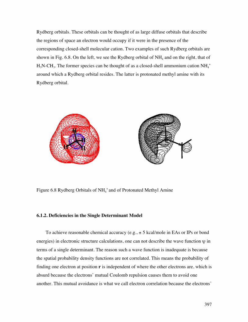
Rydberg orbitals. These orbitals can be thought of as large diffuse orbitals that describe

the regions of space an electron would occupy if it were in the presence of the

corresponding closed-shell molecular cation. Two examples of such Rydberg orbitals are

shown in Fig. 6.8. On the left, we see the Rydberg orbital of NH4 and on the right, that of

H3N-CH3. The former species can be thought of as a closed-shell ammonium cation NH4+

around which a Rydberg orbital resides. The latter is protonated methyl amine with its

Rydberg orbital.

H

H HH

Figure 6.8 Rydberg Orbitals of NH4+ and of Protonated Methyl Amine

6.1.2. Deficiencies in the Single Determinant Model

To achieve reasonable chemical accuracy (e.g., ± 5 kcal/mole in EAs or IPs or bond

energies) in electronic structure calculations, one can not describe the wave function ψ in

terms of a single determinant. The reason such a wave function is inadequate is because

the spatial probability density functions are not correlated. This means the probability of

finding one electron at position r is independent of where the other electrons are, which is

absurd because the electrons’ mutual Coulomb repulsion causes them to avoid one

another. This mutual avoidance is what we call electron correlation because the electrons’

398

motions, as reflected in their spatial probability densities, are correlated (i.e., inter-

related). Let us consider a simple example to illustrate this problem with single

determinant functions. The |1sα(r) 1sβ(r’)| determinant, when written as

|1sα(r) 1sβ(r’)| = 2-1/2{1sα(r) 1sβ(r’) - 1sα(r’) 1sβ(r)}

can be multiplied by itself to produce the 2-electron spin- and spatial- probability density:

P(r, r’) = 1/2{[1sα(r) 1sβ(r’)]2 + [1sα(r’) 1sβ(r)]2 -1sα(r) 1sβ(r’) 1sα(r’) 1sβ(r)

- 1sα(r’) 1sβ(r) 1sα(r) 1sβ(r’)}.

If we now integrate over the spins of the two electrons and make use of

<α|α> = <β|β> = 1, and <α|β> = <β|α> = 0,

we obtain the following spatial (i.e., with spin absent) probability density:

P(r,r’) = |1s(r)|2 |1s(r’)|2.

This probability, being a product of the probability density for finding one electron at r

times the density of finding another electron at r’, clearly has no correlation in it. That is,

the probability of finding one electron at r does not depend on where (r’) the other

electron is. This product form for P(r,r’) is a direct result of the single-determinant form

for ψ, so this form must be wrong if electron correlation is to be accounted for.

1. Electron Correlation

Now, we need to ask how ψ should be written if electron correlation effects are to

be taken into account. As we now demonstrate, it turns out that one can account for

electron avoidance by taking ψ to be a combination of two or more determinants that

differ by the promotion of two electrons from one orbital to another orbital. For example,

in describing the π2 bonding electron pair of an olefin or the ns2 electron pair in alkaline

399

earth atoms, one mixes in doubly excited determinants of the form (π*)2 or np2,

respectively.

Briefly, the physical importance of such doubly-excited determinants can be made

clear by using the following identity involving determinants:

C1 | ..φα φβ..| - C2 | ..φ'α φ'β..|

= C1/2 { | ..( φ - xφ')α ( φ + xφ')β..| - | ..( φ - xφ')β ( φ + xφ')α..| },

where

x = (C2/C1)1/2 .

This identity is important to understand, so please make sure you can work through the

algebra needed to prove it. It allows one to interpret the combination of two determinants

that differ from one another by a double promotion from one orbital (φ) to another (φ') as

equivalent to a singlet coupling (i.e., having αβ-βα spin function) of two different

orbitals (φ - xφ') and (φ + xφ') that comprise what are called polarized orbital pairs. In the

simplest embodiment of such a configuration interaction (CI) description of electron

correlation, each electron pair in the atom or molecule is correlated by mixing in a

configuration state function (CSF) in which that electron pair is doubly excited to a

correlating orbital. A CSF is the minimum combination of determinants needed to

express the proper spin eigenfunction for a given orbital occupation.

In the olefin example mentioned above, the two non-orthogonal polarized orbital

pairs involve mixing the π and π* orbitals to produce two left-right polarized orbitals as

depicted in Fig. 6.9:

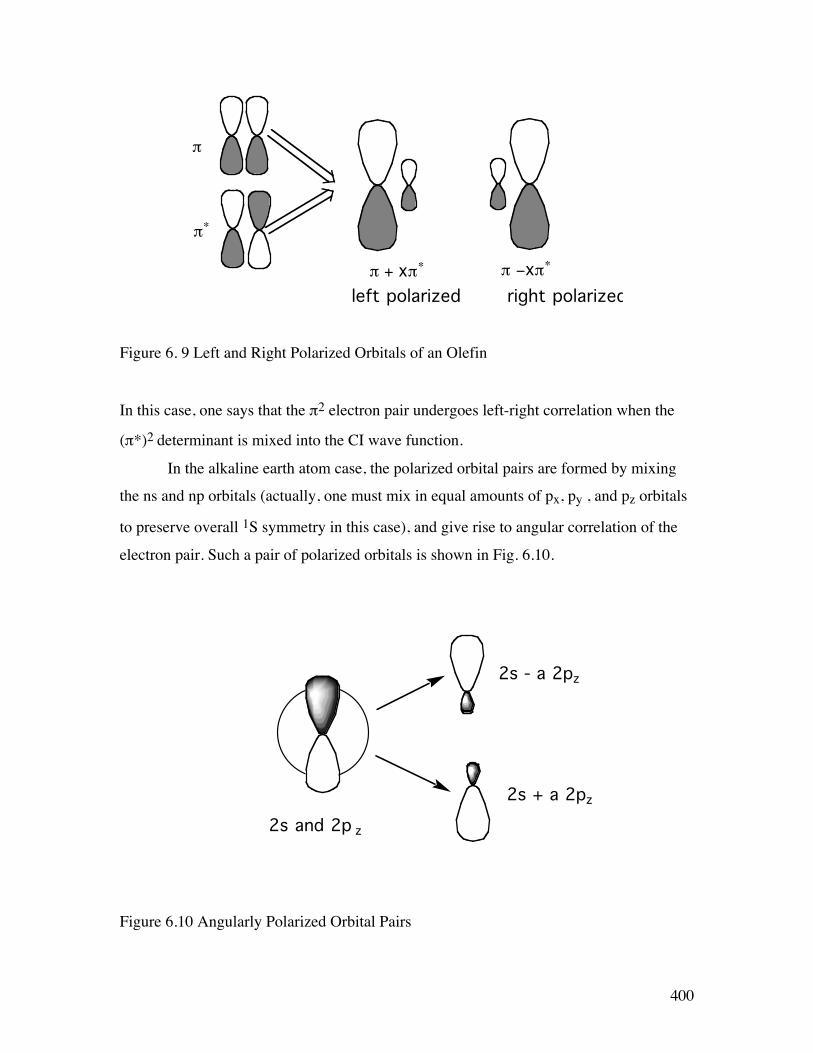
400

currentpoint 192837465

currentpoint

% ChemDraw Laser Prep% CopyRight 1986, 1987, Cambridge Scientific Computing, Inc.userdict/chemdict 145 dict put chemdict begin/version 24 def/b{bind def}bind def/L{load def}b/d/def L/a/add L/al/aload L/at/atan L/cp/closepath L/cv/curveto L/cw/currentlinewidth L/cpt/currentpoint L/dv/div L/dp/dup L/e/exch L/g/get L/gi/getintervalL/gr/grestore L/gs/gsave L/ie/ifelse L/ix/index L/l/lineto L/mt/matrix L/mv/moveto L/m/mul L/n/neg L/np/newpath L/pp/pop L/r/roll L/ro/rotate L/sc/scale L/sg/setgray L/sl/setlinewidth L/sm/setmatrix L/st/stroke L/sp/strokepath L/s/subL/tr/transform L/xl/translate L/S{sf m}b/dA{[3 S]}b/dL{dA dp 0 3 lW m put 0 setdash}d/cR 12 d/wF 1.5 d/aF 10 d/aR 0.25 d/aA 45 d/nH 6 d/o{1 ix}b/rot{3 -1 r}b/x{e d}b/cm mt currentmatrix d/p{tr round e round e itransform}b/Ha{gs np 3 1 rxl dp sc -.6 1.2 p mv 0.6 1.2 p l -.6 2.2 p mv 0.6 2.2 p l cm sm st gr}b/OB{/bS x 3 ix 3 ix xl 3 -1 r s 3 1 r e s o o at ro dp m e dp m a sqrt dp bS dv dp lW 2 m lt{pp lW 2 m}if/bd x}b/DA{np 0 0 mv aL 0 aR aL m 180 aA s 180 aA a arc cp fill}b/OA{np0 cw -2 dv mv aL 0 aR aL m 180 aA s 180 arc 0 cw -2 dv rlineto cp fill}b/SA{aF m lW m/aL x aL 1 aR s m np 0 p mv rad 0 p l gs cm sm st gr}b/CA{aF lW m/aL x aL 1 aR s m 2 dv rad dp m o dp m s dp 0 le{pppp pp}{sqrt at 2 m np rad 0 rad 180 6 -1 r s 180 6 -1 r s arc gs cm sm st gr cpt e at ro}ie}b/AA{np rad 0 rad 180 180 6 -1 r a arc gs cm sm st gr}b/RA{lW m/w x np rad w p mv w w p l rad w n p mv w w n p l w 2 m dp p mv 0 0 pl w 2 m dp n p l st}b/HA{lW m/w x np 0 0 p mv w 2 m dp p l w 2 m w p l rad w p l rad w n p l w 2 m w n p l w 2 m dp n p l cp st}b/Ar1{gs 5 1 r 3 ix 3 ix xl 3 -1 r s 3 1 r e s o o at ro dp m e dp m a sqrt/rad x[{2.25 SA DA}{1.5 SA DA}{1SA DA}{cw 5 m sl 3.375 SA DA}{cw 5 m sl 2.25 SA DA}{cw 5 m sl 1.5 SA DA}{270 CA DA}{180 CA DA}{120 CA DA}{90 CA DA}{3 RA}{3 HA}{1 -1 sc 270 CA DA}{1 -1 sc 180 CA DA}{1 -1 sc 120 CA DA}{1 -1 sc 90 CA DA}{6RA}{6 HA}{dL 2.25 SA DA}{dL 1.5 SA DA}{dL 1 SA DA}{2.25 SA OA}{1.5 SA OA}{1 SA OA}{1 -1 sc 2.25 SA OA}{1 -1 sc 1.5 SA OA}{1 -1 sc 1 SA OA}{270 CA OA}{180 CA OA}{120 CA OA}{90 CA OA}{1 -1 sc 270 CA OA}{1-1 sc 180 CA OA}{1 -1 sc 120 CA OA}{1 -1 sc 90 CA OA}{1 -1 sc 270 AA}{1 -1 sc 180 AA}{1 -1 sc 120 AA}{1 -1 sc 90 AA}]e g exec gr}b/ac{arcto 4{pp}repeat}b/pA 32 d/rO{4 lW m}b/Ac{0 0 px dp m py dp m a sqrt 0 360 arc cm sm gs sg fill grst}b/OrA{py px at ro px dp m py dp m a sqrt dp rev{neg}if sc}b/Ov{OrA 1 0.4 sc 0 0 1 0 360 arc cm sm gs sg fill gr st}b/Asc{OrA 1 27 dv dp sc}b/LB{9 -6 mv 21 -10 27 -8 27 0 cv 27 8 21 10 9 6 cv -3 2 -3 -2 9 -6 cv cp}b/DLB{0 0 mv -4.8 4.8 l-8 8 -9.6 12 -9.6 16.8 cv -9.6 21.6 -8 24.6 -4.8 25.8 cv -1.6 27 1.6 27 4.8 25.8 cv 8 24.6 9.6 21.6 9.6 16.8 cv 9.6 12 8 8 4.8 4.8 cv cp}b/ZLB{LB}b/Ar{dp 39 lt{Ar1}{gs 5 1 r o o xl 3 -1 r e s 3 1 r s e o 0 lt o 0 lt ne/rev xdp 0 lt{1 -1 sc neg}if/py x dp 0 lt{-1 1 sc neg}if/px x np[{py 16 div dup 2 S lt{pp 2 S}if/lp x lp 0 p mv 0 0 p l 0 py p l lp py p l px lp s 0 p mv px 0 p l px py p l px lp s py p l cm sm st}{py 16 div dup 2 S lt{pp 2 S}if/lp x lp 0 p mv 0 0 0 py lp ac0 py 2 dv lp neg o lp ac 0 py 2 dv 0 py lp ac 0 py lp py lp ac px lp s 0 p mv px 0 px py lp ac px py 2 dv px lp a o lp ac px py 2 dv px py lp ac px py px lp s py lp ac cm sm st}{py dp 2 dv py 180 pA s 180 pA a arc st np px py s py 2 dvpy pA dp neg arcn st}{0 0 p mv 0 py p l px py p l px 0 p l cp cm sm st}{px lW 2 dv a lW -2 dv p mv rO dp rlineto px lW 2 dv a rO a py lW 2 dv a rO a p l rO lW -2 dv a py lW 2 dv a rO a p l lW -2 dv py lW 2 dv a p l 0 py p l px py p l px 0 p l cp fill0 0 p mv 0 py p l px py p l px 0 p l cp cm sm st}{0 rO p mv 0 py px py rO ac px py px 0 rO ac px 0 0 0 rO ac 0 0 0 py rO ac cp cm sm st}{rO py p mv rO rO xl 0 py px py rO ac px py px 0 rO ac px 0 0 0 rO ac rO neg dp xl px py 0 py rO accp fill 0 rO p mv 0 py px py rO ac px py px 0 rO ac px 0 0 0 rO ac 0 0 0 py rO ac cp st}{1.0 Ac}{0.5 Ac}{1.0 Ov}{0.5 Ov}{Asc LB gs 1 sg fill gr cm sm st}{Asc LB gs 0.5 sg fill gr cm sm st}{Asc LB gs 0.5 sg fill gr gs cm sm st grnp -1 -1 sc LB gs 1 sg fill gr cm sm st}{Asc LB gs 0.5 sg fill gr gs cm sm st gr np -0.4 -0.4 sc LB gs 1 sg fill gr cm sm st}{Asc LB gs 1 sg fill gr gs cm sm st gr np -0.4 -0.4 dp sc LB gs 0.5 sg fill gr cm sm st}{Asc DLB -1 -1 sc DLB gs 1 sg fill grgs cm sm st gr np 90 ro DLB -1 -1 sc DLB gs 0.5 sg fill gr cm sm st}{Asc gs -1 -1 sc ZLB gs 1 sg fill gr cm sm st gr gs 0.3 1 sc 0 0 12 0 360 arc gs 0.5 sg fill gr cm sm st gr ZLB gs 1 sg fill gr cm sm st}{Asc gs -1 -1 sc ZLB gs 0.5 sgfill gr cm sm st gr gs 0.3 1 sc 0 0 12 0 360 arc gs 1 sg fill gr cm sm st gr ZLB gs 0.5 sg fill gr cm sm st}{0 0 p mv px py p l cm sm st}{gs bW 0 ne{bW}{5 lW m}ie sl 0 0 p mv px py p l cm sm st gr}{gs dL 0 0 p mv px py p l cm sm st gr}{OrA 1 16 dv dp sc0 1 p mv 0 0 1 0 1 ac 8 0 8 -1 1 ac 8 0 16 0 1 ac 16 0 16 1 1 ac cm sm st}]e 39 s g exec gr}ie}b/Cr{0 360 np arc st}b/DS{np p mv p l st}b/DD{gs dL DS gr}b/DB{gs 12 OB bW 0 ne{bW}{2 bd m}ie sl np 0 0 p mv 0 p l st gr}b/ap{e 3 ix ae 2 ix a}b/PT{8 OB 1 sc 0 bd p 0 0 p 3 -1 r s 3 1 r e s e 0 0 p mv 1 0 p l 0 0 p ap mv 1 0 p ap l e n e n 0 0 p ap mv 1 0 p ap l pp pp}b/DT{gs np PT cm sm st gr}b/Bd{[{pp}{[{DS}{DD}{gs 12 OB np bW 0 ne{bW 2 dv/bd x}if dp nH dv dp 3 -1 ro 2 dv s{dp bd p mv bd n p l}for st gr}{gs 12 OB 1 sc np bW 0 ne{bW 2 dv/bd x}if 1 1 nH 1 s{nH dv dp bd m wF m o o p mv n p l}for cm sm st gr}{pp}{DB}{gs 12 OB np 0 lW 2 dv o o n p mv p l bW 0 ne{bW 2 dv}{bd}ie wF m o o p l n p lcp fill gr}{pp}{gs 12 OB/bL x bW 0 ne{bW 2 dv/bd x}if np 0 0 p mv bL bd 4 m dv round 2 o o lt{e}if pp cvi/nSq x bL nSq 2 m dv dp sc nSq{.135 .667 .865 .667 1 0 rcurveto .135 -.667 .865 -.667 1 0 rcurveto}repeat cm sm st gr}]o 1 g 1 s g e 2 4 gi al pp5 -1 r exec}{al pp 8 ix 1 eq{DD}{DS}ie 5 -1 r 2 eq{DB}{DS}ie pp}{2 4 gi al pp DT}]o 0 g g exec}b/CS{p mv p l cw lW cW 2 m a sl sp sl}b/cB{12 OB 0 0 p mv 0 p l cm sm cw bW 0 ne{bW}{bd 2 m}ie cW 2 m a sl sp sl}b/CW{12 OB 1 sc cW lW 2 dva 0 o p mv 0 e n p l bW 0 ne{bW 2 dv}{bd}ie wF m cW a 1 o n p l 1 e p l cp cm sm}b/CB{np[{[{CS}{CS}{cB}{CW}{pp}{cB}{CW}{pp}{cB}]o 1 g 1 s g e 2 4 gi al pp 5 -1 r exec}{al pp p mv p l CS pp pp}{2 4 gi al pp PT cm sm cw cW 2 m sl sp sl}]o0 g 1 s g exec clip}b/Ct{bs rot g bs rot g gs o CB CB 1 setgray clippath fill 0 setgray Bd gr}b/wD 18 dict d/WI{wx dx ne{wy dy s wx dx s dv/m1 x wy m1 wx m s/b1 x}if lx ex ne{ly ey s lx ex s dv/m2 x ly m2 lx m s/b2 x wx dx ne{b2 b1 s m1 m2 s dv}{wx}iedp m2 m b2 a}{ex n dp m1 m b1 a}ie}b/WW{gs wD begin bs e g 2 4 gi al pp o o xl 4 -1 r 3 -1 r s/wx x s/wy x bs e g 2 4 gi al pp 4 -1 r 3 -1 r s/lx x s/ly x 0 bW 2 dv wF m o o wy wx at mt ro tr/dy x/dx x ly lx at mt ro tr n/ey x n/ex x np wxwy p mv WI p l ex n/ex x ey n/ey x dx n/dx x dy n/dy x lx ly p l WI p l cp fill end gr}b/In{px dx ne{py dy s px dx s dv/m1 x py m1 px m s/b1 x}if lx 0 ne{ly lx dv/m2 x ly ey s m2 lx ex s m s/b2 x px dx ne{b2 b1 s m1 m2 s dv}{px}iedp m2 m b2 a}{ex n dp m1 m b1 a}ie}b/BW{wD begin bs e g/wb x bs e g/bb x wb 4 g/cX x wb 5 g/cY x bb 4 g cX eq bb 5 g cY eq and{bb 2 g bb 3 g}{bb 4 g bb 5 g}ie cY s/ly x cX s/lx x/wx wb 2 g cX s d/wy wb 3 g cY s d 0 bW 2 dv ly lx at mt ro tr/ey x/ex x0 bW 2 dv wF m wy wx at mt ro tr/dy x/dx x 0 lW 2 dv wy wx at mt ro tr wy a/py x wx a/px x gs cX cY xl np px py p mv In p l lx ex s ly ey s p l ex n/ex x ey n/ey x dx n/dx x dy n/dy x wx 2 m px s/px x wy 2 m py s/py x lx ex s ly ey s p lIn p l px py p l cp fill gr end}b/Db{bs{dp type[]type eq{dp 0 g 2 eq{gs dp 1 g 1 eq{dL}if 6 4 gi al pp DS gr}{dp 0 g 3 eq{2 4 gi al pp DT}{pp}ie}ie}{pp}ie}forall}b/I{counttomark dp 1 gt{2 1 rot{-1 r}for}{pp}ie}b/DSt{o/iX x dp/iY x o/cXx dp/cY x np p mv counttomark{bs e g 2 4 gi al pp o cX ne o cY ne or{4 1 r 4 1 r}if pp pp o/cX x dp/cY x o iX eq o iY eq and{pp pp cp}{p l}ie}repeat pp st}b/SP{gs/sf x/lW x/bW x/cW x count 9 ge 7 ix 192837465 eq and{ 7 -1 r pp6 -2 r o o xl 7 -1 r s e 7 -1 r s e 5 -1 r dv neg e 5 -1 r dv neg e sc neg e neg e xl}{xl pp pp}ifelse 1 1 S dv dp sc cm currentmatrix pp lW sl 4.0 setmiterlimit np}b end358 175 65 25 40 68 14 20 chemdict begin SP 1960 1800 1960 1160 52 Ar 2380 1800 2380 1160 52 Ar 1980 3340 1980 2700 52 Ar 2420 2080 2420 2720 52 Ar 3660 1920 2600 1120 10 Ar 3640 2080 2560 2740 10 Ar 4380 3060 4380 1980 52 Ar 4900 2400 4900 1980 52 Ar 6900 3040 6900 1960 52 Ar 6380 2380 6380 1960 52 Ar /bs[]d Db gr end

left polarized right polarizedπ −xπ∗π + xπ∗

π∗

π

Figure 6. 9 Left and Right Polarized Orbitals of an Olefin

In this case, one says that the π2 electron pair undergoes left-right correlation when the

(π*)2 determinant is mixed into the CI wave function.

In the alkaline earth atom case, the polarized orbital pairs are formed by mixing

the ns and np orbitals (actually, one must mix in equal amounts of px, py , and pz orbitals

to preserve overall 1S symmetry in this case), and give rise to angular correlation of the

electron pair. Such a pair of polarized orbitals is shown in Fig. 6.10.

2s and 2p z

2s + a 2pz

2s - a 2pz

Figure 6.10 Angularly Polarized Orbital Pairs

401

More specifically, the following four determinants are found to have the largest

amplitudes in ψ for Be:

ψ ≅ C1 |1s22s2 | - C2 [|1s22px2 | +|1s22py2 | +|1s22pz2 |].

The fact that the latter three terms possess the same amplitude C2 is a result of the

requirement that a state of 1S symmetry is desired. It can be shown that this function is

equivalent to:

ψ ≅ 1/6 C1 |1sα1sβ{[(2s-a2px)α(2s+a2px)β - (2s-a2px)β(2s+a2px)α]

+[(2s-a2py)α(2s+a2py)β - (2s-a2py)β(2s+a2py)α]

+[(2s-a2pz)α(2s+a2pz)β - (2s-a2pz)β(2s+a2pz)α] |,

where a = 3C2/C1 .

Here two electrons occupy the 1s orbital (with opposite, α and β spins), and are

thus not being treated in a correlated manner, while the other pair resides in 2s/2p

polarized orbitals in a manner that instantaneously correlates their motions. These

polarized orbital pairs (2s ± a 2px,y, or z) are formed by combining the 2s orbital with

the 2px,y, or z orbital in a ratio determined by C2/C1.

This ratio C2/C1 can be shown using perturbation theory to be proportional to the

magnitude of the coupling <1s22s2 |H|1s22p2 > matrix element between the two

configurations involved and inversely proportional to the energy difference

[<1s22s2H|1s22s2> - <1s22p2|H|1s22p2>] between these configurations. In general,

configurations that have similar Hamiltonian expectation values and that are coupled

strongly give rise to strongly mixed (i.e., with large |C2/C1| ratios) polarized orbital pairs.

II. Later in this Chapter, you will learn how to evaluate Hamiltonian matrix elements

between pairs of antisymmetric wave functions. If you are anxious to learn this now,

402

go to the subsection entitled The Slater-Condon Rules and read that before returning

here.

In each of the three equivalent terms in the alkaline earth wave function, one of

the valence electrons moves in a 2s+a2p orbital polarized in one direction while the other

valence electron moves in the 2s-a2p orbital polarized in the opposite direction. For

example, the first term [(2s-a2px)α(2s+a2px)β - (2s-a2px)β(2s+a2px)α] describes one

electron occupying a 2s-a2px polarized orbital while the other electron occupies the

2s+a2px orbital. The electrons thus reduce their Coulomb repulsion by occupying

different regions of space; in the SCF picture 1s22s2, both electrons reside in the same 2s

region of space. In this particular example, the electrons undergo angular correlation to

avoid one another.

The use of doubly excited determinants is thus seen as a mechanism by which ψ

can place electron pairs, which in the single-configuration picture occupy the same

orbital, into different regions of space (i.e., each one into a different member of the

polarized orbital pair) thereby lowering their mutual Coulomb repulsion. Such electron

correlation effects are extremely important to include if one expects to achieve

chemically meaningful accuracy (i.e., ± 5 kcal/mole).

2. Essential Configuration Interaction

There are occasions in which the inclusion of two or more determinants in ψ is

essential to obtaining even a qualitatively correct description of the molecule’s electronic

structure. In such cases, we say that we are including essential correlation effects. To

illustrate, let us consider the description of the two electrons in a single covalent bond

between two atoms or fragments that we label X and Y. The fragment orbitals from

which the bonding σ and antibonding σ* MOs are formed we will label sX and sY,

respectively.

Several spin- and spatial- symmetry adapted 2-electron determinants (i.e., CSFs)

can be formed by placing two electrons into the σ and σ* orbitals. For example, to

describe the singlet determinant corresponding to the closed-shell σ2 orbital occupancy, a

single Slater determinant

403

1Σ (0) = |σα σβ| = (2)-1/2 { σα(1) σβ(2) - σβ(1) σα(2) }

suffices. An analogous expression for the (σ*)2 determinant is given by

1Σ** (0) = | σ*ασ*β | = (2)−1/2 { σ*α (1) σ*β (2) - σ*α (2) σ*β (1) }.

Also, the MS = 1 component of the triplet state having σσ* orbital occupancy can be

written as a single Slater determinant:

3Σ* (1) = |σα σ*α| = (2)-1/2 { σα(1) σ* α(2) - σ* α(1) σα(2) },

as can the MS = -1 component of the triplet state

3Σ*(-1) = |σβ σ*β| = (2)-1/2 { σβ(1) σ* β(2) - σ* β(1) σβ(2) }.

However, to describe the singlet and MS = 0 triplet states belonging to the σσ*

occupancy, two determinants are needed:

1Σ* (0) =

€

12|σασ *β |− |σβσ *α |[ ]

is the singlet and

3Σ*(0) =

€

12|σασ *β |+ |σβσ *α |[ ]

is the triplet (note, you can obtain this MS = 0 triplet by applying S- = S-(1) + S-(2) to the

MS = 1 triplet). In each case, the spin quantum number S, its z-axis projection MS , and

the Λ quantum number are given in the conventional 2S+1Λ(MS) term symbol notation.

404

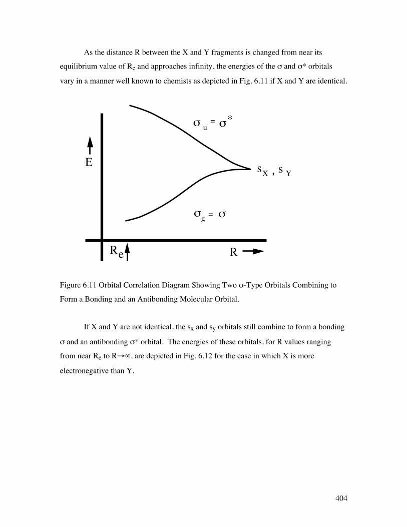
As the distance R between the X and Y fragments is changed from near its

equilibrium value of Re and approaches infinity, the energies of the σ and σ* orbitals

vary in a manner well known to chemists as depicted in Fig. 6.11 if X and Y are identical.

E

RRe

*σuσ =

σσg =

YsXs ,

Figure 6.11 Orbital Correlation Diagram Showing Two σ-Type Orbitals Combining to

Form a Bonding and an Antibonding Molecular Orbital.

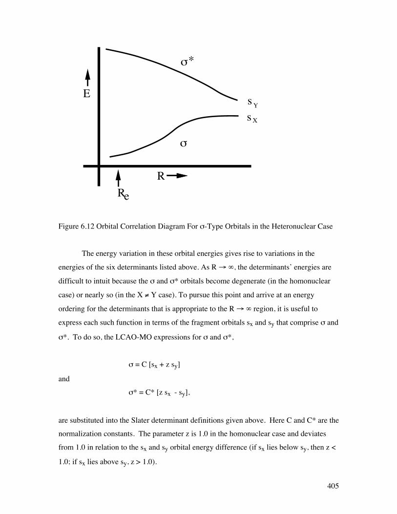
If X and Y are not identical, the sx and sy orbitals still combine to form a bonding

σ and an antibonding σ* orbital. The energies of these orbitals, for R values ranging

from near Re to R→∞, are depicted in Fig. 6.12 for the case in which X is more

electronegative than Y.

405

Re

E

R

*σ

σ

sYsX

Figure 6.12 Orbital Correlation Diagram For σ-Type Orbitals in the Heteronuclear Case

The energy variation in these orbital energies gives rise to variations in the

energies of the six determinants listed above. As R → ∞, the determinants’ energies are

difficult to intuit because the σ and σ* orbitals become degenerate (in the homonuclear

case) or nearly so (in the X ≠ Y case). To pursue this point and arrive at an energy

ordering for the determinants that is appropriate to the R → ∞ region, it is useful to

express each such function in terms of the fragment orbitals sx and sy that comprise σ and

σ*. To do so, the LCAO-MO expressions for σ and σ*,

σ = C [sx + z sy]

and

σ* = C* [z sx - sy],

are substituted into the Slater determinant definitions given above. Here C and C* are the

normalization constants. The parameter z is 1.0 in the homonuclear case and deviates

from 1.0 in relation to the sx and sy orbital energy difference (if sx lies below sy, then z <

1.0; if sx lies above sy, z > 1.0).

406

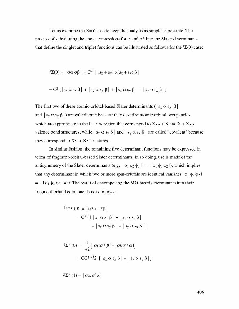
Let us examine the X=Y case to keep the analysis as simple as possible. The

process of substituting the above expressions for σ and σ* into the Slater determinants

that define the singlet and triplet functions can be illustrated as follows for the 1Σ(0) case:

1Σ(0) = σα σβ = C2 (sx + sy) α(sx + sy) β

= C2 [sx α sx β + sy α sy β + sx α sy β + sy α sx β]

The first two of these atomic-orbital-based Slater determinants (sx α sx β

and sy α sy β) are called ionic because they describe atomic orbital occupancies,

which are appropriate to the R → ∞ region that correspond to X

€

•• + X and X + X

€

••

valence bond structures, while sx α sy β and sy α sx β are called "covalent" because

they correspond to X• + X• structures.

In similar fashion, the remaining five determinant functions may be expressed in

terms of fragment-orbital-based Slater determinants. In so doing, use is made of the

antisymmetry of the Slater determinants (e.g., | φ1 φ2 φ3 | = - | φ1 φ3 φ2 |), which implies

that any determinant in which two or more spin-orbitals are identical vanishes | φ1 φ2 φ2 |

= - | φ1 φ2 φ2 | = 0. The result of decomposing the MO-based determinants into their

fragment-orbital components is as follows:

1Σ** (0) = σ*α σ*β

= C*2 [ sx α sx β + sy α sy β

− sx α sy β − sy α sx β]

1Σ* (0) =

€

12|σασ *β |− |σβσ *α |[ ]

= CC* 2 [sx α sx β − sy α sy β]

3Σ* (1) = σα σ*α

407

= CC* 2sy α sx α

3Σ* (0) =

€

12|σασ *β |+ |σβσ *α |[ ]

=CC* 2 [sy α sx β − sx α sy β]

3Σ* (-1) = σα σ*α

= CC* 2sy β sx β

These decompositions of the six valence determinants into fragment-orbital or

valence bond components allow the R = ∞ energies of these states to specified. For

example, the fact that both 1Σ and 1Σ** contain 50% ionic and 50% covalent structures

implies that, as R → ∞, both of their energies will approach the average of the covalent

and ionic atomic energies 1/2 [E (X•) + E (X•) + E (X) + E ( X

€

••) ]. The 1Σ* energy

approaches the purely ionic value E (X)+ E (X

€

••) as R → ∞. The energies of 3Σ*(0), 3Σ*(1) and 3Σ*(-1) all approach the purely covalent value E (X•) + E (X•) as R→∞.

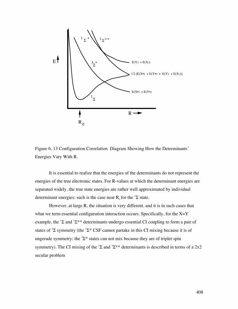
The behaviors of the energies of the six valence determinants as R varies are

depicted in Fig. 6.13 for situations in which the homolytic bond cleavage is energetically

favored (i.e., for which E (X•) + E (X•) < E (X) +E ( X

€

••)).

408

Re

E

1Σ∗∗

R

1Σ

1 Σ ∗

∗Σ3 E(Y) + E(X:)

1/2 [E(X•) + E(Y•) + E(Y) + E(X :)]

E(X•) + E(Y•)

Figure 6. 13 Configuration Correlation Diagram Showing How the Determinants’

Energies Vary With R.

It is essential to realize that the energies of the determinants do not represent the

energies of the true electronic states. For R-values at which the determinant energies are

separated widely, the true state energies are rather well approximated by individual

determinant energies; such is the case near Re for the 1Σ state.

However, at large R, the situation is very different, and it is in such cases that

what we term essential configuration interaction occurs. Specifically, for the X=Y

example, the 1Σ and 1Σ** determinants undergo essential CI coupling to form a pair of

states of 1Σ symmetry (the 1Σ* CSF cannot partake in this CI mixing because it is of

ungerade symmetry; the 3Σ* states can not mix because they are of triplet spin

symmetry). The CI mixing of the 1Σ and 1Σ** determinants is described in terms of a 2x2

secular problem

409

€

<1 Σ |Η |1 Σ > <1 Σ |Η |1 Σ∗∗ >

<1 Σ∗∗ |Η |1 Σ > <1 Σ∗∗ |Η |1 Σ∗∗ >

A

B = E

A

B

The diagonal entries are the determinants’ energies depicted in Fig. 6.13. The off-

diagonal coupling matrix elements can be expressed in terms of an exchange integral

between the σ and σ* orbitals:

〈1ΣH1Σ**〉 = 〈σα σβHσ*α σ*β〉 = 〈σσ1

r12 σ*σ*〉 = Κσσ*

Later in this Chapter, you will learn how to evaluate Hamiltonian matrix elements

between pairs of antisymmetric wave functions and to express them in terms of one- and

two-electron integrals. If you are anxious to learn this now, go to the subsection entitled

the Slater-Condon Rules and read that before returning here.

At R → ∞, where the 1Σ and 1Σ** determinants are degenerate, the two solutions

to the above CI matrix eigenvalue problem are:

E+_ =1/2 [ E (X•) + E (X•) + E (X)+ E (X

€

••) ] -+ 〈σσ 1

r12 σ* σ*〉

with respective amplitudes for the 1Σ and 1Σ** CSFs given by

A+- = ±

12 ; B

+- = -+

12 .

The first solution thus has

ψ− = 12 [σα σβ - σ*α σ*β]

which, when decomposed into atomic orbital components, yields

410

ψ− = 12 [ sxα syβ - sxβ syα].

The other root has

ψ+ = 12 [σα σβ + σ*α σ*β]

= 12 [ sxα sxβ + sy α syβ].

So, we see that 1Σ and 1Σ**, which both contain 50% ionic and 50% covalent parts,

combine to produce ψ_ which is purely covalent and ψ+ which is purely ionic.

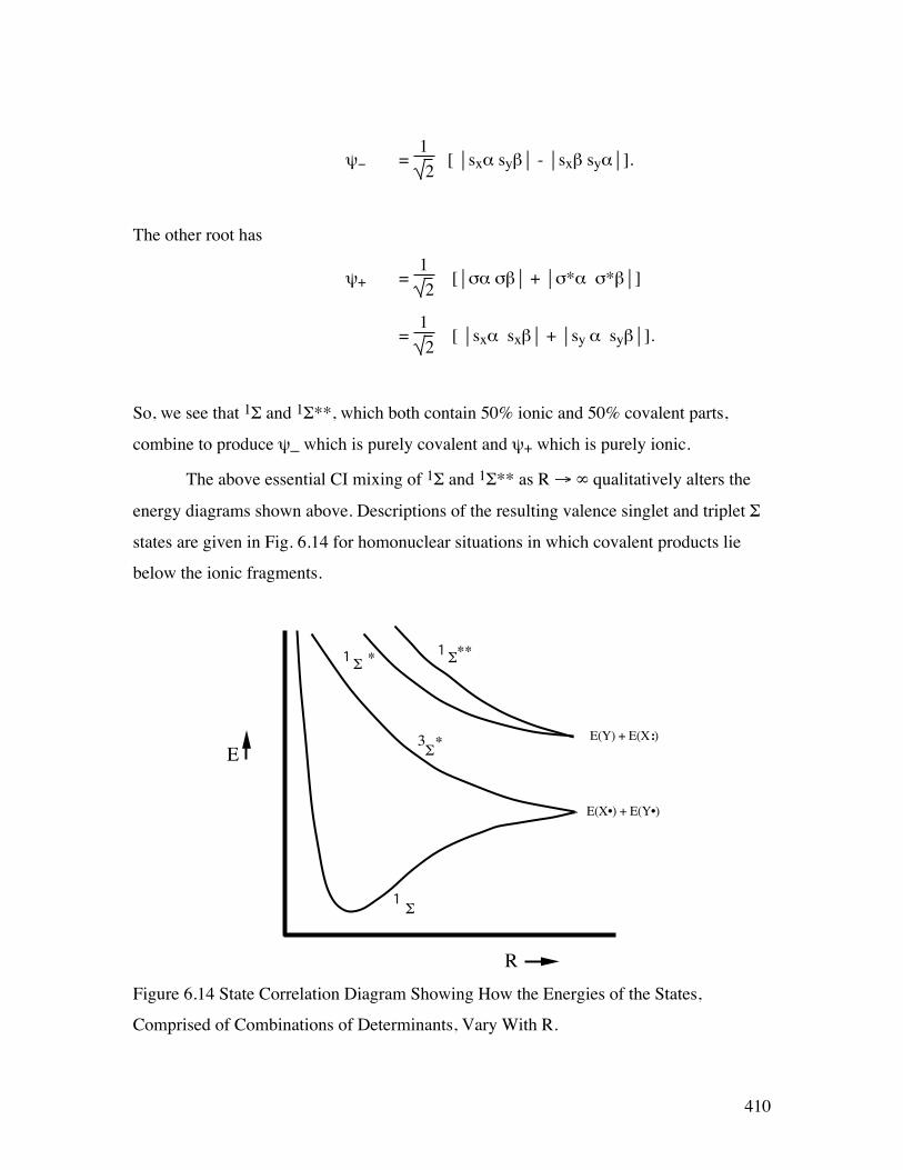
The above essential CI mixing of 1Σ and 1Σ** as R → ∞ qualitatively alters the

energy diagrams shown above. Descriptions of the resulting valence singlet and triplet Σ

states are given in Fig. 6.14 for homonuclear situations in which covalent products lie

below the ionic fragments.

∗∗1Σ

E

R

1Σ ∗

∗Σ3

1Σ

E(Y) + E(X:)

E(X•) + E(Y•)

Figure 6.14 State Correlation Diagram Showing How the Energies of the States,

Comprised of Combinations of Determinants, Vary With R.

411

3. Various Approaches to Electron Correlation

There are numerous procedures currently in use for determining the best Born-

Oppenheimer electronic wave function that is usually expressed in the form:

ψ = ΣI CI ΦI,

where ΦI is a spin-and space- symmetry-adapted configuration state function (CSF) that

consists of one or more determinants | φI1 φI2 φI3 ... φIN| combined to produce the desired

symmetry. In all such wave functions, there are two kinds of parameters that need to be

determined- the CI coefficients and the LCAO-MO coefficients describing the φIk in terms

of the AO basis functions. The most commonly employed methods used to determine

these parameters include:

a. The CI Method

In this approach, the LCAO-MO coefficients are determined first usually via a

single-configuration HF SCF calculation. The CI coefficients are subsequently

determined by making the expectation value < ψ | H | ψ > / < ψ | ψ > variationally

stationary with ψ chosen to be of the form

ψ = ΣI CI ΦI.

As with all such linear variational problems, this generates a matrix eigenvalue equation

€

<ΦI |H |J∑ ΦJ > CJ = ECI

to be solved for the optimum {CI} coefficients and for the optimal energy E.

412

The CI wave function is most commonly constructed from spin- and spatial-

symmetry adapted combinations of determinants called configuration state functions

(CSFs) ΦJ that include:

1. The so-called reference CSF that is the SCF wave function used to generate the

molecular orbitals φi .

2. CSFs generated by carrying out single, double, triple, etc. level excitations (i.e., orbital

replacements) relative to the reference CSF. CI wave functions limited to include

contributions through various levels of excitation are denoted S (singly), D (doubly),

SD (singly and doubly), SDT (singly, doubly, and triply) excited.

The orbitals from which electrons are removed can be restricted to focus attention

on correlations among certain orbitals. For example, if excitations out of core orbitals are

excluded, one computes a total energy that contains no core correlation energy. The

number of CSFs included in the CI calculation can be large. CI wave functions including

5,000 to 50,000 CSFs are routine, and functions with one to several billion CSFs are

within the realm of practicality.

The need for such large CSF expansions can be appreciated by considering (i) that

each electron pair requires at least two CSFs to form the polarized orbital pairs discussed

earlier in this Chapter, (ii) there are of the order of N(N-1)/2 = X electron pairs for a

molecule containing N electrons, hence (iii) the number of terms in the CI wave function

scales as 2X. For a molecule containing ten electrons, there could be 245 = 3.5 x1013

terms in the CI expansion. This may be an over estimate of the number of CSFs needed,

but it demonstrates how rapidly the number of CSFs can grow with the number of

electrons.

The Hamiltonian matrix elements HI,J between pairs of CSFs are, in practice,

evaluated in terms of one- and two- electron integrals over the molecular orbitals. Prior to

forming the HI,J matrix elements, the one- and two- electron integrals, which can be

computed only for the atomic (e.g., STO or GTO) basis, must be transformed to the

molecular orbital basis. This transformation step requires computer resources

proportional to the fifth power of the number of basis functions, and thus is one of the

more troublesome steps in most configuration interaction (and most other correlated)

calculations.

413

To transform the two-electron integrals

€

< χa (r)χb (r') |1

| r − r' || χc (r)χd (r') > from

this AO basis to the MO basis, one proceeds as follows:

1. First one utilizes the original AO-based integrals to form a partially transformed set of

integrals

€

< χa (r)χb (r') |1

| r − r' || χc (r)φl (r') >= Cl,d

d∑ < χa (r)χb (r') |

1| r − r' |

| χc (r)χd (r') > .

This step requires of the order of M5 operations.

2. Next one takes the list

€

< χa (r)χb (r') |1

| r − r' || χc (r)φl (r') > and carries out another so-

called one-index transformation

€

< χa (r)χb (r') |1

| r − r' ||φk (r)φl (r') >= Ck,c

c∑ < χa (r)χb (r') |

1| r − r' |

| χc (r)φl (r') >.

3. This list

€

< χa (r)χb (r') |1

| r − r' ||φk (r)φl (r') > is then subjected to another one-index

transformation to generate

€

< χa (r)φ j (r') |1

| r − r' ||φk (r)φl (r') > , after which

4.

€

< χa (r)φ j (r') |1

| r − r' ||φk (r)φl (r') > is subjected to the fourth one-index transformation

to form the final MO-based integral list

€

< φi(r)φ j (r') |1

| r − r' ||φk (r)φl (r') > . In total, these

four transformation steps require 4M5 computer operations.

A variant of the CI method that is sometimes used is called the multi-

configurational self-consistent field (MCSCF) method. To derive the working equations

of this approach, one minimizes the expectation value of the Hamiltonian for a trial wave

function consisting of a linear combination of CSFs

ψ = ΣI CI ΦI.

414

In carrying out this minimization process, one varies both the linear {CI} expansion

coefficients and the LCAO-MO coefficients {Cj,µ} describing those spin-orbitals that

appear in any of the CSFs {ΦI}. This produces two sets of equations that need to be

solved:

1. A matrix eigenvalue equation

€

<ΦI |H |J∑ ΦJ > CJ = ECI

of the same form as arises in the CI method, and

2. equations that look very much like the HF equations

Σµ <χν |he| χµ> CJ,µ = εJ Σµ <χν|χµ> CJ,µ

but in which the he matrix element is

<χν| he| χµ> = <χν| – h2/2m ∇2 |χµ> + <χν| -Ze2/|r |χµ>

+ Ση,γ Γη,γ [<χν(r) χη(r’) |(e2/|r-r’|) | χµ(r) χγ(r’)>

- <χν(r) χη(r’) |(e2/|r-r’|) | χγ(r) χµ (r’)>].

Here Γη,γ replaces the sum ΣK CK,η CK,γ that appears in the HF equations, with

Γη,γ depending on both the LCAO-MO coefficients {CK,η} of the spin-orbitals and on the

{CI} expansion coefficients. These equations are solved through a self-consistent process

in which initial {CK,η} coefficients are used to form the

€

<ΦI |H |ΦJ > matrix and solve

for the {CI} coefficients, after which the Γη,γ can be determined and the HF-like equations

solved for a new set of {CK,η} coefficients, and so on until convergence is reached.

b. Perturbation Theory

415

This method uses the single-configuration SCF process to determine a set of

orbitals {φi}. Then, with a zeroth-order Hamiltonian equal to the sum of the N electrons’

Fock operators H0 = Σi=1,N he(i), perturbation theory is used to determine the CI

amplitudes for the other CSFs. The Møller-Plesset perturbation (MPPT) procedure is a

special case in which the above sum of Fock operators is used to define H0. The

amplitude for the reference CSF is taken as unity and the other CSFs' amplitudes are

determined by using H-H0 as the perturbation. This perturbation is the difference

between the true Coulomb interactions among the electrons and the mean-field

approximation to those interactions:

€

V = H −H 0 =12

1ri, j

− [J j (r) −Kk (r)]k=1

N

∑i≠ i=1

N

∑

where Jk and Kk are the Coulomb and exchange operators defined earlier in this Chapter

and the sum over k runs over the N spin-orbitals that are occupied in the Hartree-Fock

wave function that forms the zeroth-order approximation to ψ.

In the MPPT method, once the reference CSF is chosen and the SCF orbitals

belonging to this CSF are determined, the wave function ψ and energy E are determined

in an order-by-order manner as is the case in the RSPT discussed in Chapter 3. In fact,

MPPT is just RSPT with the above fluctuation potential as the perturbation. The

perturbation equations determine what CSFs to include through any particular order. This

is one of the primary strengths of this technique; it does not require one to make further

choices, in contrast to the CI treatment where one needs to choose which CSFs to

include.

For example, the first-order wave function correction ψ1 is:

ψ1 = - Σi<j,m<n [< i,j |1/r12| m,n > -< i,j |1/r12| n,m >][ εm-εi +εn-εj]-1 | Φi,jm,n >,

where the SCF orbital energies are denoted εk and Φi,jm,n represents a CSF that is

doubly excited (φi and φj are replaced by φm and φn) relative to the SCF wave function

416

Φ. The denominators [ εm-εi +εn-εj] arise from E0-

€

Ek0 because each of these zeroth-order

energies is the sum of the orbital energies for all spin-orbitals occupied. The excited

CSFs Φi,jm,n are the zeroth-order wave functions other than the reference CSF. Only

doubly excited CSFs contribute to the first-order wave function; the fact that the

contributions from singly excited configurations vanish in ψ1 is known at the Brillouin

theorem.

The Brillouin theorem can be proven by considering Hamiltonian matrix elements

coupling the reference CSF Φ to singly-excited CSFs Φim. The rules for evaluating all

such matrix elements are called Slater-Condon rules and are given later in this Chapter. If

you don’t know them, this would be a good time to go read the subsection on these rules

before returning here. From the Slater-Condon rules, we know that the matrix elements in

question are given by

€

<Φ |H |Φim >=< φi(r) |−

12∇2 −

Za

| r − Ra ||φm (r) > + <

j=1(≠ i,m )

N

∑a∑ φi(r)φ j (r') |

1− Pr,r'| r − r' |

|φm (r)φ j (r') >

Here, the factor Pr,r’ simply permutes the coordinates r and r’ to generate the exchange

integral. The sum of two electron integrals on the right-hand side above can be extended

to include the terms arising from j =i because

€

< φi(r)φi(r') |1− Pr,r'| r − r' |

|φm (r)φi(r') >

vanishes. As a result, the entire right-hand side can be seen to reduce to the matrix

element of the Fock operator hHF(r):

€

<Φ |H |Φim >=< φi(r) | hHF (r) |φm (r) >= εmδi,m = 0 .

The matrix elements vanish because the spin-orbitals are eigenfunctions of hHF(r) and are

orthogonal to each other.

The MPPT energy E is given through second order as in RSPT by

E = ESCF - Σi<j,m<n | < i,j | 1/r12 | m,n > -< i,j | 1/r12 | n,m > |2/[ εm-εi +εn -εj ]

417

and again only contains contributions from the doubly excited CSFs. Both ψ and E are

expressed in terms of two-electron integrals < i,j | 1/r12 | m,n > (that are sometimes

denoted <i,j|k,l>) coupling the virtual spin-orbitals φm and φn to the spin-orbitals from

which electrons were excited φi and φj as well as the orbital energy differences [ εm-εi

+εn -εj ] accompanying such excitations. Clearly, major contributions to the correlation

energy are made by double excitations into virtual orbitals φm φn with large < i,j | 1/r12 |

m,n > integrals and small orbital energy gaps [εm-εi +εn -εj]. In higher order corrections,

contributions from CSFs that are singly, triply, etc. excited relative to the HF reference

function Φ appear, and additional contributions from the doubly excited CSFs also enter.

The various orders of MPPT are usually denoted MPn (e.g., MP2 means second-order

MPPT).

c. The Coupled-Cluster Method

As noted above, when the Hartree-Fock wave function ψ0 is used as the zeroth-

order starting point in a perturbation expansion, the first (and presumably most

important) corrections to this function are the doubly-excited determinants. In early

studies of CI treatments of electron correlation, it was observed that double excitations

had the largest CJ coefficients (after the SCF wave function, which has the very largest

CJ). Moreover, in CI studies that included single, double, triple, and quadruple level

excitations relative to the dominant SCF determinant, it was observed that quadruple

excitations had the next largest CJ amplitudes after the double excitations. And, very

importantly, it was observed that the amplitudes Cabcdmnpq of the quadruply excited CSFs

Φabcdmnpq could be very closely approximated as products of the amplitudes Cab

mn Ccdpq of

the doubly excited CSFs Φabmn and Φcd

pq. This observation prompted workers to suggest

that a more compact and efficient expansion of the correlated wave function might be

realized by writing ψ as:

ψ = exp(T) Φ,

418

where Φ is the SCF determinant and the operator T appearing in the exponential is taken

to be a sum of operators

T = T1 + T2 + T3 + … + TN

that create single (T1), double (T2), etc. level excited CSFs when acting on Φ. As I show

below, this so-called coupled-cluster (CC) form for ψ then has the characteristic that the

dominant contributions from quadruple excitations have coefficients nearly equal to the

products of the coefficients of their constituent double excitations.

In any practical calculation, this sum of Tn operators would be truncated to keep

the calculation practical. For example, if excitation operators higher than T3 were

neglected, then one would use T ≈ T1 + T2 + T3. However, even when T is so truncated,

the resultant ψ would contain excitations of higher order. For example, using the

truncation just introduced, we would have

ψ = (1 + T1 + T2 + T3 + 1/2 (T1 + T2 + T3) (T1 + T2 + T3) + 1/6 (T1 + T2 + T3)

(T1 + T2 + T3) (T1 + T2 + T3) + …) Φ.

This function contains single excitations (in T1Φ), double excitations (in T2Φ and in

T1T1Φ), triple excitations (in T3Φ, T2T1Φ, T1T2Φ, and T1T1T1Φ), and quadruple

excitations in a variety of terms including T3 T1Φ and T2 T2Φ, as well as even higher level

excitations. By the design of this wave function, the quandruple excitations T2 T2Φ will

have amplitudes given as products of the amplitudes of the double excitations T2Φ just as

were found by earlier CI workers to be most important. Hence, in CC theory, we say that

quadruple excitations include unlinked products of double excitations arising from the T2

T2 product; the quadruple excitations arising from T4Φ would involve linked terms and

would have amplitudes that are not products of double-excitation amplitudes.

419

After writing ψ in terms of an exponential operator, one is faced with determining

the amplitudes of the various single, double, etc. excitations generated by the T operator

acting on Φ. This is done by writing the Schrödinger equation as:

H exp(T) Φ = E exp(T) Φ,

and then multiplying on the left by exp(-T) to obtain:

exp(-T) H exp(T) Φ = E Φ.

The CC energy is then calculated by multiplying this equation on the left by Φ* and

integrating over the coordinates of all the electrons:

<Φ| exp(-T) H exp(T) Φ> = E.

In practice, the combination of operators appearing in this expression is rewritten and

dealt with as follows:

E = <Φ| T + [H,T] + 1/2 [[H,T],T] + 1/6 [[[H,T],T],T] + 1/24 [[[[H,T],T],T],T] |Φ>;

this so-called Baker-Campbell-Hausdorf expansion of the exponential operators can be

shown truncate exactly after the fourth power term shown here. So, once the various

operators and their amplitudes that comprise T are known, E is computed using the above

expression that involves various powers of the T operators.

The equations used to find the amplitudes (e.g., those of the T2 operator Σa,b,m,n

tabmn Tab

mn, where the tabmn are the amplitudes and Tab

mn are the excitation operators that

promote two electrons from φa and φb into φm and φn) of the various excitation level are

obtained by multiplying the above Schrödinger equation on the left by an excited

determinant of that level and integrating. For example, the equation for the double-

excitations is:

420

0 = <Φαβmn| T + [H,T] + 1/2 [[H,T],T] + 1/6 [[[H,T],T],T] + 1/24 [[[[H,T],T],T],T] |Φ>.

The zero arises from the right-hand side of exp(-T) H exp(T) Φ = E Φ and the fact that

<Φabmn|Φ> = 0 ; that is, the determinants are orthonormal. The number of such equations

is equal to the number of doubly excited determinants Φabmn, which is equal to the number

of unknown tabmn amplitudes. So, the above quartic equations must be solved to determine

the amplitudes appearing in the various TJ operators. Then, as noted above, once these

amplitudes are known, the energy E can be computed using the earlier quartic equation.

Having to solve many coupled quartic equations is one of the most severe computational

challenges of CC theory.

Clearly, the CC method contains additional complexity as a result of the

exponential expansion form of the wave function ψ and the resulting coupled quartic

equations that need to be solved to determine the t amplitudes. However, it is this way of

writing ψ that allows us to automatically build in the fact that products of double

excitations are the dominant contributors to quadruple excitations (and T2 T2 T2 is the

dominant component of six-fold excitations, not T6). In fact, the CC method is today one

of the most accurate tools we have for calculating molecular electronic energies and wave

functions.

d. The Density Functional Method

These approaches provide alternatives to the conventional tools of quantum

chemistry, which move beyond the single-configuration picture by adding to the wave

function more configurations (i.e., excited determinants) whose amplitudes they each

determine in their own way. As noted earlier, these conventional approaches can lead to a

very large number of CSFs in the correlated wave function, and, as a result, a need for

extraordinary computer resources.

The density functional approaches are different. Here one solves a set of orbital-

level equations

421

[ - h2/2me ∇2 - Σa Zae2/|r-Ra| + ⌡⌠ρ(r')e2/|r-r'|dr'

+ U(r)] φi = εi φi

in which the orbitals {φi} feel potentials due to the nuclear centers (having charges Za),

Coulombic interaction with the total electron density ρ(r'), and a so-called exchange-

correlation potential denoted U(r'). The particular electronic state for which the

calculation is being performed is specified by forming a corresponding density ρ(r') that,

in turn, is often expressed as a sum of squares of occupied orbitals multiplied by orbitial

occupation numbers. Before going further in describing how DFT calculations are carried

out, let us examine the origins underlying this theory.

The so-called Hohenberg-Kohn theorem states that the ground-state electron

density ρ(r) of the atom or molecule or ion of interest uniquely determines the potential

V(r) in the molecule’s electronic Hamiltonian (i.e., the positions and charges of the

system’s nuclei)

H = Σj {-h2/2me ∇j2 + V(rj) + e2/2 Σk≠j 1/rj,k },

and, because H determines all of the energies and wave functions of the system, the

ground-state density ρ(r) therefore determines all properties of the system.

One proof of this theorem proceeds as follows:

a. ρ(r) determines the number of electrons N because ∫ ρ(r) d3r = N.

b. Assume that there are two distinct potentials (aside from an additive constant that

simply shifts the zero of total energy) V(r) and V’(r) which, when used in H and H’,

respectively, to solve for a ground state produce E0, ψ (r) and E0’, ψ’(r) that have the

same one-electron density: ∫ |ψ|2 dr2 dr3 ... drN = ρ(r)= ∫ |ψ’|2 dr2 dr3 ... drN .

c. If we think of ψ’ as trial variational wave function for the Hamiltonian H, we know

that E0 < <ψ’|H|ψ’> = <ψ’|H’|ψ’> + ∫ ρ(r) [V(r) - V’(r)] d3r = E0’ + ∫ ρ(r) [V(r) - V’(r)]

d3r.

d. Similarly, taking ψ as a trial function for the H’ Hamiltonian, one finds that

422

E0’ < E0 + ∫ ρ(r) [V’(r) - V(r)] d3r.

e. Adding the equations in c and d gives

E0 + E0’ < E0 + E0’,

a clear contradiction unless the electronic state of interest is degenerate.

Hence, there cannot be two distinct potentials V and V’ that give the same non-

degenerate ground-state ρ(r). So, the ground-state density ρ(r) uniquely determines N

and V, and thus H. Furthermore, because the eigenfunctions of H determine all properties

of the ground state, then ρ(r), in principle, determines all such properties. This means that

even the kinetic energy and the electron-electron interaction energy of the ground-state

are determined by ρ(r). It is easy to see that ∫ ρ(r) V(r) d3r = V[ρ] gives the average value

of the electron-nuclear (plus any additional one-electron additive potential) interaction in

terms of the ground-state density ρ(r). However, how are the kinetic energy T[ρ] and the

electron-electron interaction Vee[ρ] energy expressed in terms of ρ?

There is another point of view that I find sheds even more light on why it makes

sense that the ground-state electron density ρ(r) contains all the information needed to

determine all properties. It was shown many years ago, by examining the mathematical

character of the Schrödinger equation, that the ground-state wave function ψ0(r) has

certain so-called cusps in the neighborhoods of the nuclear centers Ra. In particular ψ0(r)

must obey

€

∂ψ 0(r1,r2,...rN )∂rk

= −meZae

2

2 ψ 0(r1,r2,...rN ) as rk → Ra

That is, the derivative or slope of the natural logarithm of the true ground-state wave

function must be

€

−meZae

2

2 as any of the electrons’ positions approach the nucleus of

charge Za residing at position Ra. Because the ground-state electron density can be

expressed in terms of the ground-state wave function as

€

ρ(r) = N ψ 0*(r,r2,...rN )ψ0(r,r2,...rN )dr2dr3...drN∫ ,

423

it can be shown that the ground-state density also displays cusps at the nuclear centers

€

∂ρ(r)∂r

= −2meZae2

2 ρ(r) as r → Ra.

where me is the electron mass and e is the unit of charge. So, imagine that you knew the

true ground-state density at all points in space. You could integrate the density over all

space

€

ρ(r)dr = N∫

to determine how many electrons the system has. Then, you could explore over all space

to find points at which the density had sharp points characterized by non-zero derivatives

in the natural logarithm of the density. The positions Ra of such points specify the nuclear

centers, and by measuring the slopes in ln(ρ(r)) at each location, one could determine the

charges of these nuclei through

€

slope =∂ ln(ρ(r))

∂r r→Ra

= −2meZae2

2 .

This demonstrates why the ground-state density is all one needs to fully determine the

locations and charges of the nuclei as well as the number of electrons and thus the entire

Hamiltonian H.

The main difficulty with DFT is that the Hohenberg-Kohn theorem shows the

values of T, Vee , V, etc. are all unique functionals of the ground-state ρ (i.e., that they

can, in principle, be determined once ρ is given), but it does not tell us what these

functional relations are.

To see how it might make sense that a property such as the kinetic energy, whose

operator -h2 /2me ∇2 involves derivatives, can be related to the electron density, consider a

424

simple system of N non-interacting electrons moving in a three-dimensional cubic box

potential. The energy states of such electrons are known to be

E = (h2/8meL2) (nx2 + ny

2 +nz2 ),

where L is the length of the box along the three axes, and nx , ny , and nz are the quantum

numbers describing the state. We can view nx2 + ny

2 +nz2 = R2 as defining the squared

radius of a sphere in three dimensions, and we realize that the density of quantum states

in this space is one state per unit volume in the nx , ny , nz space. Because nx , ny , and nz

must be positive integers, the volume covering all states with energy less than or equal to

a specified energy E = (h2/8meL2) R2 is 1/8 the volume of the sphere of radius R:

Φ(E) = 1/8 (4π/3) R3 = (π/6) (8meL2E/h2)3/2 .

Since there is one state per unit of such volume, Φ(E) is also the number of states with

energy less than or equal to E, and is called the integrated density of states. The number

of states g(E) dE with energy between E and E+dE, the density of states, is the derivative

of Φ:

g(E) = dΦ/dE = (π/4) (8meL2/h2)3/2 E1/2 .

If we calculate the total energy for these non-interacting N electrons that doubly occupy

all states having energies up to the so-called Fermi energy (i.e., the energy of the highest

occupied molecular orbital HOMO), we obtain the ground-state energy:

E0 = 2 g(E)EdE0

EF

∫ = (8π/5) (2me/h2)3/2 L3 EF5/2.

The total number of electrons N can be expressed as

425

N = 2 g(E)dE0

EF

∫ = (8π/3) (2me/h2)3/2 L3 EF3/2,

which can be solved for EF in terms of N to then express E0 in terms of N instead of in

terms of EF:

E0 = (3h2/10me) (3/8π)2/3 L3 (N/L3)5/3 .

This gives the total energy, which is also the kinetic energy in this case because the

potential energy is zero within the box and because the electrons are assumed to have no

interactions among themselves, in terms of the electron density ρ (x,y,z) = (N/L3). It

therefore may be plausible to express kinetic energies in terms of electron densities ρ(r),

but it is still by no means clear how to do so for real atoms and molecules with electron-

nuclear and electron-electron interactions operative.

In one of the earliest DFT models, the Thomas-Fermi theory, the kinetic energy of

an atom or molecule is approximated using the above kind of treatment on a local level.

That is, for each volume element in r space, one assumes the expression given above to

be valid, and then one integrates over all r to compute the total kinetic energy:

TTF[ρ] = ∫ (3h2/10me) (3/8π)2/3 [ρ(r)]5/3 d3r = CF ∫ [ρ(r)]5/3 d3r ,

where the last equality simply defines the CF constant. Ignoring the correlation and

exchange contributions to the total energy, this T is combined with the electron-nuclear V

and Coulombic electron-electron potential energies to give the Thomas-Fermi total

energy:

E0,TF [ρ] = CF ∫ [ρ(r)]5/3 d3r + ∫ V(r) ρ(r) d3r + e2/2 ∫ ρ(r) ρ(r’)/|r-r’| d3r d3r’,

This expression is an example of how E0 is given as a local density functional

approximation (LDA). The term local means that the energy is given as a functional (i.e.,

a function of ρ) which depends only on ρ(r) at points in space but not on ρ(r) at more

than one point in space or on spatial derivatives of ρ(r).

426

Unfortunately, the Thomas-Fermi energy functional does not produce results that

are of sufficiently high accuracy to be of great use in chemistry. What is missing in this

theory are the exchange energy and the electronic correlation energy. Moreover, the

kinetic energy is treated only in the approximate manner described earlier (i.e., for non-

interacting electrons within a spatially uniform potential).

Dirac was able to address the exchange energy for the uniform electron gas (N

Coulomb interacting electrons moving in a uniform positive background charge whose

magnitude balances the total charge of the N electrons). If the exact expression for the

exchange energy of the uniform electron gas is applied on a local level, one obtains the

commonly used Dirac local density approximation to the exchange energy:

Eex,Dirac[ρ] = - Cx ∫ [ρ(r)]4/3 d3r,

with Cx = (3/4) (3/π)1/3. Adding this exchange energy to the Thomas-Fermi total energy

E0,TF [ρ] gives the so-called Thomas-Fermi-Dirac (TFD) energy functional.

Because electron densities vary rather strongly spatially near the nuclei,

corrections to the above approximations to T[ρ] and Eex.Dirac are needed. One of the more

commonly used so-called gradient-corrected approximations is that invented by Becke,

and referred to as the Becke88 exchange functional:

Eex(Becke88) = Eex,Dirac[ρ] -γ ∫x2 ρ4/3 (1+6 γ x sinh-1(x))-1 dr,

where x =ρ-4/3 |∇ρ|, and γ is a parameter chosen so that the above exchange energy can

best reproduce the known exchange energies of specific electronic states of the inert gas

atoms (Becke finds γ to equal 0.0042). A common gradient correction to the earlier local

kinetic energy functional T[ρ] is called the Weizsacker correction and is given by

δTWeizsacker = (1/72)( /me) ∫ |∇ρ(r)|2/ρ(r) dr.

Although the above discussion suggests how one might compute the ground-state

energy once the ground-state density ρ(r) is given, one still needs to know how to obtain

427

ρ. Kohn and Sham (KS) introduced a set of so-called KS orbitals obeying the following

equation:

{–h2/2m ∇2 + V(r) + e2 ∫ ρ(r’)/|r-r’| dr’ + Uxc(r) }φj = εj φj ,

where the so-called exchange-correlation potential Uxc (r) = δExc[ρ]/δρ(r) could be

obtained by functional differentiation if the exchange-correlation energy functional Exc[ρ]

were known. KS also showed that the KS orbitals {φj} could be used to compute the

density ρ by simply adding up the orbital densities multiplied by orbital occupancies nj:

ρ(r) = Σj nj |φj(r)|2

(here nj =0,1, or 2 is the occupation number of the orbital φj in the state being studied)

and that the kinetic energy should be calculated as

T = Σj nj <φj(r)| –h2/2m ∇2 |φj(r)>

The same investigations of the idealized uniform electron gas that identified the

Dirac exchange functional found that the correlation energy (per electron) could also be

written exactly as a function of the electron density ρ of the system for this model

system, but only in two limiting cases- the high-density limit (large ρ) and the low-

density limit. There still exists no exact expression for the correlation energy even for the

uniform electron gas that is valid at arbitrary values of ρ. Therefore, much work has been

devoted to creating efficient and accurate interpolation formulas connecting the low- and

high- density uniform electron gas. One such expression is

EC[ρ] = ∫ ρ(r) εc(ρ) dr,

428

where

εc(ρ) = A/2{ln(x/X) + 2b/Q tan-1(Q/(2x+b)) -bx0/X0 [ln((x-x0)2/X)

+2(b+2x0)/Q tan-1(Q/(2x+b))

is the correlation energy per electron. Here x = rs1/2 , X=x2 +bx+c, X0 =x0

2 +bx0+c and

Q=(4c - b2)1/2, A = 0.0621814, x0= -0.409286, b = 13.0720, and c = 42.7198. The

parameter rs is how the density ρ enters since 4/3 πrs3 is equal to 1/ρ; that is, rs is the radius

of a sphere whose volume is the effective volume occupied by one electron.

A reasonable approximation to the full Exc[ρ] would contain the Dirac (and

perhaps gradient corrected) exchange functional plus the above EC[ρ], but there are many

alternative approximations to the exchange-correlation energy functional. Currently,

many workers are doing their best to cook up functionals for the correlation and exchange

energies, but no one has yet invented functionals that are so reliable that most workers

agree to use them.

To summarize, in implementing any DFT, one usually proceeds as follows:

1. An atomic orbital basis is chosen in terms of which the KS orbitals are to be expanded.

Most commonly, this is a Gaussian basis or a plane-wave basis.

2. Some initial guess is made for the LCAO-KS expansion coefficients Cj,a: φj = Σa Cj,a χa

of the occupied KS orbitals.

3. The density is computed as ρ(r) = Σj nj |φj(r)|2 . Often, ρ(r) itself is expanded in an

atomic orbital basis, which need not be the same as the basis used for the φj, and the

expansion coefficients of ρ are computed in terms of those of the this new basis. It is also

common to use an atomic orbital basis to expand ρ1/3(r), which, together with ρ, is needed

to evaluate the exchange-correlation functional’s contribution to E0.

4. The current iteration’s density is used in the KS equations to determine the

Hamiltonian {–h2/2m ∇2 + V(r) + e2 ∫ ρ(r’)/|r-r’| dr’ + Uxc(r) }whose new

429

eigenfunctions {φj} and eigenvalues {εj} are found by solving the KS equations.

5. These new φj are used to compute a new density, which, in turn, is used to solve a new

set of KS equations. This process is continued until convergence is reached (i.e., until the

φj used to determine the current iteration’s ρ are the same φj that arise as solutions on the

next iteration.

6. Once the converged ρ(r) is determined, the energy can be computed using the earlier

expression

E [ρ] = Σj nj <φj(r)| –h2/2m ∇2|φj(r)>+ ∫V(r) ρ(r) dr + e2/2∫ρ(r)ρ(r’)/|r-r’|dr dr’+ Exc[ρ].

e. Energy Difference Methods

In addition to the methods discussed above for treating the energies and wave

functions as solutions to the electronic Schrödinger equation, there exists a family of

tools that allow one to compute energy differences directly rather than by finding the

energies of pairs of states and subsequently subtracting them. Various energy differences

can be so computed: differences between two electronic states of the same molecule (i.e.,

electronic excitation energies ΔE), differences between energy states of a molecule and

the cation or anion formed by removing or adding an electron (i.e., ionization potentials

(IPs) and electron affinities (EAs)). In the early 1970s, the author developed one such

tool for computing EAs (J. Simons, and W. D. Smith, Theory of Electron Affinities of

Small Molecules, J. Chem. Phys., 58, 4899-4907 (1973)) and he called this the equations

of motion (EOM) method. Throughout much of the 1970s and 1980s, his group advanced

and applied this tool to their studies of molecular EAs and electron-molecule interactions.

Because of space limitations, we will not be able to elaborate much in great detail

on these methods. However, it is important to stress that:

1. These so-called EOM or Greens function or propagator methods utilize essentially the

same input information (e.g., atomic orbital basis sets) and perform many of the same

computational steps (e.g., evaluation of one- and two- electron integrals, formation of a

set of mean-field molecular orbitals, transformation of integrals to the MO basis, etc.) as

do the other techniques discussed earlier.

430

2. These methods are now rather routinely used when ΔE, IP, or EA information is

sought.

The basic ideas underlying most if not all of the energy-difference methods are:

1. One forms a reference wave function ψ (this can be of the SCF, MPn, CI, CC, DFT,

etc. variety); the energy differences are computed relative to the energy of this function.

2. One expresses the final-state wave function ψ’ (i.e., that describing the excited, cation,

or anion state) in terms of an operator Ω acting on the reference ψ: ψ’ = Ω ψ. Clearly, the

Ω operator must be one that removes or adds an electron when one is attempting to

compute IPs or EAs, respectively.

3. One writes equations which ψ and ψ’ are expected to obey. For example, in the early

development of these methods, the Schrödinger equation itself was assumed to be

obeyed, so Hψ = E ψ and Hψ’ = E’ ψ’ are the two equations.

4. One combines Ωψ = ψ’ with the equations that ψ and ψ’ obey to obtain an equation

that Ω must obey. In the above example, one (a) uses Ωψ = ψ’ in the Schrödinger

equation for ψ’, (b) allows Ω to act from the left on the Schrödinger equation for ψ, and

(c) subtracts the resulting two equations to achieve (HΩ - Ω H) ψ = (E’ - E) Ω ψ, or, in

commutator form [H,Ω] ψ = ΔE Ω ψ.

5. One can, for example, express ψ in terms of a superposition of configurations ψ = ΣJ CJ

ΦJ whose amplitudes CJ have been determined from a CI or MPn calculation and express

Ω in terms of operators {OK} that cause single-, double-, etc. level excitations (for the IP

(EA) cases, Ω is given in terms of operators that remove (add), remove and singly excite

(add and singly excite, etc.) electrons): Ω = ΣK DK OK .

6. Substituting the expansions for ψ and for Ω into the equation of motion (EOM)

[H,Ω] ψ = ΔE Ω ψ, and then projecting the resulting equation on the left against a set of

functions (e.g., {OK’ |ψ>}) gives a matrix eigenvalue-eigenvector equation

ΣK < OK’ψ| [H,OK] ψ> DK = ΔE ΣK < OK’ψ|OKψ> DK

to be solved for the DK operator coefficients and the excitation (or IP or EA) energies ΔE.

Such are the working equations of the EOM (or Greens function or propagator) methods.

431

In recent years, these methods have been greatly expanded and have reached a

degree of reliability where they now offer some of the most accurate tools for studying

excited and ionized states. In particular, the use of time dependent variational principles

have allowed a much more rigorous development of equations for energy differences and

non-linear response properties. In addition, the extension of the EOM theory to include

coupled-cluster reference functions now allows one to compute excitation and ionization

energies using some of the most accurate ab initio tools.

f. The Slater-Condon Rules

To form Hamiltonian matrix elements HK,L between any pair of Slater

determinants constructed from spin-orbitals that are orthonormal, one uses the so-called

Slater-Condon rules. These rules express all non-vanishing matrix elements involving

either one- or two- electron operators. One-electron operators are additive and appear as

F = Σi f(i);

two-electron operators are pairwise additive and appear as

G = Σi<j

g(i,j)) = ½ Σi≠j g(i,j).

The Slater-Condon rules give the matrix elements between two determinants

| > = |φ1φ2φ3... φN|

and

| '> = |φ'1φ'2φ'3...φ'N|

for any quantum mechanical operator that is a sum of one- and two- electron operators (F

+ G). It expresses these matrix elements in terms of one-and two-electron integrals

involving the spin-orbitals that appear in | > and | '> and the operators f and g.

432

As a first step in applying these rules, one must examine | > and | '> and determine

by how many (if any) spin-orbitals | > and | '> differ. In so doing, one may have to

reorder the spin-orbitals in one of the determinants to achieve maximal coincidence with

those in the other determinant; it is essential to keep track of the number of permutations

( Np) that one makes in achieving maximal coincidence. The results of the Slater-Condon

rules given below are then multiplied by (-1)Np to obtain the matrix elements between the

original | > and | '>. The final result does not depend on whether one chooses to permute

| > or | '> to determine Np.

The Hamiltonian is, of course, a specific example of such an operator that

contains both one- and two-electron components; the electric dipole operator Σi eri and

the electronic kinetic energy - h2/2meΣi∇i2 are examples of one-electron operators (for

which one takes g = 0); the electron-electron coulomb interaction Σi<j

e2/rij is a two-

electron operator (for which one takes f = 0).

The two Slater determinants whose matrix elements are to be determined can be

written as

€

|>=1N!

(−1)p Pφ1(1)φ2(2)...φk (k)...φn (n)...φN (N)P=1

N!

∑

€

|'>=1N!

(−1)qQφ'1 (1)φ'2 (2)...φ'k (k)...φ 'n (n)...φ 'N (N)Q=1

N!

∑

where the spin-orbitals {φj} and {φ’j} appear in the first and second determinants,

respectively, and the operators P and Q describe the permutations of the spin-orbitals

appearing in these two determinants. The factors (-1)p and (-1)q are the signs associated

with these permutations as discussed earlier in Section 6.1.1. Any matrix element

involving one- and two-electron operators

433

€

<|F +G |'>=1N!

(−1)p+q < Pφ1(1)φ2(2)...φk (k)...φn (n)...φN (N) |F +G |Qφ'1 (1)φ'2 (2)...φ 'k (k)...φ 'n (n)...φ'N (N) >P ,Q∑

needs to be expressed in terms of integrals involving the spin-orbitals in the two

determinants and the one- and two-electron operators.

To simplify the above expression, which contains (N!)2 terms in its two

summations, one proceeds as follows:

a. Use is made of the identity <Pψ|ψ’> = <ψ|Pψ’> to move the permutation operator P to

just before the (F+G)

€

< Pφ1(1)φ2(2)...φk (k)...φn (n)...φN (N) |F +G |Qφ '1 (1)φ '2 (2)...φ'k (k)...φ'n (n)...φ 'N (N) > =

€

< φ1(1)φ2(2)...φk (k)...φn (n)...φN (N) |P(F +G) |Qφ '1 (1)φ '2 (2)...φ'k (k)...φ'n (n)...φ 'N (N) >.

b. Because F and G contain sums over all N electrons in a symmetric fashion, any

permutation P acting on F+ G leaves these sums unchanged. So, P commutes with F and

with G. This allows the above quantity to be rewritten as

€

< φ1(1)φ2(2)...φk (k)...φn (n)...φN (N) |F +G |PQφ '1 (1)φ '2 (2)...φ'k (k)...φ'n (n)...φ 'N (N) > .

c. For any permutation operator Q, the operator PQ is just another permutation operator.

Moreover, for any Q, the set of all operators PQ runs over all N! permutations, and the

sign associated with the operator PQ is the sign belonging to P times the sign associated

with Q, (-1)p+q. So, the double sum (i.e., over P and over Q) appearing in the above

expression for the general matrix element of F+ G contains N! identical sums over the

single operator PQ of the sign of this operator (-1)p+q multiplied by the effect of this

operator on the spin-orbital product on the right-hand side

434

€

<|F +G |'>=1N!N!

(−1)p+q < φ1(1)φ2(2)...φk (k)...φn (n)...φN (N) |F +G |PQφ'1 (1)φ'2 (2)...φ 'k (k)...φ 'n (n)...φ'N (N) >PQ∑

By assumption, as explained earlier, the two Slater determinants have been

compared and arranged in an order of maximal coincidence and the factor (-1)Np needed

to bring them into maximal coincidence has been determined. So, let us begin by

assuming that the two determinants differ by three spin-orbitals and let us first consider

the terms arising from the identity permutation PQ = E (i.e., the permutation that alters

none of the spin-orbitals’ labels). These terms will involve integrals of the form

€

< φ1(1)φ2(2)...φk (k)...φn (n)...φ j ( j)...φN (N) |F +G |φ1(1)φ2(2)...φ'k (k)...φ'n (n)...φ ' j ( j)φ 'N (N) >

where the three-spin orbitals that differ in the two determinants appear in positions k, n,

and j. In these 4N-dimensional (3 spatial and 1 spin coordinate for each of N electrons)

integrals:

a. Integrals of the form (for all i≠ k, n, or j)

€

< φ1(1)φ2(2)...φk (k)...φn (n)...φ j ( j)...φN (N) | f (i) |φ1(1)φ2(2)...φ 'k (k)...φ 'n (n)...φ' j ( j)φ'N (N) >

and (for all i and l ≠ k, n, or j)

€

< φ1(1)φ2(2)...φk (k)...φn (n)...φ j ( j)...φN (N) | g(i,l) |φ1(1)φ2(2)...φ'k (k)...φ'n (n)...φ ' j ( j)φ 'N (N) >

vanish because the spin-orbitals appearing in positions k, n, and j in the two determinants

are orthogonal to one another. For the F-operator, even integrals with i = k, n, or j vanish

because there are still two spin-orbital mismatches at the other two locations among k, n,

and j. For the G-operator, even integrals with i or l = k, n, or j vanish because two

mismatches remain; and even with both i and l = k, n, or j, the integrals vanish because

one spin-orbital mismatch remains. The main observation to make is that, even for PQ =

435

E, if there are three spin-orbital differences, neither the F nor G operator gives rise to any

non-vanishing results.

b. If we now consider any other permutation PQ, the situation does not improve because

any permutation cannot alter the fact that three spin-orbital mismatches do not generate

any non-vanishing results.

If there are only two spin-orbital mismatches (say in locations k and n), the

integrals we need to evaluate are of the form

€

< φ1(1)φ2(2)...φk (k)...φn (n)....φN (N) | f (i) |PQφ1(1)φ2(2)...φ 'k (k)...φ 'n (n)...φ'N (N) >

and

€

< φ1(1)φ2(2)...φk (k)...φn (n)...φN (N) | g(i,l) |PQφ1(1)φ2(2)...φ'k (k)...φ'n (n)...φ 'N (N) > .

c. Again, beginning with PQ = E, we can conclude that all of the integrals involving the

F-operator (i.e., f(i), f(k), and f(n)) vanish because the two spin-orbital mismatch is too

much even for f(k) or f(n) to overcome; at least one spin-orbital orthogonality integral

remains. For the G-operator, the only non-vanishing result arises from the i = k and l = n

term

€

< φk (k)φn (n) | g(k,n) |φ 'k (k)φ 'n (n) > .

d. The only other permutation that generates another non-vanishing result is the

permutation that interchanges k and n, and it produces

€

− < φk (k)φn (n) | g(k,n) |φ 'n (k)φ 'k (n) > , where the negative sign arises from the (-1)p+q

factor. All other permutations would interchange other spin-orbitals and thus generate

orthogonality integrals involving other electrons’ coordinates.

If there is only one spin-orbital mismatch (say in location k), the integrals we

need to evaluate are of the form

€

< φ1(1)φ2(2)...φk (k)....φN (N) | f (i) |PQφ1(1)φ2(2)...φ'k (k)...φ 'N (N) >

and

436

€

< φ1(1)φ2(2)...φk (k)...φN (N) | g(i,l) |PQφ1(1)φ2(2)...φ 'k (k)...φ'N (N) >.

e. Again beginning with PQ = E, the only non-vanishing contribution from the F-operator

is

€

< φk (k) | f (k) |φ'k (k) >. For all other permutations, the F-operator produces no non-

vanishing contributions because these permutations generate orthogonality integrals. For

the G-operator and PQ = E, the only non-vanishing contributions are

€

< φk (k)j=1≠k

N

∑ φ j ( j) | g(k, j) |φ'k (k)φ j ( j) >

where the sum over j runs over all of the spin-orbitals that are common to both of the two

determinants.

f. Among all other permutations, the only one that produces a non-vanishing result are

those that permute the spin-orbital in the kth location with another spin-orbital, and they

produce

€

− < φk (k)j=1≠k

N

∑ φ j ( j) | g(k, j) |φ ' j (k)φk ( j) > .

The minus sign arises from the (-1)p+q factor associated with this pair wise permutation

operator.

Finally, if there is no mismatch (i.e., the two determinants are identical), then

g. The identity permutation generates

€

< φk (k) | f (k) |φk (k) >k=1

N

∑

from the F-operator and

€

1/2 < φ j ( j)φk (k) | g( j,k) |φ j ( j)φk (k) >j≠k=1

N

∑

437

from the G-operator.

h. The permutation that interchanges spin-orbitals in the kth and jth location produces

€

−1/2 < φ j ( j)φk (k) | g( j,k) |φk ( j)φ j (k) >j≠k=1

N

∑ .

The summations over j and k appearing above can, alternatively, be written as

€

< φ j ( j)φk (k) | g( j,k) |φ j ( j)φk (k) >j<k=1

N

∑

and

€

− < φ j ( j)φk (k) | g( j,k) |φk ( j)φ j (k) >j<k=1

N

∑ .

So, in summary, once maximal coincidence has been achieved, the Slater-Condon

(SC) rules provide the following prescriptions for evaluating the matrix elements of any

operator F + G containing a one-electron part F = Σi f(i) and a two-electron part G = Σi<j

g(i,j).:

(i) If | > and | '> are identical, then

< | F + G | > = Σi < φi | f | φi > +Σi>j [< φiφj | g | φiφj > - < φiφj | g | φjφi >],

where the sums over i and j run over all spin-orbitals in | >;

(ii) If | > and | '> differ by a single spin-orbital mismatch ( φp ≠ φ'p ),

438

< | F + G | '> = (-1)Np {< φp | f | φ'p > +Σj [< φpφj | g | φ'pφj > - < φpφj | g | φjφ'p >]},

where the sum over j runs over all spin-orbitals in | > except φp ;

(iii) If | > and | '> differ by two spin-orbitals ( φp ≠ φ'p and φq ≠ φ'q),

< | F + G | '> = (-1)Np {< φp φq | g | φ'p φ'q > - < φp φq | g | φ'q φ'p >}

(note that the F contribution vanishes in this case);

(iv) If | > and | '> differ by three or more spin orbitals, then

< | F + G | '> = 0;

(v) For the identity operator I, the matrix elements < | I | '> = 0 if | > and | '> differ by one

or more spin-orbitals (i.e., the Slater determinants are orthonormal if their spin-orbitals

are).

In these expressions,

< φi | f | φj >

is used to denote the one-electron integral

∫ φ*i(r) f(r) φj(r) dr

and

< φiφj | g | φkφl >

439

(or, in short hand notation, < i j| k l >)represents the two-electron integral

∫ φ*i(r) φ*j(r') g(r,r') φk(r)φl(r') drdr'.

The notation < i j | k l> introduced above gives the two-electron integrals for the

g(r,r') operator in the so-called Dirac notation, in which the i and k indices label the spin-

orbitals that refer to the coordinates r and the j and l indices label the spin-orbitals

referring to coordinates r'. The r and r' denote r,θ,φ,σ and r',θ',φ',σ' (with σ and σ' being

the α or β spin functions).

If the operators f and g do not contain any electron spin operators, then the spin

integrations implicit in these integrals (all of the φi are spin-orbitals, so each φ is

accompanied by an α or β spin function and each φ* involves the adjoint of one of the α

or β spin functions) can be carried out using <α|α> =1, <α|β> =0, <β|α> =0, <β|β> =1,

thereby yielding integrals over spatial orbitals.

g. Atomic Units

The electronic Hamiltonian that appears throughout this text is commonly

expressed in the literature and in other texts in so-called atomic units (aus). In that form,

it is written as follows:

He = Σj { ( - 1/2 ) ∇j2 - Σa Za/rj,a } + Σj<k 1/rj,k .

Atomic units are introduced to remove all of the h , e, and me factors from the

Schrödinger equation.

To effect the unit transformation that results in the Hamiltonian appearing as

above, one notes that the kinetic energy operator scales as rj-2 whereas the Coulomb

potentials scale as rj-1 and as rj,k-1. So, if each of the Cartesian coordinates of the

electrons and nuclei were expressed as a unit of length a0 multiplied by a dimensionless

length factor, the kinetic energy operator would involve terms of the form

440

( - h2/2(a0)2me ) ∇j2 , and the Coulomb potentials would appear as Zae2/(a0)rj,a and

e2/(a0)rj,k , with the rj,a and rj,k factors now referring to the dimensionless coordinates. A

factor of e2/a0 (which has units of energy since a0 has units of length) can then be

removed from the Coulomb and kinetic energies, after which the kinetic energy terms

appear as ( - h2/2(e2a0)me ) ∇j2 and the potential energies appear as Za/rj,a and 1/rj,k.

Then, choosing a0 = h2/e2me changes the kinetic energy terms into -1/2 ∇j2; as a result,

the entire electronic Hamiltonian takes the form given above in which no e2, me, or h2

factors appear. The value of the so-called Bohr radius a0 = h2/e2me turns out to be 0.529

Å, and the so-called Hartree energy unit e2/a0, which factors out of He, is 27.21 eV or

627.51 kcal/mol.

6.1.3 Molecules Embedded in Condensed Media

Often one wants to model the behavior of a molecule or ion that is not isolated as

it might be in a gas-phase experiment. When one attempts to describe a system that is

embedded, for example, in a crystal lattice, in a liquid or a glass, one has to have some

way to treat both the effects of the surrounding medium on the molecule of interest and

the motions of the medium’s constituents. In so-called quantum mechanics- molecular

mechanics (QM-MM) approaches to this problem, one treats the molecule or ion of

interest using the electronic structure methods outlined earlier in this Chapter, but with

one modification. The one-electron component of the Hamiltonian, which contains the

electron-nuclei Coulomb potential Σa,i (-Zae2/|ri – Ra|), is modified to also contain a term

that describes the potential energy of interaction of the electrons and nuclei with the

surrounding medium. In the simplest such models, this solvation potential depends only

on the dielectric constant of the surroundings. In more sophisticated models, the

surroundings are represented by a collection of (fractional) point charges that may also

be attributed with local dipole moments and polarizabilities that allow them to respond

to changes in the internal charge distribution of the molecule or ion. The locations of

such partial charges and the magnitudes of their dipoles and polarizabilities are

determined to make the resultant solvation potential reproduce known (from experiment

441

or other simulations) solvation characteristics (e.g., solvation energy, radial distribution

functions) in a variety of calibration cases. The book Molecular Modeling, 2nd ed., A. R.

Leach, Prentice Hall, Englewood Cliffs (2001) offers a good source of information about

how these terms are added into the one-electron component of the Hamiltonian to

account for solvation effects.

In addition to describing how the surroundings affect the Hamiltonian of the

molecule or ion of interest, one needs to describe the motions or spatial distributions of

the medium’s constituent atoms or molecules. This is usually done within a purely

classical treatment of these degrees of freedom. That is, if equilibrium properties of the

solvated system are to be simulated, then Monte-Carlo (MC) sampling (this subject is

treated in Chapter 7 of this text) of the surrounding medium’s coordinates is used. Within

such a MC sampling, the potential energy of the entire system is calculated as a sum of

two parts:

i. the electronic energy of the solute molecule or ion, which contains the interaction

energy of the molecule’s electrons and nuclei with the surrounding medium, plus

ii. the intra-medium potential energy, which is taken to be of a simple molecular

mechanics (MM) force field character (i.e., to depend on inter-atomic distances and

internal angles in an analytical and easily computed manner). Again, the book Molecular

Modeling, 2nd ed., A. R. Leach, Prentice Hall, Englewood Cliffs (2001) offers a good

source of information about these matters.

If, alternatively, dynamical characteristics of the solvated species are to be

simulated, a classical molecular dynamics (MD) treatment is used. In this approach, the

solute-medium and internal-medium potential energies are handled in the same way as in

the MC case but where the time evolution of the medium’s coordinates are computed

using the MD techniques discussed in Chapter 7 of this text.

6.1.4 High-End Methods for Treating Electron Correlation

Although their detailed treatment is beyond the scope of this text, it is important

to appreciate that new approaches are always under development in all areas of

theoretical chemistry. In this Section, I want to introduce you to two tools that are

442

proving to offer high precision in the treatment of electron correlation energies. These are

the so-called quantum Quantum Monte-Carlo and r1,2- approaches to this problem.

1. Quantum Monte-Carlo

In this method, one first re-writes the time dependent Schrödinger equation

i h dΨ/dt = - h 2/2me Σj ∇j2 Ψ + V Ψ

for negative imaginary values of the time variable t (i.e., one simply replaces t by -iτ).

This gives

dΨ/dτ = h /2me Σj ∇j2 Ψ - (V/ h ) Ψ,

which is analogous to the well-known diffusion equation

dC/dt = D ∇2C + S C.

The re-written Schrödinger equation can be viewed as a diffusion equation in the 3N

spatial coordinates of the N electrons with a diffusion coefficient D that is related to the

electrons' mass me by

D = h /2me.

The so-called source and sink term S in the diffusion equation is related to the electron-

nuclear and electron-electron Coulomb potential energies denoted V:

S = - V/ h.

In regions of space where V is large and negative (i.e., where the potential is highly

attractive), V is large and negative, so S is large and positive. This causes the

concentration C of the diffusing material to accumulate in such regions. Likewise, where

443

V is positive, C will decrease. Clearly by recognizing Ψ as the concentration variable in

this analogy, one understands that Ψ will accumulate where V is negative and will decay

where V is positive, as one expects. Prof. Bill Lester at Berkeley

(http://chem.berkeley.edu/faculty/lester/index.php) has done a lot to advance this method

as applied to the electronic structure of molecules, so his web site offers a good source of

further information.

So far, we see that the trick of taking t to be negative and imaginary causes the

electronic Schrödinger equation to look like a 3N-dimensional diffusion equation. Why is

this useful and why does this trick work? It is useful because, as we see in Chapter 7 of

this text, Monte-Carlo methods are highly efficient tools for solving certain equations; it

turns out that the diffusion equation is one such case. So, the Quantum Monte-Carlo

approach can be used to solve the imaginary-time Schrödinger equation even for systems

containing many electrons. But, what does this imaginary time mean?

To understand the imaginary time trick, let us recall that any wave function

(e.g., the trial wave function with which one begins to use Monte-Carlo methods to

propagate the diffusing Ψ function) Φ can be written in terms of the exact eigenfunctions

{ψK} of the Hamiltonian

H = - h 2/2me Σj ∇j2 + V

as follows:

Φ = ΣK CK ψK.

If the Monte-Carlo method can, in fact be used to propagate forward in time such a

function but with t = -iτ, then it will, in principle, generate the following function at such

an imaginary time:

Φ = ΣK CK ψK exp(-iEKt/h) = ΣK CK ψK exp(-EKτ/h).

444

As τ increases, the relative amplitudes {CK exp(-EKτ/h)} of all states but the lowest state

(i.e., that with smallest EK) will decay compared to the amplitude C0 exp(-E0τ/h) of the

lowest state. So, the time-propagated wave function will, at long enough τ, be dominated

by its lowest-energy component. In this way, the quantum Monte-Carlo propagation

method can generate a wave function in 3N dimensions that approaches the ground-state

wave function.

It has turned out that this approach, which tackles the N-electron correlation

problem head-on, has proven to yield highly accurate energies and wave functions that

display the proper cusps near nuclei as well as the negative cusps (i.e., the wave function

vanishes) whenever two electrons' coordinates approach one another. Finally, it turns out

that by using a starting function Φ of a given symmetry and nodal structure, this method

can be extended to converge to the lowest-energy state of the chosen symmetry and nodal

structure. So, the method can be used on excited states also. In Chapter 7 of this text, you

will learn how the Monte-Carlo tools can be used to simulate the behavior of many-body

systems (e.g., the N-electron system we just discussed) in a highly efficient and easily

parallelized manner.

2. The r1,2 Method

In this approach to electron correlation, one employs a trial variational wave

function that contains components that depend explicitly on the inter-electron distances

ri,j. By so doing, one does not rely on the polarized orbital pair approach introduced

earlier in this Chapter to represent all of the correlations among the electrons. An

example of such an explicitly correlated wave function is:

ψ = |φ1 φ2 φ3 …φN| (1 + a Σi<j ri,j)

which consists of an antisymmetrized product of N spin-orbitals multiplied by a factor

that is symmetric under interchange of any pair of electrons and contains the electron-

electron distances in addition to a single variational parameter a. Such a trial function is

said to contain linear-r1.2 correlation factors. Of course, it is possible to write many other

forms for such an explicitly correlated trial function. For example, one could use:

445

ψ = |φ1 φ2 φ3 …φN| exp(-a Σi<j ri,j))

as a trial function. Both the linear and the exponential forms have been used in

developing this tool of quantum chemistry. Because the integrals that must be evaluated

when one computes the Hamiltonian expectation value <ψ|H|ψ> are most

computationally feasible (albeit still very taxing) when the linear form is used, this

particular parameterization is currently the most widely used.

Both the r1,2- and quantum Monte-Carlo methods currently are used when one

wishes to obtain the absolute highest precision in an electronic structure calculation. The

computational requirements of both of these methods are very high, so, at present, they

can only be used on species containing fewer than ca. 100 electrons. However, with the

power and speed of computers growing as fast as they are, it is likely that these high-end

methods will be more and more widely used as time goes by.

6.2. Experimental Probes of Electronic Structure

6.2.1. Visible and Ultraviolet Spectroscopy

Visible and ultraviolet spectroscopies are used to study transitions between states

of a molecule or ion in which the electrons’ orbital occupancy changes. We call these

electronic transitions, and they usually require light in the 5000 cm-1 to 100,000

cm-1 regime. When such transitions occur, the initial and final states generally differ in

their electronic, vibrational, and rotational energies because any change to the electrons'

orbital occupancy will induce changes in the Born-Oppenheimer energy surface which, in

turn, governs the vibrational and rotational character. Excitations of inner-shell and core

orbital electrons may require even higher energy photons as would excitations that eject

an electron. The interpretation of all such spectroscopic data relies heavily on theory as

this Section is designed to illustrate.

1. The Electronic Transition Dipole and Use of Point Group Symmetry

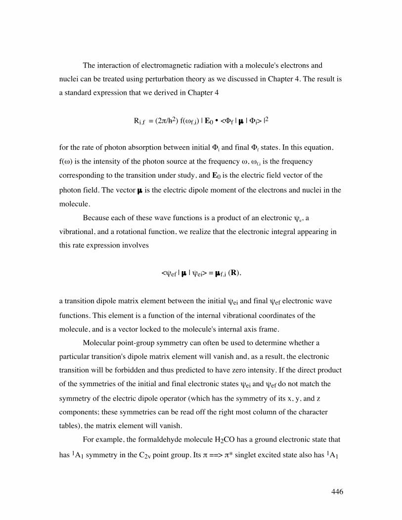
446

The interaction of electromagnetic radiation with a molecule's electrons and

nuclei can be treated using perturbation theory as we discussed in Chapter 4. The result is

a standard expression that we derived in Chapter 4

Ri,f = (2π/h2) f(ωf,i) | E0 • <Φf | µ | Φi> |2

for the rate of photon absorption between initial Φi and final Φf states. In this equation,

f(ω) is the intensity of the photon source at the frequency ω, ωf,i is the frequency

corresponding to the transition under study, and E0 is the electric field vector of the

photon field. The vector µ is the electric dipole moment of the electrons and nuclei in the

molecule.

Because each of these wave functions is a product of an electronic ψe, a

vibrational, and a rotational function, we realize that the electronic integral appearing in

this rate expression involves

<ψef | µ | ψei> = µ f,i (R),

a transition dipole matrix element between the initial ψei and final ψef electronic wave

functions. This element is a function of the internal vibrational coordinates of the

molecule, and is a vector locked to the molecule's internal axis frame.

Molecular point-group symmetry can often be used to determine whether a

particular transition's dipole matrix element will vanish and, as a result, the electronic

transition will be forbidden and thus predicted to have zero intensity. If the direct product

of the symmetries of the initial and final electronic states ψei and ψef do not match the

symmetry of the electric dipole operator (which has the symmetry of its x, y, and z

components; these symmetries can be read off the right most column of the character

tables), the matrix element will vanish.

For example, the formaldehyde molecule H2CO has a ground electronic state that

has 1A1 symmetry in the C2v point group. Its π ==> π* singlet excited state also has 1A1

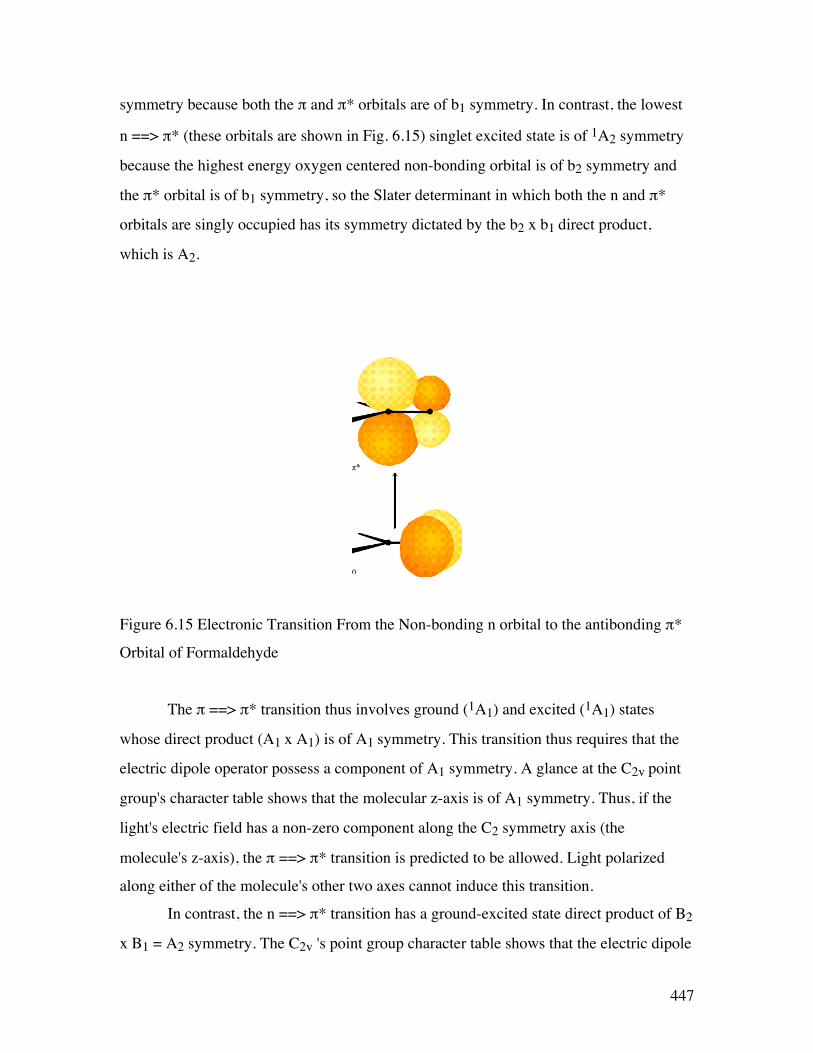
447

symmetry because both the π and π* orbitals are of b1 symmetry. In contrast, the lowest

n ==> π* (these orbitals are shown in Fig. 6.15) singlet excited state is of 1A2 symmetry

because the highest energy oxygen centered non-bonding orbital is of b2 symmetry and

the π* orbital is of b1 symmetry, so the Slater determinant in which both the n and π*

orbitals are singly occupied has its symmetry dictated by the b2 x b1 direct product,

which is A2.

Figure 6.15 Electronic Transition From the Non-bonding n orbital to the antibonding π*

Orbital of Formaldehyde

The π ==> π* transition thus involves ground (1A1) and excited (1A1) states

whose direct product (A1 x A1) is of A1 symmetry. This transition thus requires that the

electric dipole operator possess a component of A1 symmetry. A glance at the C2v point

group's character table shows that the molecular z-axis is of A1 symmetry. Thus, if the

light's electric field has a non-zero component along the C2 symmetry axis (the

molecule's z-axis), the π ==> π* transition is predicted to be allowed. Light polarized

along either of the molecule's other two axes cannot induce this transition.

In contrast, the n ==> π* transition has a ground-excited state direct product of B2

x B1 = A2 symmetry. The C2v 's point group character table shows that the electric dipole

448

operator (i.e., its x, y, and z components in the molecule-fixed frame) has no component

of A2 symmetry; thus, light of no electric field orientation can induce this n ==> π*

transition. We thus say that the n ==> π* transition is forbidden.

The above examples illustrate one of the most important applications of visible-

UV spectroscopy. The information gained in such experiments can be used to infer the

symmetries of the electronic states and hence of the orbitals occupied in these states. It is

in this manner that this kind of experiment probes electronic structures.

2. The Franck-Condon Factors

Beyond such electronic symmetry analysis, it is also possible to derive vibrational

selection rules for electronic transitions that are allowed. It is conventional to expand the

transition dipole matrix element µ f,i (R) in a power series about the equilibrium geometry

of the initial electronic state (since this geometry is characteristic of the molecular

structure prior to photon absorption and, because the photon absorption takes place

quickly, the nuclei don’t have time to move far from there):

µ f,i(R) = µ f,i(Re) + Σa ∂µ f,i/∂Ra (Ra - Ra,e) + ....

The first term in this expansion, when substituted into the integral over the vibrational

coordinates, gives µ f,i(Re) <χvf | χvi> , which has the form of the electronic transition

dipole multiplied by the overlap integral between the initial and final vibrational wave

functions. The µ f,i(Re) factor was discussed above; it is the electronic transition integral

evaluated at the equilibrium geometry of the absorbing state. Symmetry can often be used

to determine whether this integral vanishes, as a result of which the transition will be

forbidden.

The vibrational overlap integrals <χvf | χvi> do not necessarily vanish because

χvf and χvi are eigenfunctions of different vibrational Hamiltonians because they belong

to different Born-Oppenheimer energy surfaces. χvf is an eigenfunction whose potential

energy is the final electronic state's energy surface; χvi has the initial electronic state's

449

energy surface as its potential. The squares of these <χvf | χvi> integrals, which are what

eventually enter into the transition rate expression Ri,f = (2π/h2) f(ωf,i) | E0 • <Φf | µ |

Φi> |2, are called Franck-Condon factors. Their relative magnitudes play strong roles in

determining the relative intensities of various vibrational bands (i.e., series of peaks)

within a particular electronic transition's spectrum. In Fig. 6.16, I show two potential

energy curves and illustrate the kinds of absorption (and emission) transitions that can

occur when the two electronic states have significantly different geometries.

Figure 6.16 Absorption From One Initial State to One Final State Followed by Relaxation

and Then Emission From the Lowest State of the Upper Surface.

Whenever an electronic transition causes a large change in the geometry (bond

lengths or angles) of the molecule, the Franck-Condon factors tend to display the

characteristic broad progression shown in Fig. 6.17 when considered for one initial-state

vibrational level vi and various final-state vibrational levels vf:

450

vf= 0 1 2 3 4 5 6

|<χi|χf>|2

Final state vibrational Energy (Evf)

Figure 6.17 Broad Franck-Condon Progression Characteristic of Large Geometry Change

Notice that as one moves to higher vf values, the energy spacing between the states (Evf -

Evf-1) decreases; this, of course, reflects the anharmonicity in the excited-state vibrational

potential. For the above example, the transition to the vf = 2 state has the largest Franck-

Condon factor. This means that the overlap of the initial state's vibrational wave function

χvi is largest for the final state's χvf function with vf = 2.

As a qualitative rule of thumb, the larger the geometry difference between the

initial- and final- state potentials, the broader will be the Franck-Condon profile (as

shown in Fig. 6.17) and the larger the vf value for which this profile peaks. Differences in

harmonic frequencies between the two states can also broaden the Franck-Condon

profile.

If the initial and final states have very similar geometries and frequencies along

the mode that is excited when the particular electronic excitation is realized, the type of

Franck-Condon profile shown in Fig. 6.18 may result:

451

vf= 0 1 2 3 4 5 6

|<χi|χf>|2

Final state vibrational Energy (Evf)

Figure 6.18 Franck-Condon Profile Characteristic of Small Geometry Change

Another feature that is important to emphasize is the relation between absorption

and emission when the two states’ energy surfaces have different equilibrium geometries

or frequencies. Subsequent to photon absorption to form an excited electronic state but

prior to photon emission, the molecule can undergoe collisions with other nearby

molecules. This, of course, is especially true in condensed-phase experiments. These

collisions cause the excited molecule to lose some of its vibrational and rotational energy,

thereby relaxing it to lower levels on the excited electronic surface. This relaxation

process is illustrated in Fig. 6.19.

452

Figure 6.19 Absorption Followed by Relaxation to Lower Vibrational Levels of the

Upper State.

Subsequently, the electronically excited molecule can undergo photon emission (also

called fluorescence) to return to its ground electronic state as shown in Fig. 6.20.

Figure 6.20 Fluorescence From Lower Levels of the Upper Surface

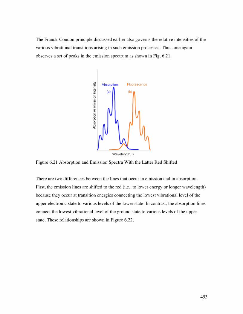
453

The Franck-Condon principle discussed earlier also governs the relative intensities of the

various vibrational transitions arising in such emission processes. Thus, one again

observes a set of peaks in the emission spectrum as shown in Fig. 6.21.

Figure 6.21 Absorption and Emission Spectra With the Latter Red Shifted

There are two differences between the lines that occur in emission and in absorption.

First, the emission lines are shifted to the red (i.e., to lower energy or longer wavelength)

because they occur at transition energies connecting the lowest vibrational level of the

upper electronic state to various levels of the lower state. In contrast, the absorption lines

connect the lowest vibrational level of the ground state to various levels of the upper

state. These relationships are shown in Figure 6.22.

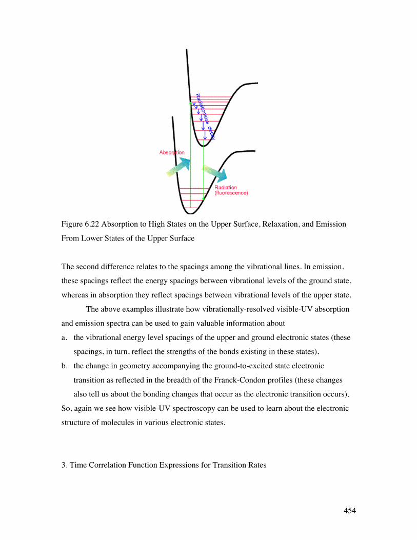
454

Figure 6.22 Absorption to High States on the Upper Surface, Relaxation, and Emission

From Lower States of the Upper Surface

The second difference relates to the spacings among the vibrational lines. In emission,

these spacings reflect the energy spacings between vibrational levels of the ground state,

whereas in absorption they reflect spacings between vibrational levels of the upper state.

The above examples illustrate how vibrationally-resolved visible-UV absorption

and emission spectra can be used to gain valuable information about

a. the vibrational energy level spacings of the upper and ground electronic states (these

spacings, in turn, reflect the strengths of the bonds existing in these states),

b. the change in geometry accompanying the ground-to-excited state electronic

transition as reflected in the breadth of the Franck-Condon profiles (these changes

also tell us about the bonding changes that occur as the electronic transition occurs).

So, again we see how visible-UV spectroscopy can be used to learn about the electronic

structure of molecules in various electronic states.

3. Time Correlation Function Expressions for Transition Rates

455

The above so-called golden-rule expression for the rates of photon-induced

transitions are written in terms of the initial and final electronic/vibrational/rotational

states of the molecule. There are situations in which these states simply cannot be reliably

known. For example, the higher vibrational states of a large polyatomic molecule or the

states of a molecule that strongly interacts with surrounding solvent molecules are such

cases. In such circumstances, it is possible to recast the golden rule formula into a form

that is more amenable to introducing specific physical models that lead to additional

insights.

Specifically, by using so-called equilibrium averaged time correlation functions, it

is possible to obtain rate expressions appropriate to a large number of molecules that exist

in a distribution of initial states (e.g., for molecules that occupy many possible rotational

and perhaps several vibrational levels at room temperature). As we will soon see, taking

this route to expressing spectroscopic transition rates also allows us to avoid having to

know each vibrational-rotational wave function of the two electronic states involved; as

noted above, this is especially useful for large molecules or molecules in condensed

media where such knowledge is likely not available.

To begin re-expressing the spectroscopic transition rates, the expression obtained

earlier

Ri,f = (2π/h2) f(ωf,i) | E0 • <Φf | µ | Φi> |2 ,

appropriate to transitions between a particular initial state Φi and a specific final state Φf,

is rewritten as

Ri,f = (2π/h2)

€

f (ω) |E0• <Φ f |µ |Φi >|2 δ(ω f ,i−ω)dω∫ .

Here, the δ(ωf,i - ω) function is used to specifically enforce the resonance condition

which states that the photons' frequency ω must be resonant with the transition frequency

ωf,i . The following integral identity can be used to replace the δ-function:

456

δ(ωf,i - ω) =

€

12π

exp[i(ω f ,i−ω)t]dt

−∞

∞

∫

by a form that is more amenable to further development. Then, the state-to-state rate of

transition becomes:

Ri,f = (1/h2)

€

f (ω) |E0• <Φ f |µ |Φi >|2 exp[i(ω f ,i−ω)t]dtdω

−∞

∞

∫∫ .

If this expression is then multiplied by the equilibrium probability ρi that the

molecule is found in the state Φi and summed over all such initial states and summed

over all final states Φf that can be reached from Φi with photons of energy h ω, the

equilibrium averaged rate of photon absorption by the molecular sample is obtained:

Req.ave. = (1/h2)Σf,i ρi

€

f (ω) |E0• <Φ f |µ |Φi >|2 exp[i(ω f ,i−ω)t]dt

−∞

∞

∫ δω∫ .

This expression is appropriate for an ensemble of molecules that can be in various initial

states Φi with probabilities ρi. The corresponding result for transitions that originate in a

particular state (Φi) but end up in any of the allowed (by energy and selection rules) final

states reads:

Ri = (1/h2)Σf ρi

€

f (ω) |E0• <Φ f |µ |Φi >|2 exp[i(ω f ,i−ω)t]dt

−∞

∞

∫ δω∫ .

As we discuss in Chapter 7, for an ensemble in which the number of molecules, the

temperature T, and the system volume are specified, ρi takes the form:

ρi = gi exp(-Ei0/kT)/Q

457

where Q is the partition function of the molecules and gi is the degeneracy of the state Φi

whose energy is Ei0. If you are unfamiliar with partition functions and do not want to

simply trust me in the analysis of time correlation functions that we am about to

undertake, I suggest you interrupt your study of Chapter 6 and read up through Section

7.1.3 of Chapter 7 at this time.

In the above expression for Req.ave., a double sum occurs. Writing out the

elements that appear in this sum in detail, one finds:

Σi, f ρi E0 • <Φi | µ | Φf> E0 • <Φf | µ | Φi> exp[i(ωf,i)t].

In situations in which one is interested in developing an expression for the intensity

arising from transitions to all allowed final states, the sum over the final states can be

carried out explicitly by first writing

<Φf | µ | Φi> exp[i(ωf,i)t] = <Φf |exp(iHt/h) µ exp(-iHt/h)| Φi>

and then using the fact that the set of states {Φk} are complete and hence obey

Σk |Φk><Φk| = 1.

The result of using these identities as well as the Heisenberg definition of the time-

dependence of the dipole operator

µ(t) = exp(iHt/h) µ exp(-iHt/h),

is:

Σi ρi <Φi | E0 • µ E0 • µ (t) | Φi> .

458

In this form, one says that the time dependence has been reduce to that of an equilibrium

averaged (i.e., as reflected in the Σi ρi <Φi | | Φi> expression) time correlation function

involving the component of the dipole operator along the external electric field at t = 0,

( E0 • µ ) and this component at a different time t, (E0 • µ (t)).

If ωf,i is positive (i.e., in the photon absorption case), the above expression will

yield a non-zero contribution when multiplied by exp(-i ωt) and integrated over positive

ω- values. If ωf,i is negative (as for stimulated photon emission), this expression will

contribute, when multiplied by exp(-i ωt), for negative ω-values. In the latter situation, ρi

is the equilibrium probability of finding the molecule in the (excited) state from which

emission will occur; this probability can be related to that of the lower state ρf by

ρexcited = ρlower exp[ - (E0excited - E0lower)/kT ]

= ρlower exp[ - hω/kT ].

The absorption and emission cases can be combined into a single expression for

the net rate of photon absorption by recognizing that the latter process leads to photon

production, and thus must be entered with a negative sign. The resultant expression for

the net rate of decrease of photons is:

Req.ave.net = (1/h2) Σi ρi

€

f (ω) <Φi | (E0 •µ)E0 •µ(t) |Φi >∫∫ (1 - exp(- h ω/kT) ) exp(-iωt) dω dt.

It is convention to introduce the so-called line shape function I (ω):

I (ω) = Σi ρi

€

<Φi | (E0 •µ)E0 •µ(t) |Φi >∫ exp(-iωt) dt

459

in terms of which the net photon absorption rate is

Req.ave.net = (1/h2) (1 - exp(- h ω/kT) )

€

f (ω)I(ω)dω∫ .

The function

C (t) = Σi ρi <Φi | (E0 • µ ) E0 • µ (t) | Φi>

is called the equilibrium averaged time correlation function of the component of the

electric dipole operator along the direction of the external electric field E0. Its Fourier

transform is I (ω), the spectral line shape function. The convolution of I (ω) with the light

source's f (ω) function, multiplied by (1 - exp(-h ω/kT) ), the correction for stimulated

photon emission, gives the net rate of photon absorption.

Although the correlation function expression for the photon absorption rate is

equivalent to the state-to-state expression from which it was derived, we notice that

a. C(t) does not contain explicit reference to the final-state wave functions Φf; instead,

b. C(t) requires us to describe how the dipole operator changes with time.

That is, in the time correlation framework, one is allowed to use models of the time

evolution of the system to describe the spectra. This is especially appealing for large

complex molecules and molecules in condensed media because, for such systems, it

would be hopeless to attempt to find the final-state wave functions, but it may be

reasonable (albeit challenging) to model the system’s time evolution. Prof. Eric Heller at

Harvard has pioneered the use of time-domain methods for treating molecular

spectroscopy; his web site (http://monsoon.harvard.edu/) offers access to further

information and insight into this subject.

It turns out that a very wide variety of spectroscopic and thermodynamic

properties (e.g., light scattering intensities, diffusion coefficients, and thermal

conductivity) can be expressed in terms of molecular time correlation functions. The text

Statistical Mechanics, D. A. McQuarrie, Harper and Row, New York (1977) has a good

460

treatment of many of these cases. Let’s now examine how such time evolution issues are

used within the correlation function framework for the specific photon absorption case.

4. Line Broadening Mechanisms

If the rotational motion of the system’s molecules is assumed to be entirely

unhindered (e.g., by any environment or by collisions with other molecules), it is

appropriate to express the time dependence of each of the dipole time correlation

functions listed above in terms of a free rotation model. For example, when dealing with

diatomic molecules, the electronic-vibrational-rotational C(t) appropriate to a specific

electronic-vibrational transition becomes:

C(t) = (qr qv qe qt)-1 ΣJ (2J+1) exp(- h2J(J+1)/(8π2IkT)) exp(- hνvibvi /kT)

gie <φJ | E0 • µ i,f(Re) E0 • µ i,f(Re,t) |φJ> |<χiv | χfv>|2

exp(i [hνvib] t + iΔEi,f t/h).

Here,

qr = (8π2IkT/h2)

is the rotational partition function (I being the molecule's moment of inertia

I = µRe2, and h2J(J+1)/(8π2I) being the molecule's rotational energy for the state with

quantum number J and degeneracy 2J+1),

qv = exp(-hνvib/2kT) (1-exp(-hνvib/kT))-1

is the vibrational partition function (νvib being the vibrational frequency), gie is the

degeneracy of the initial electronic state,

461

qt = (2πmkT/h2)3/2 V

is the translational partition function for the molecules of mass m moving in volume V,

and ΔEi,f is the adiabatic electronic energy spacing. The origins of such partition

functions are treated in Chapter 7 of this text.

The functions <φJ | E0 • µ i,f(Re) E0 • µ i,f(Re,t) |φJ> describe the time evolution of

the electronic transition dipole vector for the rotational state J. In a free-rotation model,

this function is taken to be of the form:

<φJ | E0 • µ i,f(Re) E0 • µ i,f(Re,t) |φJ>

= <φJ | E0 • µ i,f(Re) E0 • µ i,f(Re) |φJ> Cos(ωJt)

where ωJ is the rotational frequency (in cycles per second) for rotation of the molecule in

the state labeled by J. This oscillatory time dependence, combined with the exp(i [hνvib] t

+ iΔEi,f t/h) time dependence arising from the electronic and vibrational factors, produce,

when this C(t) function is Fourier transformed to generate I(ω), a series of δ-function

peaks. The intensities of these peaks are governed by the quantities

(qr qv qe qt)-1 ΣJ (2J+1) exp(- h2J(J+1)/(8π2IkT)) exp(- hνvibvi /kT) gie,

Boltzmann population factors, as well as by the |<χiv | χfv>|2 Franck-Condon factors and

the <φJ | E0 • µ i,f(Re) E0 • µ i,f(Re,0) |φJ> terms.

This same analysis can be applied to the pure rotation and vibration-rotation C(t)

time dependences with analogous results. In the former, δ-function peaks are predicted to

occur at

ω = ± ωJ

462

and in the latter at

ω = ωfv,iv ± ωJ ;

with the intensities governed by the time independent factors in the corresponding

expressions for C(t).

In experimental measurements, such sharp δ-function peaks are, of course, not

observed. Even when very narrow bandwidth laser light sources are used (i.e., for which

f(ω) is an extremely narrowly peaked function), spectral lines are found to possess finite

widths. Let us now discuss several sources of line broadening, some of which will relate

to deviations from the "unhindered" rotational motion model introduced above.

a. Doppler Broadening

In the above expressions for C(t), the averaging over initial rotational, vibrational,

and electronic states is explicitly shown. There is also an average over the translational

motion implicit in all of these expressions. Its role has not (yet) been emphasized because

the molecular energy levels, whose spacings yield the characteristic frequencies at which

light can be absorbed or emitted, do not depend on translational motion. However, the

frequency of the electromagnetic field experienced by moving molecules does depend on

the velocities of the molecules, so this issue must now be addressed.

Elementary physics classes express the so-called Doppler shift of a wave's

frequency induced by relative movement of the light source and the molecule as follows:

ωobserved = ωnominal (1 + vz/c)-1 ≈ ωnominal (1 - vz/c + ...).

Here, ωnominal is the frequency of the unmoving light source seen by unmoving

molecules, vz is the velocity of relative motion of the light source and molecules, c is the

speed of light, and ωobserved is the Doppler-shifted frequency (i.e., the frequency seen by

the molecules). The second identity is obtained by expanding, in a power series, the (1 +

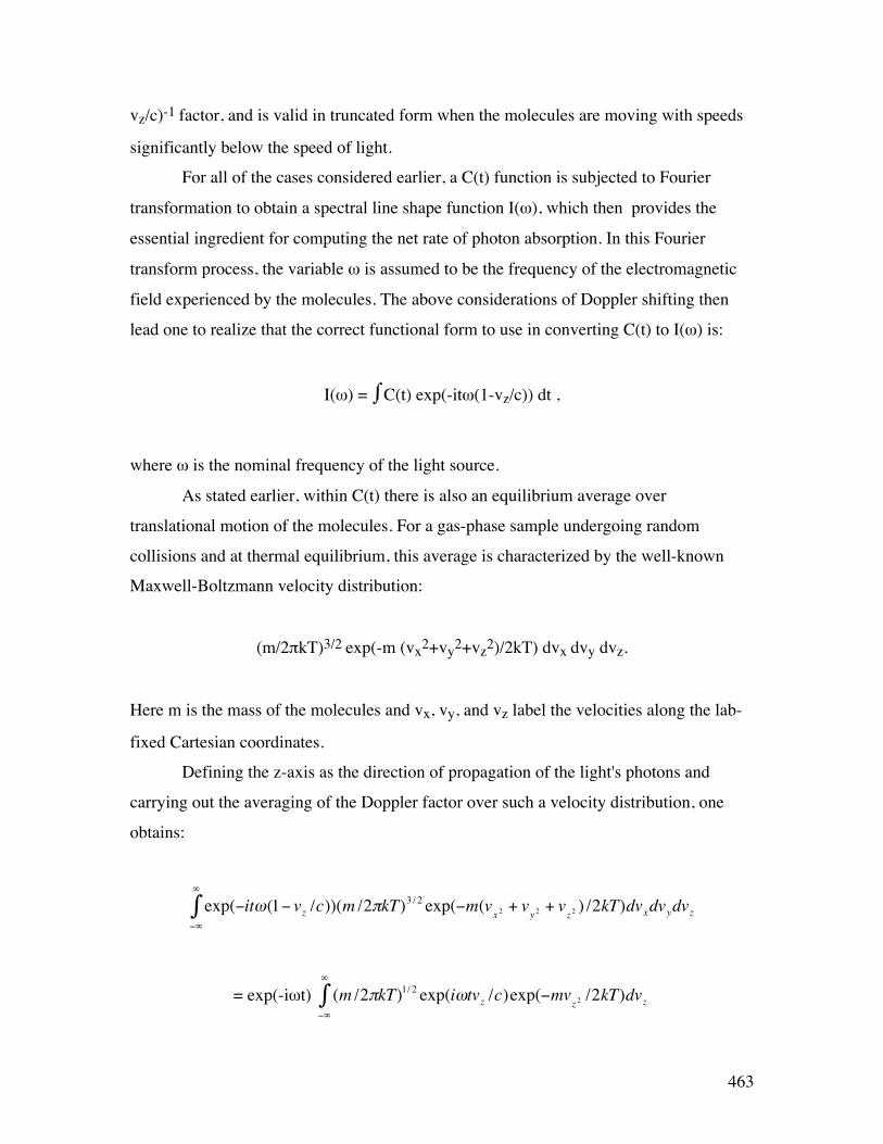
463

vz/c)-1 factor, and is valid in truncated form when the molecules are moving with speeds

significantly below the speed of light.

For all of the cases considered earlier, a C(t) function is subjected to Fourier

transformation to obtain a spectral line shape function I(ω), which then provides the

essential ingredient for computing the net rate of photon absorption. In this Fourier

transform process, the variable ω is assumed to be the frequency of the electromagnetic

field experienced by the molecules. The above considerations of Doppler shifting then

lead one to realize that the correct functional form to use in converting C(t) to I(ω) is:

I(ω) = ⌡⌠C(t) exp(-itω(1-vz/c)) dt ,

where ω is the nominal frequency of the light source.

As stated earlier, within C(t) there is also an equilibrium average over

translational motion of the molecules. For a gas-phase sample undergoing random

collisions and at thermal equilibrium, this average is characterized by the well-known

Maxwell-Boltzmann velocity distribution:

(m/2πkT)3/2 exp(-m (vx2+vy2+vz2)/2kT) dvx dvy dvz.

Here m is the mass of the molecules and vx, vy, and vz label the velocities along the lab-

fixed Cartesian coordinates.

Defining the z-axis as the direction of propagation of the light's photons and

carrying out the averaging of the Doppler factor over such a velocity distribution, one

obtains:

€

exp(−itω(1− vz /c))(m /2πkT)3 / 2 exp(−m(v

x 2+ v

y 2+ v

z 2) /2kT)dvxdvydvz

−∞

∞

∫

= exp(-iωt)

€

(m /2πkT)1/ 2 exp(iωtvz /c)exp(−mvz 2 /2kT)dvz−∞

∞

∫

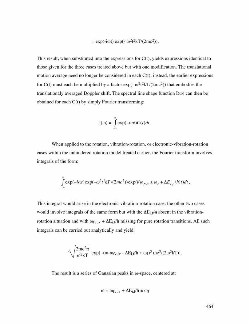
464

= exp(-iωt) exp(- ω2t2kT/(2mc2)).

This result, when substituted into the expressions for C(t), yields expressions identical to

those given for the three cases treated above but with one modification. The translational

motion average need no longer be considered in each C(t); instead, the earlier expressions

for C(t) must each be multiplied by a factor exp(- ω2t2kT/(2mc2)) that embodies the

translationaly averaged Doppler shift. The spectral line shape function I(ω) can then be

obtained for each C(t) by simply Fourier transforming:

I(ω) =

€

exp(−iωt)C(t)dt−∞

∞

∫ .

When applied to the rotation, vibration-rotation, or electronic-vibration-rotation

cases within the unhindered rotation model treated earlier, the Fourier transform involves

integrals of the form:

€

exp(−iωt)exp(−ω 2t 2kT /(2mc 2))exp(i(ω fv,iv ±ωJ + ΔEi, f /)t)dt−∞

∞

∫ .

This integral would arise in the electronic-vibration-rotation case; the other two cases

would involve integrals of the same form but with the ΔEi,f/h absent in the vibration-

rotation situation and with ωfv,iv + ΔEi,f/h missing for pure rotation transitions. All such

integrals can be carried out analytically and yield:

2mc2πω2kT exp[ -(ω-ωfv,iv - ΔEi,f/h ± ωJ)2 mc2/(2ω2kT)].

The result is a series of Gaussian peaks in ω-space, centered at:

ω = ωfv,iv + ΔEi,f/h ± ωJ

465

with widths (σ) determined by

σ2 = ω2kT/(mc2),

given the temperature T and the mass of the molecules m. The hotter the sample, the

faster the molecules are moving on average, and the broader is the distribution of Doppler

shifted frequencies experienced by these molecules. The net result then of the Doppler

effect is to produce a line shape function that is similar to the unhindered rotation model's

series of δ-functions but with each δ-function peak broadened into a Gaussian shape.

If spectra can be obtained to accuracy sufficient to determine the Doppler width

of the spectral lines, such knowledge can be used to estimate the temperature of the

system. This can be useful when dealing with systems that cannot be subjected to

alternative temperature measurements. For example, the temperatures of stars can be

estimated (if their velocity relative to the earth is known) by determining the Doppler

shifts of emission lines from them. Alternatively, the relative speed of a star from the

earth may be determined if its temperature is known. As another example, the

temperature of hot gases produced in an explosion can be probed by measuring Doppler

widths of absorption or emission lines arising from molecules in these gases.

b. Pressure Broadening

To include the effects of collisions on the rotational motion part of any of the

above C(t) functions, one must introduce a model for how such collisions change the

dipole-related vectors that enter into C(t). The most elementary model used to address

collisions applies to gaseous samples which are assumed to undergo unhindered

rotational motion until struck by another molecule at which time a kick is applied to the

dipole vector and after which the molecule returns to its unhindered rotational movement.

The effects of such infrequent collision-induced kicks are treated within the so-

called pressure broadening (sometimes called collisional broadening) model by

modifying the free-rotation correlation function through the introduction of an

exponential damping factor exp( -|t|/τ):

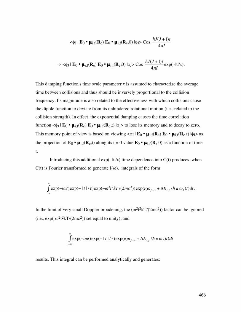
466

<φJ | E0 • µ i,f(Re) E0 • µ i,f(Re,0) |φJ> Cos

€

hJ(J +1)t4πI

⇒ <φJ | E0 • µ i,f(Re) E0 • µ i,f(Re,0) |φJ> Cos

€

hJ(J +1)t4πI

exp( -|t|/τ).

This damping function's time scale parameter τ is assumed to characterize the average

time between collisions and thus should be inversely proportional to the collision

frequency. Its magnitude is also related to the effectiveness with which collisions cause

the dipole function to deviate from its unhindered rotational motion (i.e., related to the

collision strength). In effect, the exponential damping causes the time correlation

function <φJ | E0 • µ i,f(Re) E0 • µ i,f(Re,t) |φJ> to lose its memory and to decay to zero.

This memory point of view is based on viewing <φJ | E0 • µ i,f(Re) E0 • µ i,f(Re,t) |φJ> as

the projection of E0 • µ i,f(Re,t) along its t = 0 value E0 • µ i,f(Re,0) as a function of time

t.

Introducing this additional exp( -|t|/τ) time dependence into C(t) produces, when

C(t) is Fourier transformed to generate I(ω), integrals of the form

€

exp(−iωt)exp(− | t | /τ)exp(−ω 2t 2kT /(2mc 2))exp(i(ω fv,iv + ΔEi, f / ±ωJ )t)dt−∞

∞

∫ .

In the limit of very small Doppler broadening, the (ω2t2kT/(2mc2)) factor can be ignored

(i.e., exp(-ω2t2kT/(2mc2)) set equal to unity), and

€

exp(−iωt)exp(− | t | /τ)exp(i(ω fv,iv + ΔEi, f / ±ωJ )t)dt−∞

∞

∫

results. This integral can be performed analytically and generates:

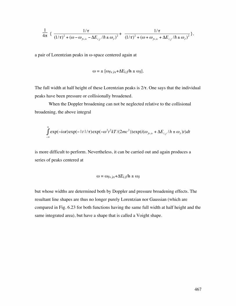
467

14π {

€

1/τ(1/τ )2 + (ω −ω fv,iv −ΔEi, f / ±ωJ )

2 +

€

1/τ(1/τ )2 + (ω +ω fv,iv + ΔEi, f / ±ωJ )

2 },

a pair of Lorentzian peaks in ω-space centered again at

ω = ± [ωfv,iv+ΔEi,f/h ± ωJ].

The full width at half height of these Lorentzian peaks is 2/τ. One says that the individual

peaks have been pressure or collisionally broadened.

When the Doppler broadening can not be neglected relative to the collisional

broadening, the above integral

€

exp(−iωt)exp(− | t | /τ)exp(−ω 2t 2kT /(2mc 2))exp(i(ω fv,iv + ΔEi, f /h ±ωJ )t)dt−∞

∞

∫

is more difficult to perform. Nevertheless, it can be carried out and again produces a

series of peaks centered at

ω = ωfv,iv+ΔEi,f/h ± ωJ

but whose widths are determined both by Doppler and pressure broadening effects. The

resultant line shapes are thus no longer purely Lorentzian nor Gaussian (which are

compared in Fig. 6.23 for both functions having the same full width at half height and the

same integrated area), but have a shape that is called a Voight shape.

468

Inte

nsity

ω

Gaussian(Doppler)

Lorentzian

Figure 6.23 Typical Forms of Gaussian and Lorentzian Peaks having identical widths and

areas.

Experimental measurements of line widths that allow one to extract widths

originating from collisional broadening provide information (through τ) on the frequency

of collisions and the strength of these collisions. By determining τ at a series of gas

densities, one can separate the collision-frequency dependence and determine the strength

of the individual collisions (meaning how effective each collision is in reorienting the

molecule’s dipole vector).

c. Rotational Diffusion Broadening

Molecules in liquids and very dense gases undergo such frequent collisions with

the other molecules that the mean time between collisions is short compared to the

rotational period for their unhindered rotation. As a result, the time dependence of the

dipole-related correlation functions can no longer be modeled in terms of free rotation

that is interrupted by (infrequent) collisions and Doppler shifted. Instead, a model that

describes the incessant buffeting of the molecule's dipole by surrounding molecules

becomes appropriate. For liquid samples in which these frequent collisions cause the

dipole to undergo angular motions that cover all angles (i.e., in contrast to a frozen glass

or solid in which the molecule's dipole would undergo strongly perturbed pendular

469

motion about some favored orientation), the so-called rotational diffusion model is often

used.

In this picture, the rotation-dependent part of C(t) is expressed as:

<φJ | E0 • µ i,f(Re) E0 • µ i,f(Re,t) |φJ>

= <φJ | E0 • µ i,f(Re) E0 • µ i,f(Re,0) |φJ> exp( -2Drot|t|),

where Drot is the rotational diffusion constant whose magnitude details the time

decay in the averaged value of E0 • µ i,f(Re,t) at time t with respect to its value at time t =

0; the larger Drot, the faster is this decay. As with pressure broadening, this exponential

time dependence, when subjected to Fourier transformation, yields:

€

exp(−iωt)exp(−2Drot | t |)exp(−ω2t 2kT /(2mc 2))exp(i(ω fv,iv + ΔEi, f / ±ωJ )t)dt

−∞

∞

∫ .

Again, in the limit of very small Doppler broadening, the (ω2t2kT/(2mc2)) factor can be

ignored (i.e., exp(-ω2t2kT/(2mc2)) set equal to unity), and

€

exp(−iωt)exp(−2Drot | t |)exp(i(ω fv,iv + ΔEi, f / ±ωJ )t)dt−∞

∞

∫

results. This integral can be evaluated analytically and generates:

1

4π {

€

2Drot

(2Drot )2 + (ω −ω fv,iv −ΔEi, f / ±ωJ )

2

+

€

2Drot

(2Drot )2 + (ω +ω fv,iv + ΔEi, f / ±ωJ )

2 },

a pair of Lorentzian peaks in ω-space centered again at

470

ω = ±[ωfv,iv+ΔEi,f/h ± ωJ].

The full width at half height of these Lorentzian peaks is 4Drot. In this case, one says that

the individual peaks have been broadened via rotational diffusion. In such cases,

experimental measurement of line widths yield valuable information about how fast the

molecule is rotationally diffusing in its condensed environment.

d. Lifetime or Heisenberg Homogeneous Broadening

Whenever the absorbing species undergoes one or more processes that depletes its

numbers, we say that it has a finite lifetime. For example, a species that undergoes

unimolecular dissociation has a finite lifetime, as does an excited state of a molecule that

decays by spontaneous emission of a photon. Any process that depletes the absorbing

species contributes another source of time dependence for the dipole time correlation

functions C(t) discussed above. This time dependence is usually modeled by appending,

in a multiplicative manner, a factor exp(-|t|/τ). This, in turn modifies the line shape

function I(ω) in a manner much like that discussed when treating the rotational diffusion

case:

€

exp(−iωt)exp(− | t | /τ)exp(−ω 2t 2kT /(2mc 2))exp(i(ω fv,iv + ΔEi, f / ±ωJ )t)dt−∞

∞

∫ .

Not surprisingly, when the Doppler contribution is small, one obtains:

1

4π {

€

1/τ(1/τ )2 + (ω −ω fv,iv −ΔEi, f / ±ωJ )

2

+

€

1/τ(1/τ )2 + (ω +ω fv,iv + ΔEi, f / ±ωJ )

2 }.

471

In these Lorentzian lines, the parameter τ describes the kinetic decay lifetime of the

molecule. One says that the spectral lines have been lifetime or Heisenberg broadened by

an amount proportional to 1/τ. The latter terminology arises because the finite lifetime of

the molecular states can be viewed as producing, via the Heisenberg uncertainty relation

ΔEΔt > h, states whose energy is uncertain to within an amount ΔE.

e. Site Inhomogeneous Broadening

Among the above line broadening mechanisms, the pressure, rotational diffusion,

and lifetime broadenings are all of the homogeneous variety. This means that each and

every molecule in the sample is affected in exactly the same manner by the broadening

process. For example, one does not find some molecules with short lifetimes and others

with long lifetimes in the Heisenberg case; the entire ensemble of molecules is

characterized by a single lifetime.

In contrast, Doppler broadening is inhomogeneous in nature because each

molecule experiences a broadening that is characteristic of its particular velocity vz. That

is, the fast molecules have their lines broadened more than do the slower molecules.

Another important example of inhomogeneous broadening is provided by so-called site

broadening. Molecules imbedded in a liquid, solid, or glass do not, at the instant of their

photon absorption, all experience exactly the same interactions with their surroundings.

The distribution of instantaneous solvation environments may be rather narrow (e.g., in a

highly ordered solid matrix) or quite broad (e.g., in a liquid at high temperature or in a

super-critical liquid). Different environments produce different energy level splittings ω

= ωfv,iv+ΔEi,f/h ± ωJ (because the initial and final states are solvated differently by the

surroundings) and thus different frequencies at which photon absorption can occur. The

distribution of energy level splittings causes the sample to absorb at a range of

frequencies as illustrated in Fig. 6.24 where homogeneous and inhomogeneous line

shapes are compared.

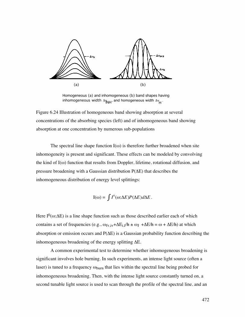
472

(a) (b)

Homogeneous (a) and inhomogeneous (b) band shapes having inhomogeneous width Δν , and homogeneous width Δν .INH H

Figure 6.24 Illustration of homogeneous band showing absorption at several

concentrations of the absorbing species (left) and of inhomogeneous band showing

absorption at one concentration by numerous sub-populations

The spectral line shape function I(ω) is therefore further broadened when site

inhomogeneity is present and significant. These effects can be modeled by convolving

the kind of I(ω) function that results from Doppler, lifetime, rotational diffusion, and

pressure broadening with a Gaussian distribution P(ΔE) that describes the

inhomogeneous distribution of energy level splittings:

I(ω) =

€

I0(ω;ΔE)∫ P(ΔE)dΔE .

Here I0(ω;ΔE) is a line shape function such as those described earlier each of which

contains a set of frequencies (e.g., ωfv,iv+ΔEi,f/h ± ωJ +ΔE/h = ω + ΔE/h) at which

absorption or emission occurs and P(ΔE) is a Gaussian probability function describing the

inhomogeneous broadening of the energy splitting ΔE.

A common experimental test to determine whether inhomogeneous broadening is

significant involves hole burning. In such experiments, an intense light source (often a

laser) is tuned to a frequency ωburn that lies within the spectral line being probed for

inhomogeneous broadening. Then, with the intense light source constantly turned on, a

second tunable light source is used to scan through the profile of the spectral line, and an

473

absorption spectrum is recorded. Given an absorption profile as shown in Fig. 6.25 in the

absence of the intense burning light source:

ω

Intensity

Figure 6.25 Absorption Profile in the Absence of Hole Burning

one expects to see a profile such as that shown in Fig. 6.26 if inhomogeneous broadening

is operative.

ω

Intensity

Figure 6.26 Absorption Profile With Laser Turned On to Burn a Hole

The interpretation of the change in the absorption profile caused by the bright

light source proceeds as follows:

(i) In the ensemble of molecules contained in the sample, some molecules will absorb at

or near the frequency of the bright light source ωburn; other molecules (those whose

474

environments do not produce energy level splittings that match ωburn) will not absorb at

this frequency.

(ii) Those molecules that do absorb at ωburn will have their transition saturated by the

intense light source, thereby rendering this frequency region of the line profile

transparent to further absorption.

(iii) When the probe light source is scanned over the line profile, it will induce

absorptions for those molecules whose local environments did not allow them to be

saturated by the ωburn light. The absorption profile recorded by this probe light source's

detector thus will match that of the original line profile, until

(iv) the probe light source's frequency matches ωburn, upon which no absorption of the

probe source's photons will be recorded because molecules that absorb in this frequency

regime have had their transition saturated.

(v) Hence, a hole will appear in the absorption spectrum recorded by the probe light

source's detector in the region of ωburn.

Unfortunately, the technique of hole burning does not provide a fully reliable

method for identifying inhomogeneously broadened lines. If a hole is observed in such a

burning experiment, this provides ample evidence, but if one is not seen, the result is not

definitive. In the latter case, the transition may not be strong enough (i.e., may not have a

large enough rate of photon absorption) for the intense light source to saturate the

transition to the extent needed to form a hole.

6.2.2 Photoelectron Spectroscopy

Photoelectron spectroscopy (PES) is a special kind of electronic spectroscopy. It

uses visible or UV light to excite a molecule or ion to a final state in which an electron is

ejected. In effect, it induces transitions to final states in which an electron has been

promoted to an unbound so-called continuum orbital. Most PES experiments are carried

out using a fixed-frequency light source (usually a laser). This source’s photons, when

absorbed, eject electrons whose intensity and kinetic energies KE are then measured.

Subtracting the electrons’ KE from the photon’s energy hν gives the binding energy BE

of the electron:

475

BE = hν - KE.

If the sample subjected to the PES experiment has molecules in a variety of initial states

(e.g., two electronic states or various vibrational-rotational levels of the ground electronic

state) having various binding energies BEk, one will observe a series of peaks

corresponding to electrons ejected with a variety of kinetic energies KEk as Fig. 6.27

illustrates and as the energy-balance condition requires:

BEk = hν - KEk.

The peak of electrons detected with the highest kinetic energy came from the highest-

lying state of the parent, while those with low kinetic energy came from the lowest-

energy state of the parent.

Figure 6.27 Photoelectron spectrum showing absorption from two states of the parent

476

By examining the spacings between these peaks, one learns about the spacings between

the energy levels of the parent species that has been subjected to electron loss.

Alternatively, if the parent species exists primarily in its lowest state but the

daughter species produced when an electron is removed from the parent has excited

(electronic, vibration-rotation) states that can be accessed, one can observe a different

progression of peaks. In this case, the electrons with highest kinetic energy arise from

transitions leading to the lowest-energy state of the daughter as Fig. 6.28 illustrates. In

that figure, the lower energy surface belongs to the parent and the upper curve to the

daughter.

◆◆◆◆◆◆◆◆◆◆◆◆◆◆◆◆◆◆◆◆◆◆◆◆◆◆◆◆◆◆◆◆

◆◆◆◆◆◆◆◆◆◆◆◆◆◆◆◆◆◆◆◆◆◆◆◆◆◆◆◆◆◆◆◆◆◆◆◆◆◆◆◆◆◆◆◆◆◆◆◆◆◆◆◆◆◆◆◆◆◆◆◆◆◆◆

◆◆◆◆◆◆◆◆◆◆◆◆◆

◆◆◆◆◆

*********************************

************************************************************************

********

0

5000

10000

15000

20000

25000

30000

E in

cm

-1

R in Angstroms

DetachingLight Source

Kinetic Energies of Detached Electrons

Figure 6.28 Photoelectron events showing detachment from one state of the parent to

several states of the daughter.

An example of experimental photodetachment data is provided in Fig. 6.29 showing the

intensity of electrons detected when Cu2- anion loses an electron vs. the kinetic energy of

the ejected electrons.

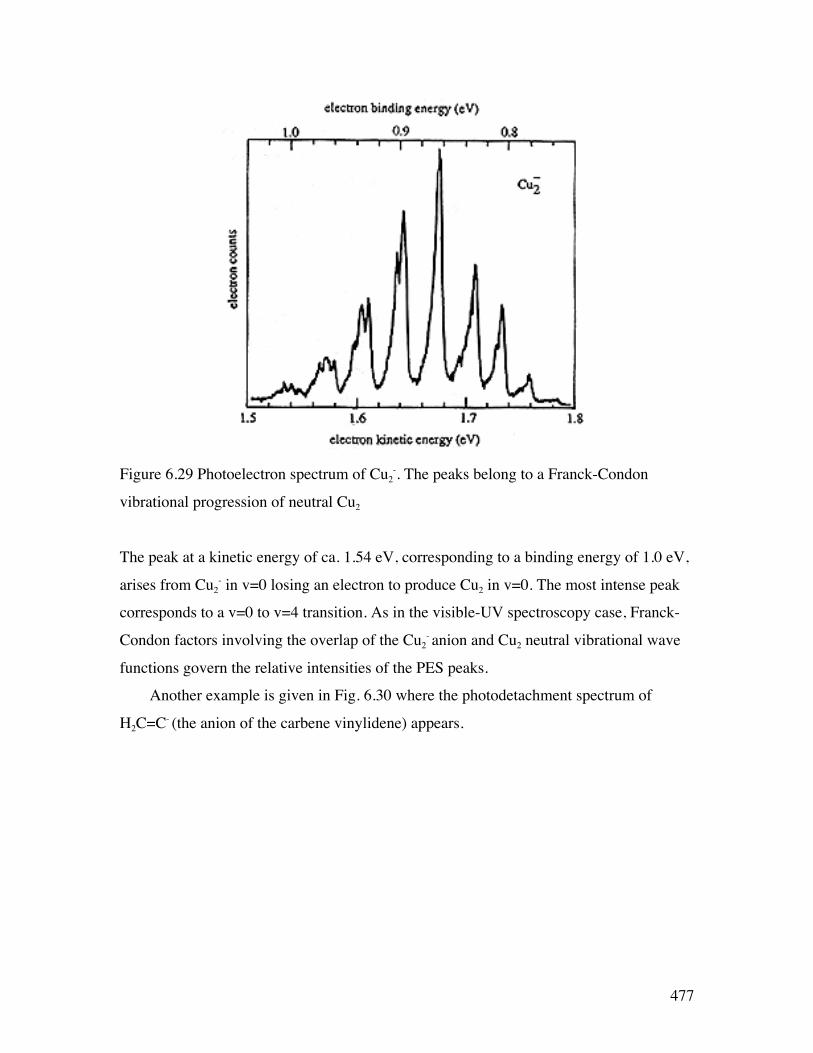
477

Figure 6.29 Photoelectron spectrum of Cu2

-. The peaks belong to a Franck-Condon

vibrational progression of neutral Cu2

The peak at a kinetic energy of ca. 1.54 eV, corresponding to a binding energy of 1.0 eV,

arises from Cu2- in v=0 losing an electron to produce Cu2 in v=0. The most intense peak

corresponds to a v=0 to v=4 transition. As in the visible-UV spectroscopy case, Franck-

Condon factors involving the overlap of the Cu2- anion and Cu2 neutral vibrational wave

functions govern the relative intensities of the PES peaks.

Another example is given in Fig. 6.30 where the photodetachment spectrum of

H2C=C- (the anion of the carbene vinylidene) appears.

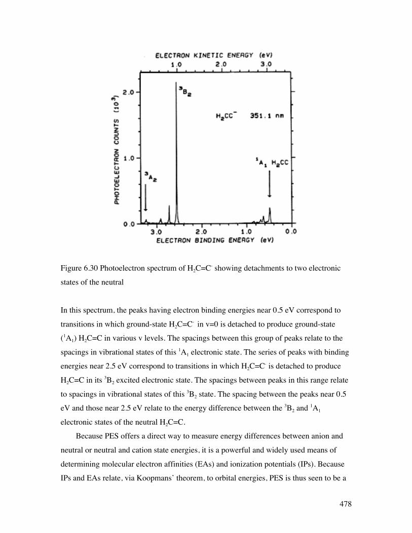
478

Figure 6.30 Photoelectron spectrum of H2C=C- showing detachments to two electronic

states of the neutral

In this spectrum, the peaks having electron binding energies near 0.5 eV correspond to

transitions in which ground-state H2C=C- in v=0 is detached to produce ground-state

(1A1) H2C=C in various v levels. The spacings between this group of peaks relate to the

spacings in vibrational states of this 1A1 electronic state. The series of peaks with binding

energies near 2.5 eV correspond to transitions in which H2C=C- is detached to produce

H2C=C in its 3B2 excited electronic state. The spacings between peaks in this range relate

to spacings in vibrational states of this 3B2 state. The spacing between the peaks near 0.5

eV and those near 2.5 eV relate to the energy difference between the 3B2 and 1A1

electronic states of the neutral H2C=C.

Because PES offers a direct way to measure energy differences between anion and

neutral or neutral and cation state energies, it is a powerful and widely used means of

determining molecular electron affinities (EAs) and ionization potentials (IPs). Because

IPs and EAs relate, via Koopmans’ theorem, to orbital energies, PES is thus seen to be a

479

way to measure orbital energies. Its vibrational envelopes also offer a good way to probe

vibrational energy level spacings, and hence the bonding strengths.

6.2.3 Probing Continuum Orbitals

There is another type of spectroscopy that can be used to directly probe the orbitals

of a molecule that lie in the continuum (i.e., at energies higher than that of the parent

neutral). I ask that you reflect back on our discussion in Chapter 2 of tunneling and of

resonance states that can occur when an electron experiences both attractive and repulsive

potentials. In such cases, there exists a special energy at which the electron can be

trapped by the attractive potential and have to tunnel through the repulsive barrier to

eventually escape. It is these kinds of situations that this spectroscopy probes.

This experiment is called electron-transmission spectroscopy (ETS). In such an

experiment, a beam of electrons having a known intensity I0 and narrowly defined range

of kinetic energies E is allowed to pass through a sample (usually gaseous) of thickness

L. The intensity I of electrons observed to pass through the sample and arrive at a

detector lying along the incident beam’s direction is monitored, as are the kinetic energies

of these electrons E’. Such an experiment is described in qualitative form in Fig. 6.31.

Figure 6.31 Qualitative depiction of a prototypical electron transmission spectrum setup.

Intensity ofIncident ElectronBeam I0

Intensity ofTransmittedElectron Beam I

Sample of thickness L

480

If the molecules in the sample have a resonance orbital whose energy is close to the

kinetic energy E of the colliding electrons, it is possible for an electron from the beam to

be captured into such an orbital and to exist in this orbital for a considerable time. Of

course, in the absence of any collisions or other processes to carry away excess energy,

this anion will re-emit an electron at a later time. Hence, such anions are called

metastable and their electronic states are called resonance states. If the captured electron

remains in this orbital for a length of time comparable to or longer than the time it takes

for the nascent molecular anion to undergo vibrational or rotational motion, various

events can take place before the electron is re-emitted:

i. some bond lengths or angles can change (this will happen if the orbital occupied by

the beam’s electron has bonding or antibonding character) so, when the electron is

subsequently emitted, the neutral molecule is left with a change in vibrational

energy;

ii. the molecule may rotate, so when the electron is ejected, it is not emitted in the same

direction as the incident beam.

In the former case, one observes electrons emitted with energies E’ that differ from that

of the incident beam by amounts related to the internal vibrational energy levels of the

anion. In the latter, one sees a reduction in the intensity of the beam that is transmitted

directly through the sample and electrons that are scattered away from this direction.

Such an ETS spectrum is shown in Fig. 6.32 for a gaseous sample of CO2 molecules.

In this spectrum, the energy of the transmitted beam’s electrons is plotted on the

horizontal axis and the derivative of the intensity of the transmitted beam is plotted on the

vertical axis. It is common to plot such derivatives in ETS-type experiments to allow the

variation of the signal with energy to be more clearly identified.

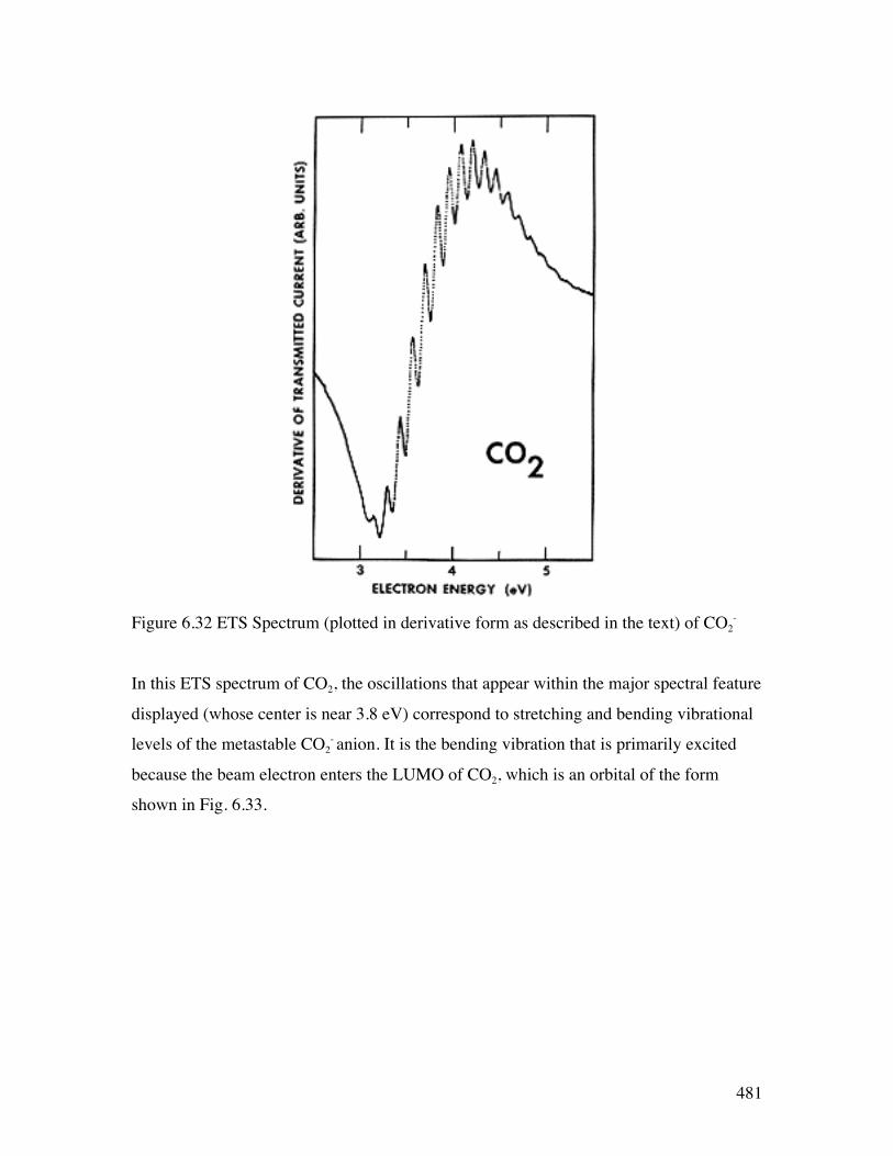
481

Figure 6.32 ETS Spectrum (plotted in derivative form as described in the text) of CO2

-

In this ETS spectrum of CO2, the oscillations that appear within the major spectral feature

displayed (whose center is near 3.8 eV) correspond to stretching and bending vibrational

levels of the metastable CO2- anion. It is the bending vibration that is primarily excited

because the beam electron enters the LUMO of CO2, which is an orbital of the form

shown in Fig. 6.33.

482

Figure 6.33 Antibonding π* orbital of CO2 holding the excess electron in CO2-

Occupancy of this antibonding π* orbital, causes both C-O bonds to lengthen and the

O-C-O angle to bend away from 180 deg. The bending allows the antibonding nature of

this orbital to be reduced.

Other examples of ETS spectra are shown in Fig. 6.34.

O C O

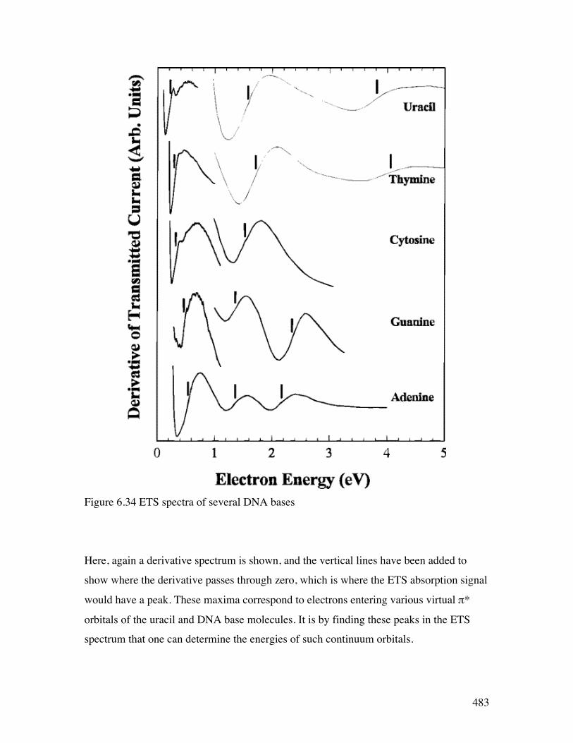
483

Figure 6.34 ETS spectra of several DNA bases

Here, again a derivative spectrum is shown, and the vertical lines have been added to

show where the derivative passes through zero, which is where the ETS absorption signal

would have a peak. These maxima correspond to electrons entering various virtual π*

orbitals of the uracil and DNA base molecules. It is by finding these peaks in the ETS

spectrum that one can determine the energies of such continuum orbitals.

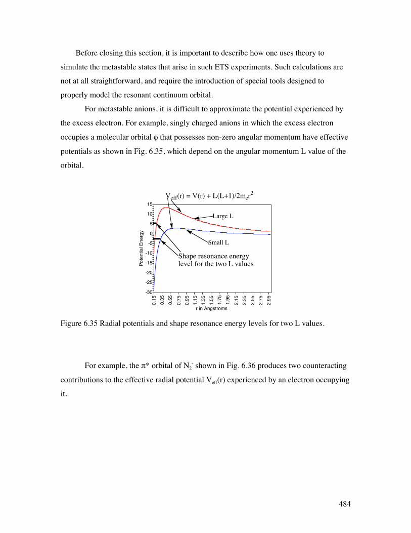
484

Before closing this section, it is important to describe how one uses theory to

simulate the metastable states that arise in such ETS experiments. Such calculations are

not at all straightforward, and require the introduction of special tools designed to

properly model the resonant continuum orbital.

For metastable anions, it is difficult to approximate the potential experienced by

the excess electron. For example, singly charged anions in which the excess electron

occupies a molecular orbital φ that possesses non-zero angular momentum have effective

potentials as shown in Fig. 6.35, which depend on the angular momentum L value of the

orbital.

0.15

0.35

0.55

0.75

0.95

1.15

1.35

1.55

1.75

1.95

2.15

2.35

2.55

2.75

2.95

-30

-25

-20

-15

-10

-5

0

5

10

15

Pote

ntia

l Ene

rgy

r in Angstroms

Veff(r) = V(r) + L(L+1)/2mer2

Large L

Small L

Shape resonance energylevel for the two L values

Figure 6.35 Radial potentials and shape resonance energy levels for two L values.

For example, the π* orbital of N2- shown in Fig. 6.36 produces two counteracting

contributions to the effective radial potential Veff(r) experienced by an electron occupying

it.

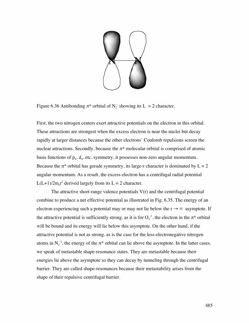
485

NN

Figure 6.36 Antibonding π* orbital of N2- showing its L = 2 character.

First, the two nitrogen centers exert attractive potentials on the electron in this orbital.

These attractions are strongest when the excess electron is near the nuclei but decay

rapidly at larger distances because the other electrons’ Coulomb repulsions screen the

nuclear attractions. Secondly, because the π* molecular orbital is comprised of atomic

basis functions of pπ, dπ, etc. symmetry, it possesses non-zero angular momentum.

Because the π* orbital has gerade symmetry, its large-r character is dominated by L = 2

angular momentum. As a result, the excess electron has a centrifugal radial potential

L(L+1)/2mer2 derived largely from its L = 2 character.

The attractive short-range valence potentials V(r) and the centrifugal potential

combine to produce a net effective potential as illustrated in Fig. 6.35. The energy of an

electron experiencing such a potential may or may not lie below the r → ∞ asymptote. If

the attractive potential is sufficiently strong, as it is for O2-1, the electron in the π* orbital

will be bound and its energy will lie below this asymptote. On the other hand, if the

attractive potential is not as strong, as is the case for the less-electronegative nitrogen

atoms in N2-1, the energy of the π* orbital can lie above the asymptote. In the latter cases,

we speak of metastable shape-resonance states. They are metastable because their

energies lie above the asymptote so they can decay by tunneling through the centrifugal

barrier. They are called shape-resonances because their metastability arises from the

shape of their repulsive centrifugal barrier.

486

If one had in-hand a reasonable approximation to the attractive short-range

potential V(r) and if one knew the L-symmetry of the orbital occupied by the excess

electron, one could form Veff(r) as above. However, to compute the lifetime of the shape

resonance, one has to know the energy E of this state. The most common and powerful

tool for studying such metastable states theoretically is the stabilization method (SM) that

Prof. Howard Taylor at USC (http://chem.usc.edu/faculty/Taylor.html) pioneered. This

method involves embedding the system of interest (e.g., the N2-1 anion) within a finite

radial box in order to convert the continuum of states corresponding, for example, to N2 +

e-, into discrete states that can be handled using more conventional methods. By then

varying the size of the box, one can vary the energies of the discrete states that

correspond to N2 + e- (i.e., one varies the kinetic energy KE of the orbital containing the

excess electron). As the box size is varied, one eventually notices (e.g., by plotting the

orbitals) that one of the N2 + e- states possesses a significant amount of valence (i.e.,

short-range) character. That is, one such state has significant amplitude not only at large-r

but also in the region of the two nitrogen centers. It is this state that corresponds to the

metastable shape-resonance state, and it is the energy E where significant valence

components develop that provides the stabilization estimate of the state energy.

Let us continue using N2-1 as an example for how the SM would be employed,

especially how one usually varies the box within which the anion is constrained. One

would use a conventional atomic orbital basis set that would likely include s and p

functions on each N atom, perhaps some polarization d functions and some conventional

diffuse s and p orbitals on each N atom. These basis orbitals serve primarily to describe

the motions of the electrons within the usual valence regions of space.

To this basis, one would append extra sets of diffuse π-symmetry orbitals. These

orbitals could be pπ (and maybe dπ) functions centered on each nitrogen atom, or they

could be pπ (and maybe dπ) orbitals centered at the midpoint of the N-N bond. One

usually would not add just one such function; rather several such functions, each with an

orbital exponent αJ that characterizes its radial extent, would be used. Let us assume, for

example, that K such π functions have been used.

Next, using the conventional atomic orbital basis as well as the K extra π basis

functions, one carries out a calculation (most often a variational calculation in which one

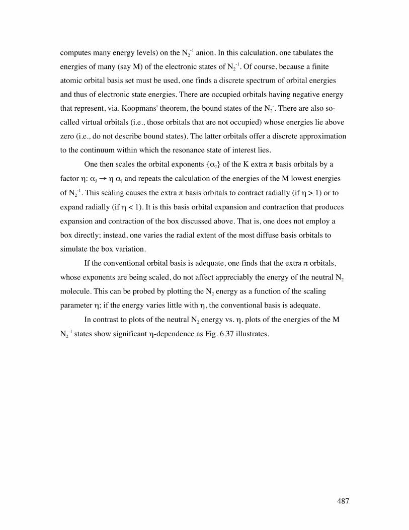
487

computes many energy levels) on the N2-1 anion. In this calculation, one tabulates the

energies of many (say M) of the electronic states of N2-1. Of course, because a finite

atomic orbital basis set must be used, one finds a discrete spectrum of orbital energies

and thus of electronic state energies. There are occupied orbitals having negative energy

that represent, via. Koopmans' theorem, the bound states of the N2-. There are also so-

called virtual orbitals (i.e., those orbitals that are not occupied) whose energies lie above

zero (i.e., do not describe bound states). The latter orbitals offer a discrete approximation

to the continuum within which the resonance state of interest lies.

One then scales the orbital exponents {αJ} of the K extra π basis orbitals by a

factor η: αJ → η αJ and repeats the calculation of the energies of the M lowest energies

of N2-1. This scaling causes the extra π basis orbitals to contract radially (if η > 1) or to

expand radially (if η < 1). It is this basis orbital expansion and contraction that produces

expansion and contraction of the box discussed above. That is, one does not employ a

box directly; instead, one varies the radial extent of the most diffuse basis orbitals to

simulate the box variation.

If the conventional orbital basis is adequate, one finds that the extra π orbitals,

whose exponents are being scaled, do not affect appreciably the energy of the neutral N2

molecule. This can be probed by plotting the N2 energy as a function of the scaling

parameter η; if the energy varies little with η, the conventional basis is adequate.

In contrast to plots of the neutral N2 energy vs. η, plots of the energies of the M

N2-1 states show significant η-dependence as Fig. 6.37 illustrates.

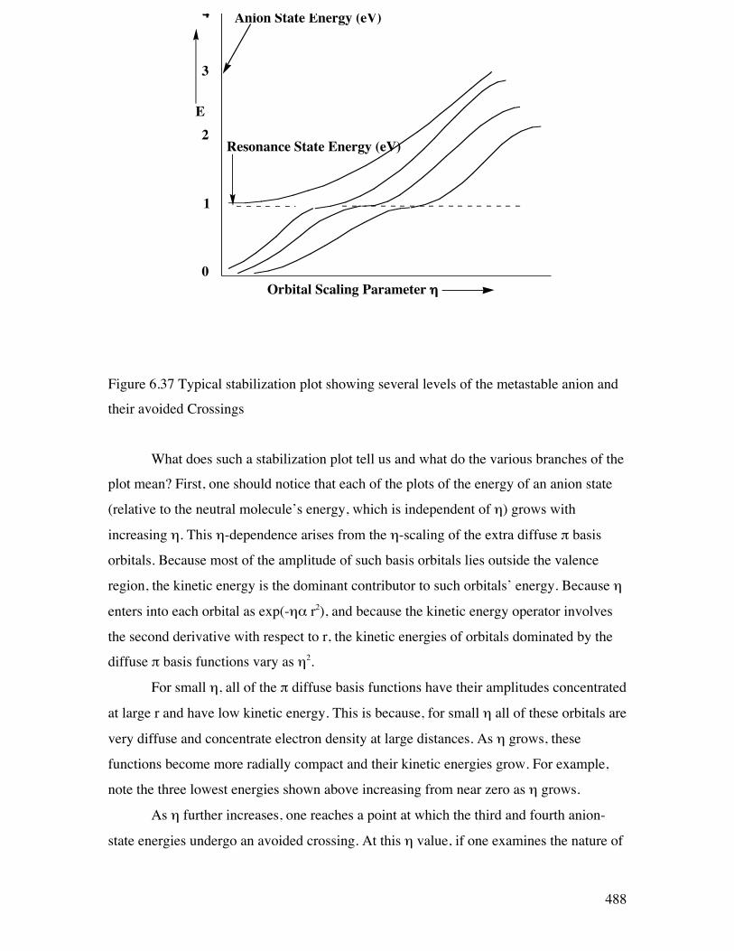
488

Figure 6.37 Typical stabilization plot showing several levels of the metastable anion and

their avoided Crossings

What does such a stabilization plot tell us and what do the various branches of the

plot mean? First, one should notice that each of the plots of the energy of an anion state

(relative to the neutral molecule’s energy, which is independent of η) grows with

increasing η. This η-dependence arises from the η-scaling of the extra diffuse π basis

orbitals. Because most of the amplitude of such basis orbitals lies outside the valence

region, the kinetic energy is the dominant contributor to such orbitals’ energy. Because η

enters into each orbital as exp(-ηα r2), and because the kinetic energy operator involves

the second derivative with respect to r, the kinetic energies of orbitals dominated by the

diffuse π basis functions vary as η2.

For small η, all of the π diffuse basis functions have their amplitudes concentrated

at large r and have low kinetic energy. This is because, for small η all of these orbitals are

very diffuse and concentrate electron density at large distances. As η grows, these

functions become more radially compact and their kinetic energies grow. For example,

note the three lowest energies shown above increasing from near zero as η grows.

As η further increases, one reaches a point at which the third and fourth anion-

state energies undergo an avoided crossing. At this η value, if one examines the nature of

Orbital Scaling Parameter η

Anion State Energy (eV)

Resonance State Energy (eV)

E

0

1

2

3

4

489

the two wave functions whose energies avoid one another, one finds that one of them

contains substantial amounts of both valence and extra-diffuse π function character. Just

to the left of the avoided crossing, the lower-energy state (the third state for small η)

contains predominantly extra diffuse π orbital character, while the higher-energy state

(the fourth state) contains largely valence π* orbital character.

However, at the special value of η where these two states nearly cross, the kinetic

energy of the third state (as well as its radial size and its de Broglie wavelength) are

appropriate to connect properly with the fourth state. By connect properly we mean that

the two states have wave function amplitudes, phases, and slopes that match. So, at this

special η value, one can achieve a description of the shape-resonance state that correctly

describes this state both in the valence region and in the large-r region. Only by tuning

the energy of the large-r states using the η scaling can one obtain this proper boundary

condition matching.

In summary, by carrying out a series of anion-state energy calculations for several

states and plotting them vs. η, one obtains a stabilization graph. By examining this graph

and looking for avoided crossings, one can identify the energies at which metastable

resonances occur. It is also possible to use the shapes (i.e., the magnitude of the energy

splitting between the two states and the slopes of the two avoiding curves) of the avoided

crossings in a stabilization graph to compute the lifetimes of the metastable states.

Basically, the larger the avoided crossing energy splitting between the two states, the

shorter is the lifetime of the resonance state.

So, the ETS and PES experiments offer wonderful probes of the bound and

continuum states of molecules and ions that tell us a lot about the electronic nature and

chemical bonding of these species. The theoretical study of these phenomena is

complicated by the need to properly identify and describe any continuum orbitals and

states that are involved. The stabilization technique allows us to achieve a good

approximation to resonance states that lie in such continua.

6.3 Chapter Summary

In this Chapter, you were introduced to many of the main topics of electronic

structure theory. The subjects you should now be familiar with include

490

a. The Hatree and Hartree-Fock models,

b. Koopmans’theorem

c. Atomic basis functions- Slater and Gaussian- and the notations used to describe them.

d. Static and dynamic electron correlation.

e. The CI, MPPT, CC, and DFT methods for treating correlation, as well as EOM or

Greens function methods.

f. The Slater-Condon rules.

g. QM-MM methods.

h. Experimental tools to probe electronic structures including methods for metastable

states.

i. Various contributions to spectroscopic line shapes and line broadening.