169

CHAPTER 6

HYBRID EVOLUTIONARY ALGORITHMS

6.1 INTRODUCTION

In recent years, the performance of computers has a great influence

over the power systems in maintaining quality and reliable power supply.

Furthermore, the power system can be controlled easily and efficiently with a

higher degree of reliability. The growth in size and complexity of electric

power systems along with an increase in power demand has initiated the need

for intelligent systems that combine different techniques and methodologies.

The intelligent systems possess human like expert knowledge and adapt

themselves in changing environments. In the electric power system, as the

demand deviates from its normal value with an unpredictable small amount,

the state of the system changes. The automatic control system detects these

changes and initiates real time control actions, which will eliminate as

effectively and quickly as possible the state deviations. The active and

reactive power demands are never steady but continuously change with rising

and falling trend (Hadi Saadat 2002). Steam input to turbo- generators must

therefore be continually regulated to match the active power demand, failing

which the machine speed will vary with consequent change in frequency,

which may be highly undesirable. Furthermore, the excitation of generators

must be continually regulated to match the reactive power demand with

reactive generation, otherwise the voltages at various system buses may go

beyond the prescribed limits (Kundur2006).

170

Automatic Generation Control (AGC) is used in real-time control

to match the area generation changes to area load changes in order to meet tie-

line flows and keep the frequency at nominal value. By processing frequency

and tie-line deviations, AGC can determine the load changes of its own area

and in its neighbouring area. The function of AGC is to reallocate the

generation changes to pre-selected machines after an initial random

accommodation of the load by governor action. It is necessary to obtain much

better frequency constancy than obtained by the speed governor itself (Wood

and Wollenberg 2003). For successful operation of the power system, the load

must be fed with constant voltage and frequency. Hence, a suitable control

strategy has to be developed to accomplish this task. In practice different

control strategies are utilized for AGC like, Proportional and Integral (PI),

Proportional, Integral and Derivative (PID) and optimal control (Vinodkumar

1998). The optimal control is often impractical for the implementation, since

accurate prediction of load demand is necessary (Murthy 2009).

The PID controller is by far the most commonly used controller in

process control applications. It performs important functions like, the

elimination of steady-state off -set and anticipation of deviation and

generation of adequate corrective signals through the derivative action.

Together with combinational logic, sequential machines and simple function

blocks, these PID controllers are increasingly being used to build the

automation system for industries. Even though these PID controllers are very

common and well known, they are often not tuned properly resulting in poor

control quality. Since almost all PID controllers are implemented in software,

there is an opportunity to incorporate complex algorithms in these controllers.

Auto-tuning is one such feature, which is being extensively used in

commercially available PID controllers (Bandyopadhyay et al 2001). The

performances of the control loops are improved by auto tuning the PID gain

parameters of conventional controllers.

171

In many engineering disciplines a large spectrum of optimization

problems has grown in size and complexity. In some instances, the solution to

complex multidimensional problems by using classical optimization

techniques is sometimes difficult and/or computationally expensive. Hence,

Evolutionary Algorithms (EA) have been applied successfully to many

complex problems in the field of industrial and operational engineering. In

power systems, EA is applied to well-known applications including,

generation planning, network planning, unit commitment, economic dispatch,

load forecasting, power quality and reliability studies. However, as a

consequence of the structural changes in the electric power industry and need

for more advanced controllers, the incorporation of hybrid optimization

methods in the decision-making process has become ineviTable Moreover,

the industry restructuring introduces a wide range of new optimization tasks

characterized by their complexity and the amount of variables involved in the

optimization process. In some instances, the solution of these multidimensional

problems by classical optimization techniques is difficult or even impossible.

Hence, to deal with these types of optimization problems, a special class of

hybrid algorithms have received increased attention regarding their potential

in solving complex problems. In this research, hybridization is achieved by

combining basic PSO algorithm with fuzzy, GA and BF for optimal tuning of

PID gains. This improves the local and global search ability of PSO and

overcomes the premature convergence problem associated with large scale

and complex applications.

Shi and Eberhart (2001) proposed a hybrid system for three test

functions by using fuzzy to adjust dynamicallythe inertia weight to improve

the performance of the PSO. Simulation results illustrate the performance

improvement of PSO when tested for three benchmark functions. Buczak and

Uhrig (1996) proposed a novel hierarchical fuzzy-genetic information fusion

technique. The combined reasoning takes place by fuzzy aggregation

172

functions, capable of combining information by compensatory connectives

that better mimic the human reasoning process than union and intersection,

employed in traditional set theories. The simulation results validate the

performance of the fusion algorithm with reduced computational complexity

and generate satisfactory results. Wenping Chang (2010) presented a novel

fuzzy adaptive PSO to determine the optimal operation of the hydrothermal

power system. The experimental result shows that the proposed approach has

the higher quality solutions and strong ability in global search. Gomez

Skarmeta et al (2001) evaluated the use of combining the fuzzy clustering

techniques with GA for classification tasks and the potential of their

integration in producing better classification results. The results show that the

use of the hybrid algorithm could increase the accuracy of the system in

comparison with the conventional GA technique. Li Zang et al (2010)

proposed PSO-fuzzy group decision making support system for vehicle

performance evaluation. The performance analysis reveals that the PSO-fuzzy

is an efficient method, and it can be used to solve complex problems in the

field of power system engineering. Mahdi Banejad and Hooshmand (2001)

have presented Fuzzy PSO algorithm for optimal design of PID controller in

an AVR system and the performance was found to be better when compared

with conventional GA and PSO algorithms. Bandyopadhyay et al (2001) have

presented Fuzzy-GA approach for auto-tuning of PID controller for different

process models. The responses of first-order dead-time process model and

second-order dead-time process models were presented, and satisfactory

responses were achieved. Fang and Chen (2009) proposed an enhanced PSO

(EPSO) algorithm for optimal tuning of PID gains for a typical PID control

system. The simulation results show that the EPSO algorithm has stable

convergence characteristics and good computational stability.

Dong Hwa Kim et al (2007) proposed hybrid GA-BF approach for

global optimization problems and its performance was validated for four test

173

functions and to tune the gains of PID controller in AVR system. Simulation

results of test functions and AVR clearly indicated the efficiency of proposed

approach, and therefore, it could be used to solve different optimization

problems. ArijitBiswas et al (2007) proposed a hybrid approach involving

PSO and BF algorithm for optimizing multimodal and high dimensional

functions. The new method found to be statistically better, since the proposed

algorithm outperformed both GA and BF over few numerical benchmarks and

in optimizing PID gain parameters. Wong et al (2009) developed hybrid

evolutionary algorithm combining GA and PSO for PID controller design for

AVR system. From comparison and simulation results, it is found that the

proposed new algorithm finds a high quality solution effectively. ArijitBiswas

(2007) designed a hybrid optimization technique, which synergistically

couples the BF with the PSO. The proposed algorithm has shown to be

statistically better and can be used significantly in designing optimization

problem. Mukherjee and Ghosal (2008), Shayeghi (2007, 2008), Ghosal and

Goswami (2003), Ghosal (2004) have developed EA Based algorithms to

optimize the PID gains for adaptive control applications and thereby

increasing the performance characteristics of a controller. Sabahi et al (2008)

proposed adaptive weighted particle swarm optimization for LFC in two areas

interconnected power system. The simulation results validate the efficiency of

improved PSO algorithm in obtaining the frequency response characteristics.

From the simulation results, the efficiency of proposed controller design is

obtained and compared with the conventional PSO with. Seyed Abbas Taher

et al (2008) developed hybrid PSO (HPSO) algorithm for optimal

decentralized LFC in two area power system. Simulation results indicate that

HPSO controller guarantee the good performance under various load

conditions.

In this research, an advanced hybrid EA is proposed to increase the

searching speed, reliability and efficiency of the original PSO algorithm. The

174

proposed hybrid intelligent paradigms exhibit an ability to adapt and learn to

new applications or situations under changing environment. This technique

puts the adaptively changing terms in original constant terms, so that the

parameters of the original PSO algorithm changes with convergence rate,

which is presented by the objective function. In order to identify the changing

dynamics of the power system and to provide appropriate control actions, fast

dynamic models are needed. The model of the LFC and AVR of a single area

power system is designed using simulink in MATLAB. The objective of this

work is to design and implement hybrid EA Based PID controller to search

the optimal PID gain parameters for efficient control of voltage and

frequency. The evolutionary algorithms proposed in this research are

Enhanced Particle Swarm Optimization (EPSO), Multi objective Particle

Swarm Optimization (MOPSO) and Stochastic Particle Swarm Optimization

(SPSO), Fuzzy Particle Swarm Optimization (FPSO), Bacterial Foraging

Particle Swarm Optimization (BF-PSO) and Hybrid Genetic Algorithm

(HGA). The algorithms are designed to generate the optimum Proportional,

Integral and Derivative gains of the controller. These values are sent to

workspace and shared with the simulink model for simulation under various

loads and regulation parameters. The proposed LFC and AVR contribute to

the satisfactory operation of the power system by maintaining system voltages

and frequency for different load and regulation parameters.

This chapter is organized as follows: Section 2 describes the types

of hybrid EA; Section 3 describes the design of hybrid EA Based controllers;

Section 4 shows simulation results. Performance comparison of different

hybrid EA is given in section 5. Section 6 indicates the computational

efficiency of hybrid controllers, and summary is derived in Section 7.

175

6.2 EVOLUTIONARY ALGORITHMS

Evolutionary Algorithm (EA) is a basic search algorithm, which is

derived from the Darwin’s Theory of Evolution, proposed in 1859. According

to the Darwin’s theory, if an environment can host only a limited number of

populations then every single individual in the environment tries to attain the

best position. As a result, the individuals will begin to compete among

themselves for the given resources to attain a better position and at last, the

individuals that are best fit to the environmental conditions will survive. This

phenomenon is also known as ‘survival of the fittest’. The mechanisms used

by EAs are inspired from biological evolution to find the solution for the

given problem. It performs well in approximating a set of solution for all

types of problems because they ideally do not make any assumption about the

underlying fitness landscape. The Evolutionary process is simulated in a

computer and hence, millions of generations can be executed in a matter of

hours and can be repeated under various circumstances. Evolution is an

optimization process, where the aim is to improve the ability of individuals to

survive. Evolution via natural selection of a randomly chosen population of

individuals can be thought of as a search through the space of possible

chromosome values. In that sense, an EA is a stochastic search for an optimal

solution to a given problem. An EA utilizes a population of individuals,

where everyone represents a candidate solution to the problem.

The EA selects the best fit value from the given population, and it

is less sensitive to the scaling of algorithm parameters. EA also has good fault

tolerance, and it furthermore takes care of social and cognition behavior of the

individual particle. In Evolutionary algorithm, the self-adaption of the particle

is an important strategy which varies the EA parameters during run time in a

specific manner. This feature is inherent in modern evolution strategies and

176

provided the context of changing fitness landscapes also. With this feature,

even if the objective function changes, the EA always aims at the moving

target i.e. the present population will be reevaluated, and quite naturally it is

tested whether individuals have been adapted to the new objective function.

The EA techniques provide robust performance and global search

characteristics. The most significant advantage of using EA technique is the

gain of flexibility and adaptability to the task for which the algorithm is

designed (Fogel 2000). Hybrid EA spans a family of optimization algorithms,

each algorithm is differentiated by the way of selecting the best solution,

method of creating new solutions from existing ones, and the data structures

used to represent those solutions. The different variants of the PSO algorithm

described in this section incorporate either the capabilities of other

computation techniques like Fuzzy, GA, BF or the adaptation of PSO

parameters for a better performance. The proposed hybridization techniques

presented in this section has superior features, including easy implementation,

stable convergence characteristics and good computational efficiency.

6.2.1 Enhanced Particle Swarm Optimization (EPSO)

The EPSO is an improved version of the conventional PSO, being

inspired by the study of birds and fish flocking. In EPSO, the Constriction

Factor approach is introduced in the velocity update formula to ensure faster

convergence. In EPSO algorithm, each particle in the swarm represents a

solution to the problem and it is defined with its position and velocity. In

D-dimensional search space, the position of the ith

particle can be represented

by a D-dimensional vector, Xi= (Xi1,…,Xid, …, XiD). The velocity of the

particle vi can be represented by another D-dimensional vector Vi= (Vi1,…,

Vid, …, ViD). The best position visited by the ith

particle is denoted as

Pi= (Pi1,…,Pid,…,PiD), and Pg as the index of the particle visited the best

177

position in the swarm, then Pg becomes the best solution found so far. The

working of EPSO algorithm is explained in the following steps.

Step 1: The algorithm parameters like number of generation, population

size, inertia weight minimum, maximum (Wmin, Wmax), and maximum

iterations are initialized.

Step 2: The values of Kp, Ki and Kd are initialized randomly within the

optimal range of values for each gains.

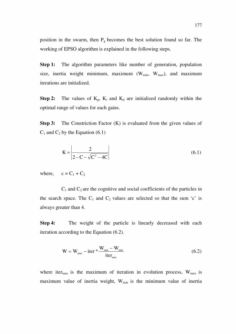
Step 3: The Constriction Factor (K) is evaluated from the given values of

C1 and C2 by the Equation (6.1)

C4CC2

2K

2 (6.1)

where, c = C1 + C2

C1 and C2 are the cognitive and social coefficients of the particles in

the search space. The C1 and C2 values are selected so that the sum ‘c’ is

always greater than 4.

Step 4: The weight of the particle is linearly decreased with each

iteration according to the Equation (6.2).

max

minmin

maxiter

WW*iterWW (6.2)

where itermax is the maximum of iteration in evolution process, Wmax is

maximum value of inertia weight, Wmin is the minimum value of inertia

178

weight, and iter is current value of iteration and the weight ‘W’ is updated in

every iteration.

Step 5: The fitness of each particle is evaluated using the Integral of Time

multiplied by the Absolute value of Error (ITAE) fitness function as in

Equation (6.3)

0dt).t(e.tF (6.3)

Step 6: The Local Best position (Pi) and the Global Best position (Pg) of

particles are found Based on the fitness value of the particles calculated from

step 5.

Step 7: The velocity and position of the particle is updated using the

Equation (6.4) and Equation (6.5) respectively.

Vid = WKVid + C1 R (Pid – Xid) + C2r (Pgd– Xid) (6.4)

Xid=Xid+Vid (6.5)

where R and r are random numbers selected between 0 and 1.

Step 8: The steps 4 to 7 are repeated until the maximum iterations reached or

the best solution is found.

The variables used in EPSO algorithm and their definitions are

tabulated in Table 6.1.

179

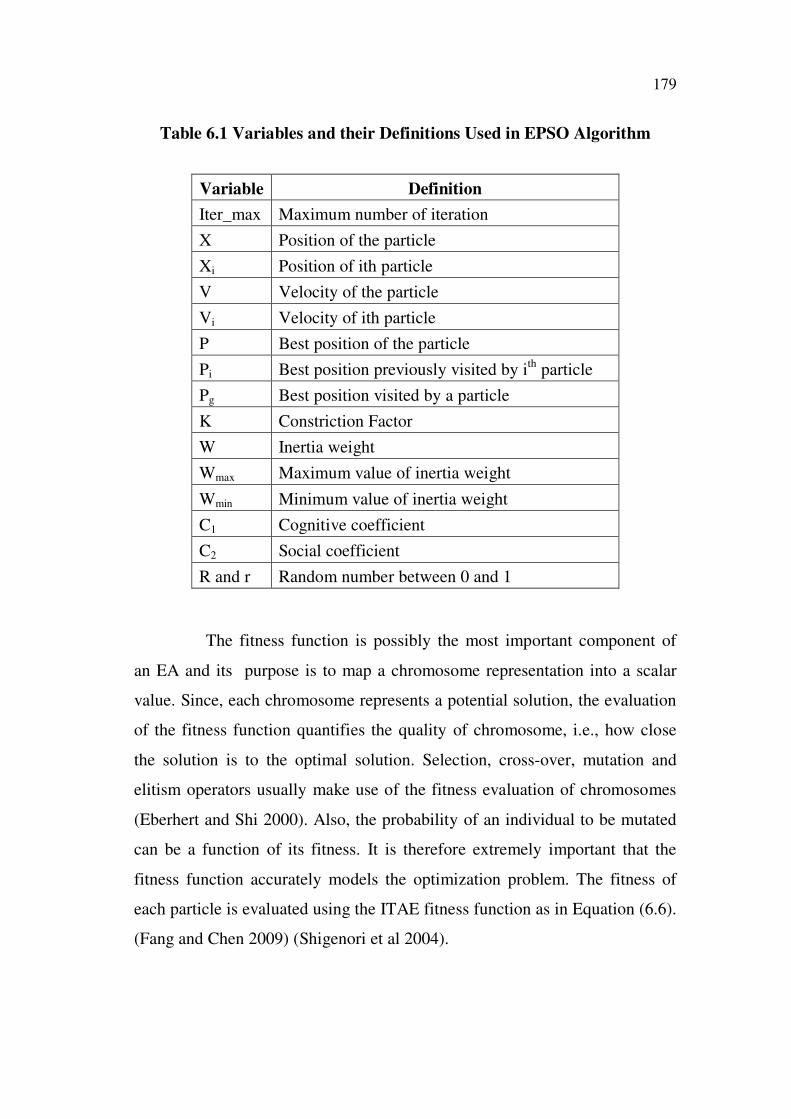
Table 6.1 Variables and their Definitions Used in EPSO Algorithm

Variable Definition

Iter_max Maximum number of iteration

X Position of the particle

Xi Position of ith particle

V Velocity of the particle

Vi Velocity of ith particle

P Best position of the particle

Pi Best position previously visited by ith

particle

Pg Best position visited by a particle

K Constriction Factor

W Inertia weight

Wmax Maximum value of inertia weight

Wmin Minimum value of inertia weight

C1 Cognitive coefficient

C2 Social coefficient

R and r Random number between 0 and 1

The fitness function is possibly the most important component of

an EA and its purpose is to map a chromosome representation into a scalar

value. Since, each chromosome represents a potential solution, the evaluation

of the fitness function quantifies the quality of chromosome, i.e., how close

the solution is to the optimal solution. Selection, cross-over, mutation and

elitism operators usually make use of the fitness evaluation of chromosomes

(Eberhert and Shi 2000). Also, the probability of an individual to be mutated

can be a function of its fitness. It is therefore extremely important that the

fitness function accurately models the optimization problem. The fitness of

each particle is evaluated using the ITAE fitness function as in Equation (6.6).

(Fang and Chen 2009) (Shigenori et al 2004).

180

Start

Initialize the population and values of wmax,

wmin, C1, C2, itermax

Initialize Kp, Ki and Kd values randomly

Evaluate the Constriction Factor (K)

Update the weight of each particle

Calculate the Fitness function

Find the local and global best position of the particles

Calculate the fitness of the new population

Maximum

iterations

reached?

Output the parameters Kp, Ki and Kd

Stop

Yes

No

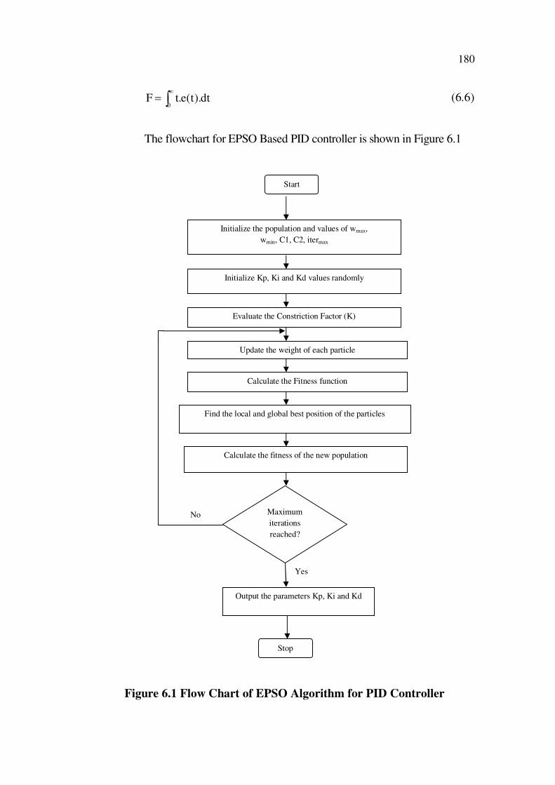
0dt).t(e.tF (6.6)

The flowchart for EPSO Based PID controller is shown in Figure 6.1

Figure 6.1 Flow Chart of EPSO Algorithm for PID Controller

181

The objective function provides a means for evaluating the

performance of the PID controller by determining the gain parameters in the

process of search, so that an optimized controller would be developed by the

best individual. The proposed EPSO algorithm provides stable and faster

convergence towards global best solution in a minimal computational time.

6.2.2 Multi Objective Particle Swarm Optimization (MOPSO)

Real world problems often have multiple conflicting objectives. In

certain problems, there is no single solution that is the best when measured on

all objectives. In this method, the acceleration Factor (K) is introduced in the

velocity update formula and the Inertia weight of the each particle is made to

decrease linearly in all iterations. By adjusting the different objectives, the

MOPSO seeks to discover possible combinations of available objectives and

then the best solutions can be found for the PID controller (Popov 2005). In

this algorithm original PSO which operates in continuous space is extended to

operate on discrete binary variables. The extended version of PSO has been

proven to be very effective for static and dynamic optimization problems. The

multi objective particle swarm optimization technique is Based on the idea of

combining several objective functions that are need to be satisfied by solution.

The variables used in MO-PSO algorithm and their definitions are tabulated

in Table 6.2.

182

Table 6.2 Variables and their Definitions Used in MO-PSO Algorithm

Variable Definition

iter_max Maximum number of iteration

X Position of the particle

Xi Position of ith particle

V Velocity of the particle

Vij,t+1 Velocity of i

th particle

P Best position of the particle

pij,t Best position previously visited by i

th particle

pij,,gt Best position visited by a particle

Acceleration Factor

W Inertia weight

C1 Cognitive coefficient

C2 Social coefficient

R1and R2 Random number between 0 and 1

The following steps explain the procedure of MO-PSO algorithm

Step 1: First population pt is initialised, which contains the initial particles,

their positions xti and their initial velocities vt .

Step 2: The values of Kp, Ki and Kd are initialized randomly within the

optimal range of values for each gains.

Step 3: The acceleration Factor ( ) is evaluated from the Equation (6.7).

= 0 + t / T (6.7)

183

where t denotes current generation, T denotes the total number of generation

and 0 selected within the range 0.5 and 1.

Step 4: After evaluating population pt, initial archive At is generated with

non-dominated solutions in pt The weight of the particle is Linearly

Decreased with each iteration according to the Equation (6.8).

W= w0 + r*(1-w0) (6.8)

where w0 is the initial weight and r is a random number varies between 0 and 1

Step 5: The local guide for each particle is found using the function

findlb(At+1,xti) from the set of non-dominated solutions stored in the archive

At for each particle in the search space.

Step 6: Determine the velocity and position of ith

particle Vij,t and x

ij,t to

direct the swarm towards optimum solution.

Step 7: The velocity and position of the particle is updated using the

following Equation (6.9) and Equation (6.10) respectiveley,

Vij,t+1 = wV

ij,t + * (c1R1( p

ij,t – x

ij,t) + c2R2 (p

ij,,gt – x

ij,t)) (6.9)

Xij,t+1= x

ij,t + V

ij,t+1 (6.10)

The Local and Global best positions are updated after each iteration

Based on the fitness values of particles.

Step 8: The fitness value is calculated considering the objective function

using the relation in Equation (6.11).

n

1iiival )k(fw)k(E (6.11)

184

Step 9: The steps 2 to 8 are repeated until the maximum iteration reached or

the best solution is attained.

Each particle has to change its position xti towards the position of a

local guide pti.g

and its best personal position stored in pt. The particles in the

population pt will be evaluated by function chosen for the particular

application in this case, the objective function. An ideal fitness function

correlates closely with the algorithm's goal, and yet may be computed

quickly. Speed of execution is very important, as a typical evolutionary

algorithm must be iterated many times in order to produce a usable result for a

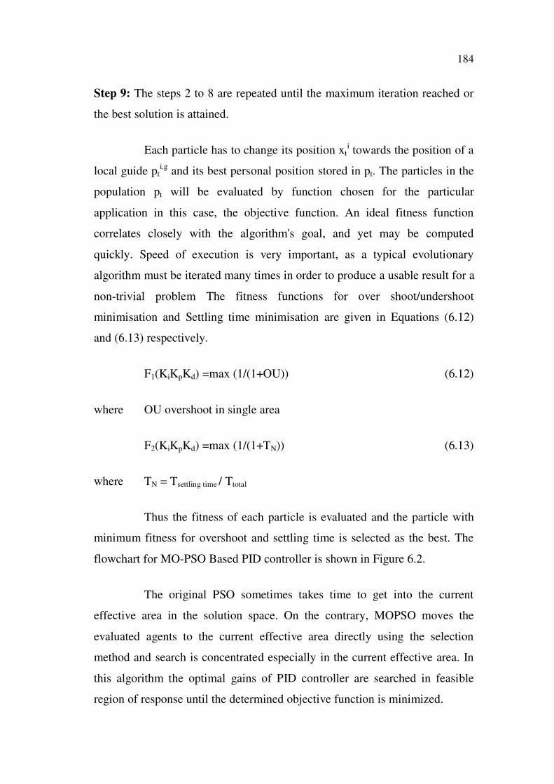
non-trivial problem The fitness functions for over shoot/undershoot

minimisation and Settling time minimisation are given in Equations (6.12)

and (6.13) respectively.

F1(KiKpKd) =max (1/(1+OU)) (6.12)

where OU overshoot in single area

F2(KiKpKd) =max (1/(1+TN)) (6.13)

where TN = Tsettling time / Ttotal

Thus the fitness of each particle is evaluated and the particle with

minimum fitness for overshoot and settling time is selected as the best. The

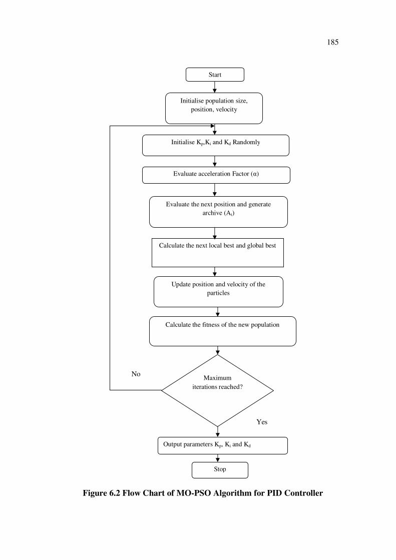
flowchart for MO-PSO Based PID controller is shown in Figure 6.2.

The original PSO sometimes takes time to get into the current

effective area in the solution space. On the contrary, MOPSO moves the

evaluated agents to the current effective area directly using the selection

method and search is concentrated especially in the current effective area. In

this algorithm the optimal gains of PID controller are searched in feasible

region of response until the determined objective function is minimized.

185

Initialise population size,

position, velocity

Calculate the next local best and global best

Update position and velocity of the

particles

Evaluate acceleration Factor ( )

Evaluate the next position and generate

archive (At)

Start

Initialise Kp,Ki and Kd Randomly

Calculate the fitness of the new population

Maximum

iterations reached?

Output parameters Kp, Ki and Kd

Stop

No

Yes

Figure 6.2 Flow Chart of MO-PSO Algorithm for PID Controller

186

6.2.3 Stochastic Particle Swarm Optimization (SPSO)

In this method, the ‘Time Varying Acceleration Co-efficient’s

(TVACs) are introduced for Cognitive and Social co-efficient. The

implementation of these TVAC’s reduces the cognitive component (C1)

meanwhile increasing the social component (C2) acceleration coefficient with

time. Here, the inertia weight and acceleration coefficients are neither set to a

constant value nor set as a linearly decreasing time varying function. Instead,

these values are updated non-linearly in each generation and so better

convergence rate is obtained towards the optimal PID gains in minimal

iterations (Janga Reddy and Nagesh Kumar 2007). The Time Varying

Acceleration Co-efficient (TVAC) i.e. Cognitive and Social Co-efficients are

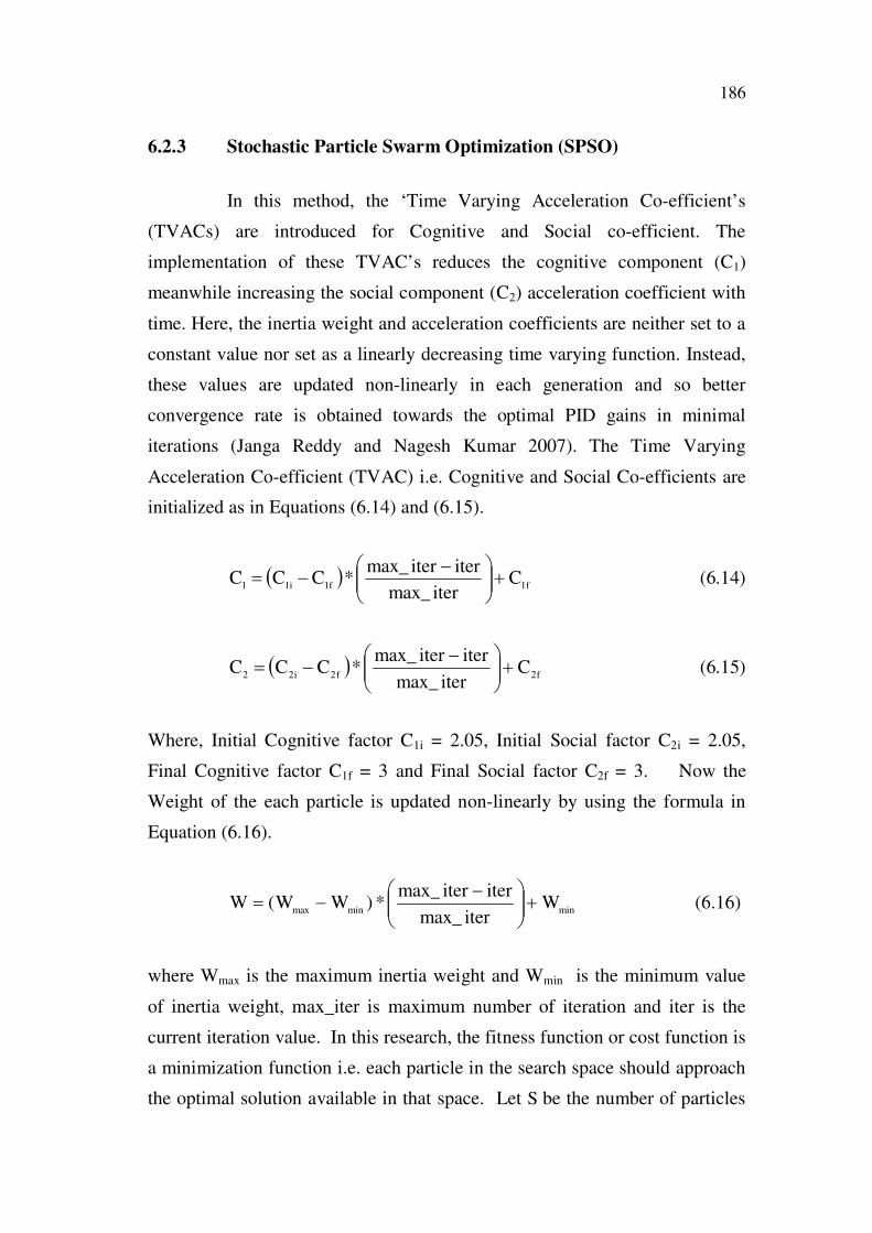
initialized as in Equations (6.14) and (6.15).

f1f1i11C

itermax_

iteritermax_*CCC (6.14)

f2f2i22C

itermax_

iteritermax_*CCC (6.15)

Where, Initial Cognitive factor C1i = 2.05, Initial Social factor C2i = 2.05,

Final Cognitive factor C1f = 3 and Final Social factor C2f = 3. Now the

Weight of the each particle is updated non-linearly by using the formula in

Equation (6.16).

minminmaxW

itermax_

iteritermax_*)WW(W (6.16)

where Wmax is the maximum inertia weight and Wmin is the minimum value

of inertia weight, max_iter is maximum number of iteration and iter is the

current iteration value. In this research, the fitness function or cost function is

a minimization function i.e. each particle in the search space should approach

the optimal solution available in that space. Let S be the number of particles

187

in the swarm, each particle will be in its own position i.e. xi Rn in the

N-dimensional search-space and its velocity Vi Rn. Let Pi be the current best

position of ith

particle and let ‘g’ be the Global best known position in the

entire swarm, the steps involved in SPSO algorithm are as follows

Step 1: The algorithm parameters like number of generations, number of

dimensions, Inertia weight minimum (Wmin), inertia weight maximum (Wmax),

initial and final values for Cognitive and social Co-efficient and maximum

iterations are initialized.

Step 2: The PID controller Gain values i.e. Kp,Ki,Kd are initialized randomly

within the optimal range.

Step 3: The Time Varying Acceleration Co-efficient (TVAC) i.e. Cognitive

(C1) and Social (C2) Co-efficients are initialized as in Equations (6.14) and

(6.15)

Step 4: The Weight of the each particle is updated non-linearly by using the

Equation (6.16)

Step 5: Fitness function is applied for each particle and it is evaluated in each

iteration for updating the particles towards the best solution in every step.

Step 6: Determine the local best position Pi and the Global best position Pg

among the particles, Based on the fitness function

Step 7: Now, the Velocity and Position of the Particle is updated by using the

Velocity and Position update formula i.e.,

Vid = w*Vid + c1R1( pid – xid) + c2R2 (pgd – xid) (6.17)

Xid = Xid+ Vid (6.18)

188

Thus, Local and Global best positions are updated for each iteration

using the fitness function and the solution move towards optimal value in

every step.

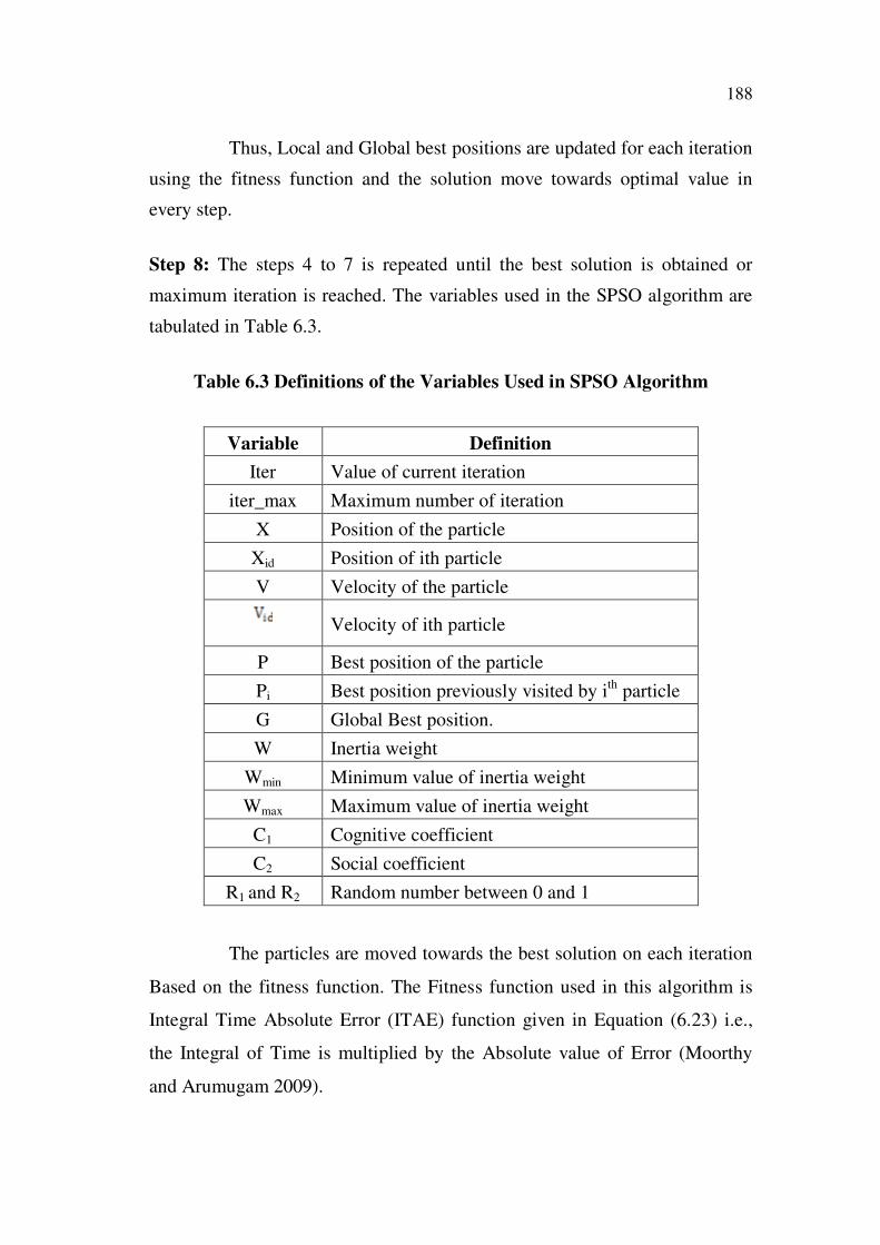
Step 8: The steps 4 to 7 is repeated until the best solution is obtained or

maximum iteration is reached. The variables used in the SPSO algorithm are

tabulated in Table 6.3.

Table 6.3 Definitions of the Variables Used in SPSO Algorithm

Variable Definition

Iter Value of current iteration

iter_max Maximum number of iteration

X Position of the particle

Xid Position of ith particle

V Velocity of the particle

Velocity of ith particle

P Best position of the particle

Pi Best position previously visited by ith

particle

G Global Best position.

W Inertia weight

Wmin Minimum value of inertia weight

Wmax Maximum value of inertia weight

C1 Cognitive coefficient

C2 Social coefficient

R1 and R2 Random number between 0 and 1

The particles are moved towards the best solution on each iteration

Based on the fitness function. The Fitness function used in this algorithm is

Integral Time Absolute Error (ITAE) function given in Equation (6.23) i.e.,

the Integral of Time is multiplied by the Absolute value of Error (Moorthy

and Arumugam 2009).

189

Start

Initialize the Algorithm parameters like No. ofGenerations, population, Inertia weight etc.

Initialize the PID Gains

Initialize the varying Acceleration Co-efficients (c1 and c2)

Display PID Gains

Evaluate the Fitness function

Update Inertia Weight

Obtained Global and

Local best?

Maximum Iterationsreached?

Stop

No

Yes

No

Yes

0dt).t(e.tF (6.19)

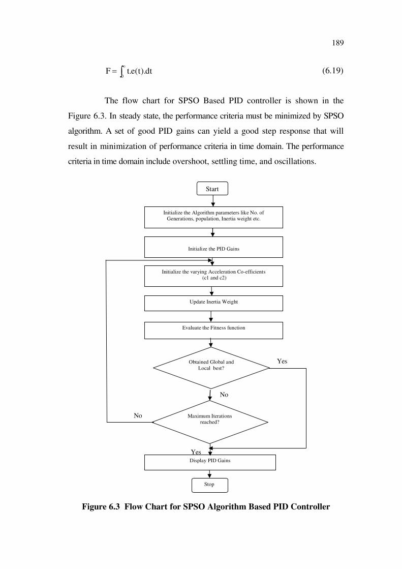
The flow chart for SPSO Based PID controller is shown in the

Figure 6.3. In steady state, the performance criteria must be minimized by SPSO

algorithm. A set of good PID gains can yield a good step response that will

result in minimization of performance criteria in time domain. The performance

criteria in time domain include overshoot, settling time, and oscillations.

Figure 6.3 Flow Chart for SPSO Algorithm Based PID Controller

190

6.2.4 Fuzzy Particle Swarm Optimization (FPSO)

Fuzzy-Particle Swarm Optimization is an Hybrid Evolutionary

Computation Based search algorithm which can be used to solve optimization

problems. In this technique, Fuzzy logic is used to dynamically adapt the

inertia weight of the PSO. By linearly decreasing the inertia weight from

relatively large value to a small value through the course of a PSO run, PSO

tends to have more global search ability at the beginning of the run while

local search ability at the end of the run (Shi and Eberhert 2001). As a result,

a deterministic approach towards the optimal gain value of the PID Controller

is obtained. In the proposed FPSO method, the inertia weight factor, W is

varied according to the mathematical model representing the application.

Modify the member velocity of each individual according to the inertia

weight factor w which is obtained from fuzzy logic. In order to fuzzify the

variation of factor W, two fuzzy inputs are used. The first input is called

Current Best Performance Evaluation (CBFE) and describes the point that has

the best performance. In this technique, the Normalized form of Current Best

Performance Evaluation (NCPBE) is calculated using the Equation (6.20).

CBPEmin is the best acceptable performance of FPSO and CBPEmax is the

worst acceptable performance of FPSO. The second fuzzy input is the current

value of the inertia weight factor (Shi and Eberhert 2000).

minmax

min

CBPECBPE

CBPECBPENCBPE (6.20)

To design a fuzzy system to dynamically adapt the inertia weight,

normally the inputs to the system are variables that measure the performance

of the PSO and the output is the inertia weight or the variation of the inertia

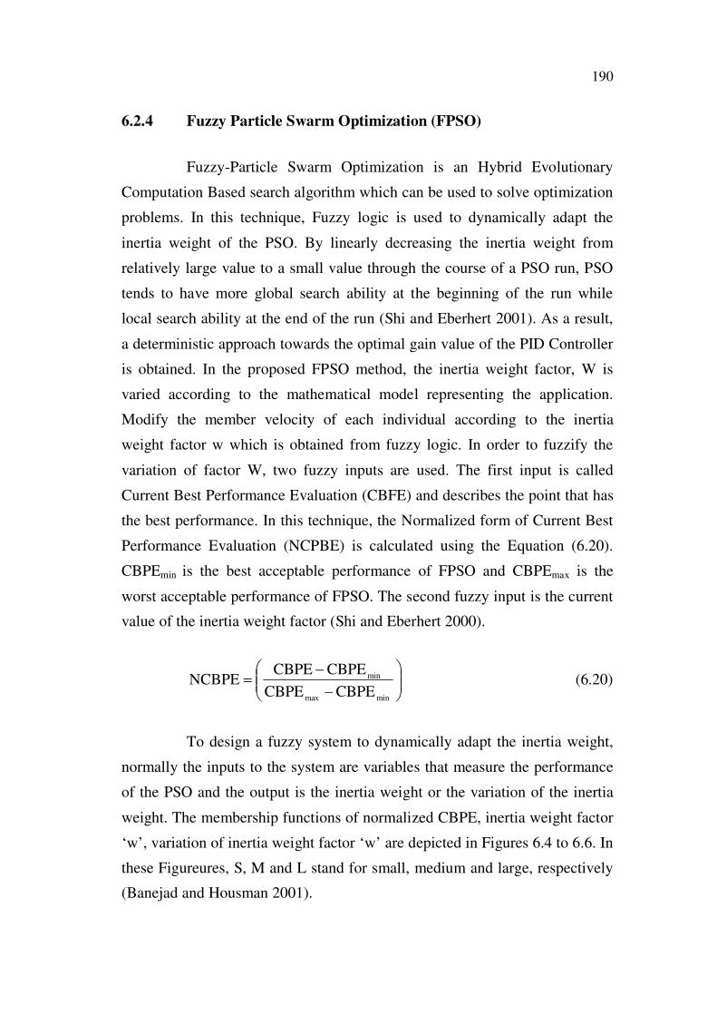
weight. The membership functions of normalized CBPE, inertia weight factor

‘w’, variation of inertia weight factor ‘w’ are depicted in Figures 6.4 to 6.6. In

these Figureures, S, M and L stand for small, medium and large, respectively

(Banejad and Housman 2001).

191

Figure 6.4 The Membership Function of the Normalized CBPE

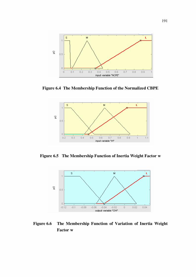
Figure 6.5 The Membership Function of Inertia Weight Factor w

Figure 6.6 The Membership Function of Variation of Inertia Weight

Factor w

192

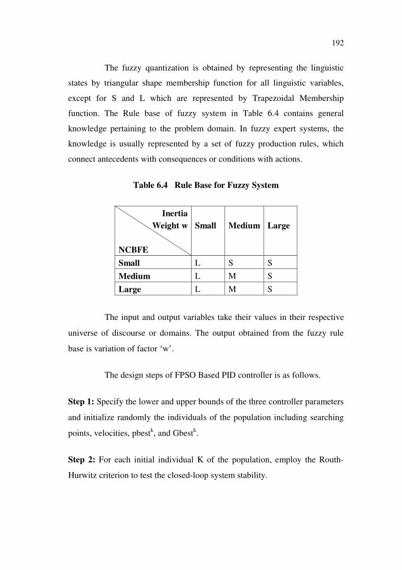
The fuzzy quantization is obtained by representing the linguistic

states by triangular shape membership function for all linguistic variables,

except for S and L which are represented by Trapezoidal Membership

function. The Rule base of fuzzy system in Table 6.4 contains general

knowledge pertaining to the problem domain. In fuzzy expert systems, the

knowledge is usually represented by a set of fuzzy production rules, which

connect antecedents with consequences or conditions with actions.

Table 6.4 Rule Base for Fuzzy System

Inertia

Weight w

NCBFE

Small Medium Large

Small L S S

Medium L M S

Large L M S

The input and output variables take their values in their respective

universe of discourse or domains. The output obtained from the fuzzy rule

base is variation of factor ‘w’.

The design steps of FPSO Based PID controller is as follows.

Step 1: Specify the lower and upper bounds of the three controller parameters

and initialize randomly the individuals of the population including searching

points, velocities, pbestk, and Gbest

k.

Step 2: For each initial individual K of the population, employ the Routh-

Hurwitz criterion to test the closed-loop system stability.

193

Step 3: Generate position of the particle randomly.

Step 4: Calculate the fitness function value of each individual in the

population using the evaluation function ‘f’ given by Equation (6.24).

Step 5: Compare each individual’s evaluation value with its pbestk. The best

fitness value denoted as Gbestk

Step 6: Update the velocity of particle in each individual ‘k’ with the inertia

weight factor ‘W’ obtained from fuzzy logic.

)xgbest(*()2rand*1Cxpbest(*()1rand*1CwVVk

g,jg,i

k

g,jg,i

k

j

1k

j(6.21)

1k

j

k

g,j

1k

g,j vxx (6.23)

Step 7: Update local best Pi and global best Pg by using the fitness function in

Equation (6.24).

Step 8: If the number of iterations reaches the maximum, then go to Step 9

Otherwise, go to Step 2.

Step 9: The individual that generates the latest is an optimal controller

parameter.

The variables used in the FPSO algorithm is tabulated in Table 6.4

194

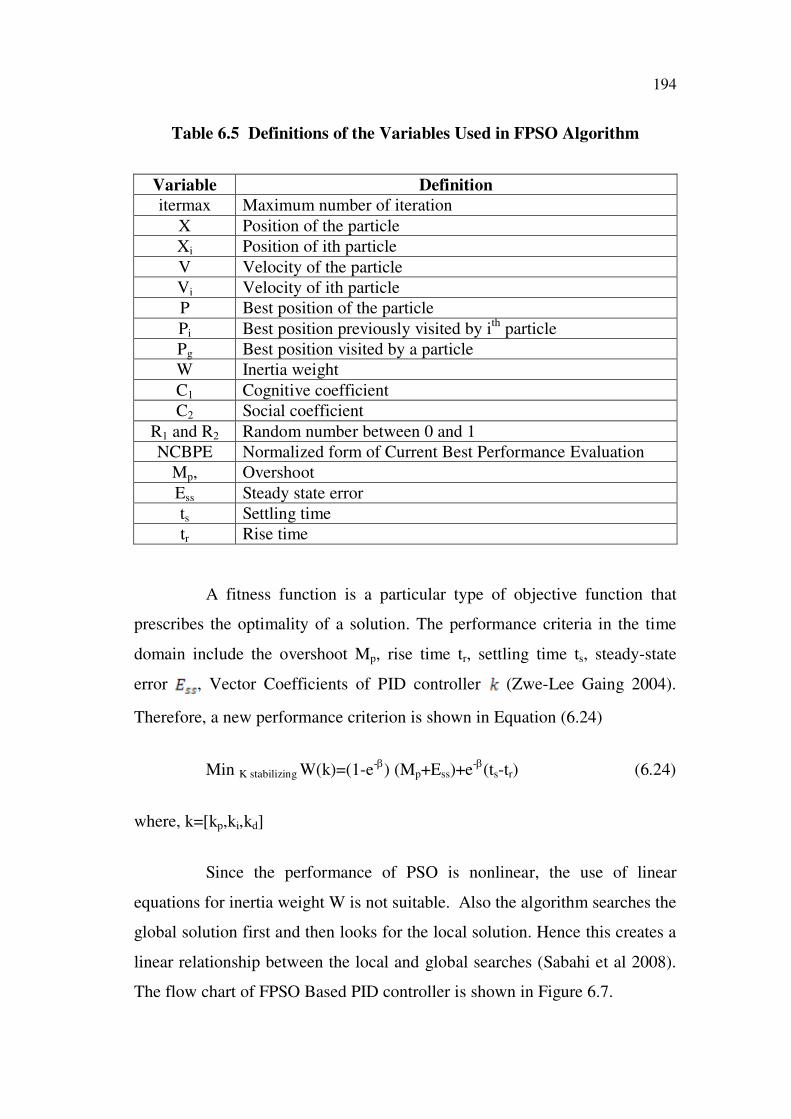
Table 6.5 Definitions of the Variables Used in FPSO Algorithm

Variable Definition

itermax Maximum number of iteration

X Position of the particle

Xi Position of ith particle

V Velocity of the particle

Vi Velocity of ith particle

P Best position of the particle

Pi Best position previously visited by ith

particle

Pg Best position visited by a particle

W Inertia weight

C1 Cognitive coefficient

C2 Social coefficient

R1 and R2 Random number between 0 and 1

NCBPE Normalized form of Current Best Performance Evaluation

Mp, Overshoot

Ess Steady state error

ts Settling time

tr Rise time

A fitness function is a particular type of objective function that

prescribes the optimality of a solution. The performance criteria in the time

domain include the overshoot Mp, rise time tr, settling time ts, steady-state

error , Vector Coefficients of PID controller (Zwe-Lee Gaing 2004).

Therefore, a new performance criterion is shown in Equation (6.24)

Min K stabilizing W(k)=(1-e-

) (Mp+Ess)+e-

(ts-tr) (6.24)

where, k=[kp,ki,kd]

Since the performance of PSO is nonlinear, the use of linear

equations for inertia weight W is not suitable. Also the algorithm searches the

global solution first and then looks for the local solution. Hence this creates a

linear relationship between the local and global searches (Sabahi et al 2008).

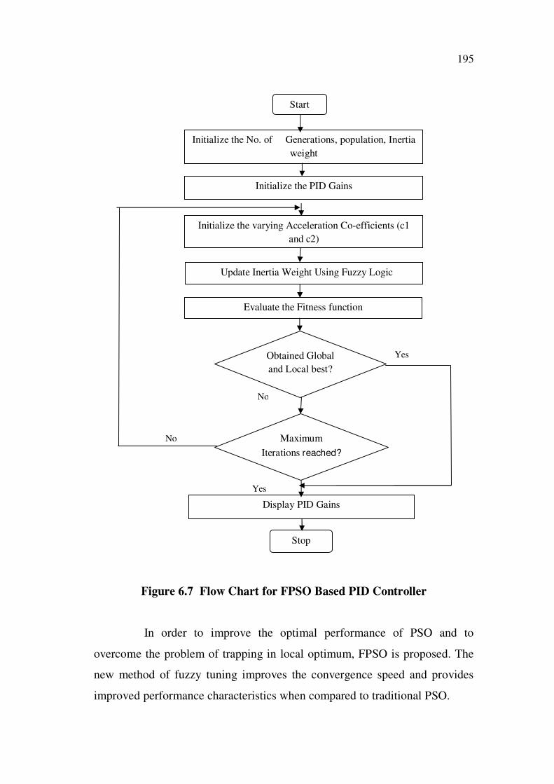
The flow chart of FPSO Based PID controller is shown in Figure 6.7.

195

Start

Initialize the No. of Generations, population, Inertia

weight

Initialize the PID Gains

Initialize the varying Acceleration Co-efficients (c1

and c2)

Display PID Gains

Evaluate the Fitness function

Update Inertia Weight Using Fuzzy Logic

Obtained Global

and Local best?

Maximum

Iterations reached?

Stop

No

Yes

Yes

No

Figure 6.7 Flow Chart for FPSO Based PID Controller

In order to improve the optimal performance of PSO and to

overcome the problem of trapping in local optimum, FPSO is proposed. The

new method of fuzzy tuning improves the convergence speed and provides

improved performance characteristics when compared to traditional PSO.

196

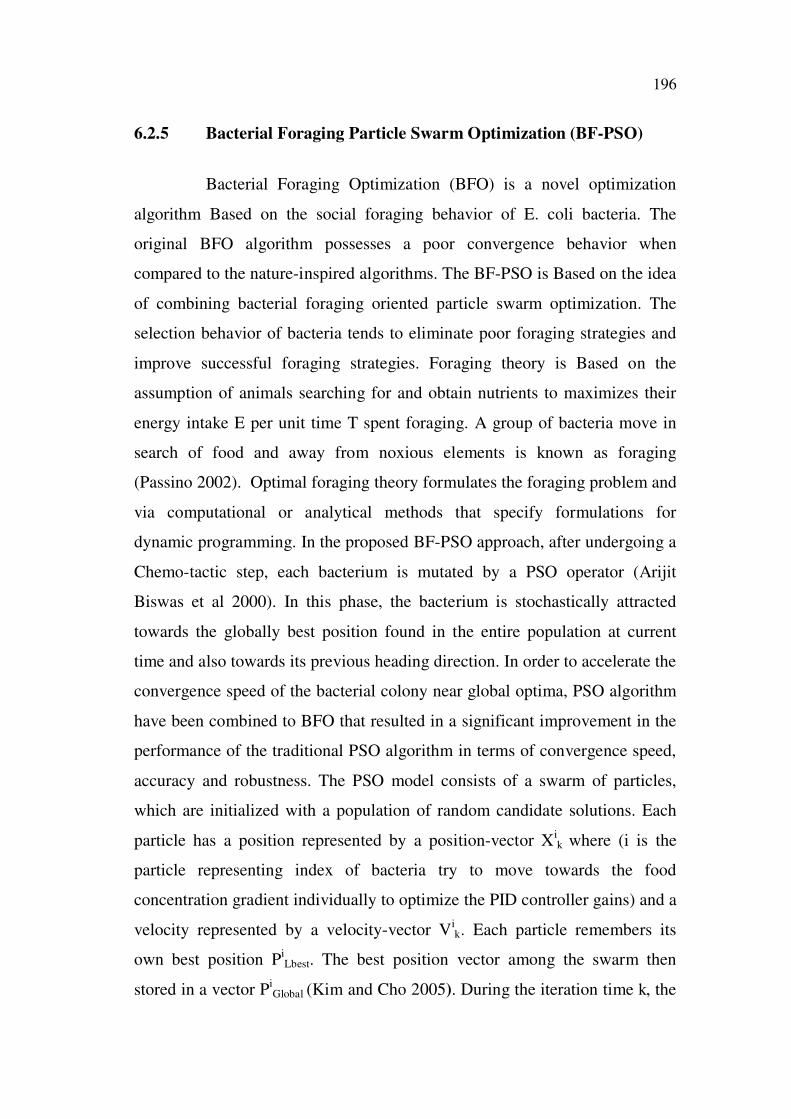
6.2.5 Bacterial Foraging Particle Swarm Optimization (BF-PSO)

Bacterial Foraging Optimization (BFO) is a novel optimization

algorithm Based on the social foraging behavior of E. coli bacteria. The

original BFO algorithm possesses a poor convergence behavior when

compared to the nature-inspired algorithms. The BF-PSO is Based on the idea

of combining bacterial foraging oriented particle swarm optimization. The

selection behavior of bacteria tends to eliminate poor foraging strategies and

improve successful foraging strategies. Foraging theory is Based on the

assumption of animals searching for and obtain nutrients to maximizes their

energy intake E per unit time T spent foraging. A group of bacteria move in

search of food and away from noxious elements is known as foraging

(Passino 2002). Optimal foraging theory formulates the foraging problem and

via computational or analytical methods that specify formulations for

dynamic programming. In the proposed BF-PSO approach, after undergoing a

Chemo-tactic step, each bacterium is mutated by a PSO operator (Arijit

Biswas et al 2000). In this phase, the bacterium is stochastically attracted

towards the globally best position found in the entire population at current

time and also towards its previous heading direction. In order to accelerate the

convergence speed of the bacterial colony near global optima, PSO algorithm

have been combined to BFO that resulted in a significant improvement in the

performance of the traditional PSO algorithm in terms of convergence speed,

accuracy and robustness. The PSO model consists of a swarm of particles,

which are initialized with a population of random candidate solutions. Each

particle has a position represented by a position-vector Xik where (i is the

particle representing index of bacteria try to move towards the food

concentration gradient individually to optimize the PID controller gains) and a

velocity represented by a velocity-vector Vik. Each particle remembers its

own best position PiLbest. The best position vector among the swarm then

stored in a vector PiGlobal (Kim and Cho 2005). During the iteration time k, the

197

new velocity is updated Based on the previous velocity as mentioned in

Equation (6.25).

Vid = W*Vid + C1R1 (Pid – Xid) + C2R2 (Pgd– Xid) (6.25)

The new position is then determined by the sum of the previous

position and the new velocity as shown in Equation (6.26). The movement of

the particle is decided by the memory of its best past position and the

experience of the most successful particle in the swarm.

Xid(new)=xid(old)+Vid (6.26)

In this algorithm explained below, ‘N’ denotes the number of

bacteria, ‘k’ denotes the no.of reproduction loops, and ‘ell’ denotes the

number of elimination dispersal.

Step 1: First initialize the parameters like number of bacteria S, Maximum

number of swim length Ns, Chemotactic steps Nc, The number of

reproduction steps Nre, Elimination and dispersal events Ned, Ped Cognitive

coefficient C1 and Social coefficient C2, and random numbers R1and R2.

Step 2: The values of Kp, Ki, Kd are initialized randomly within the optimal

range of values for each gains.

Step 3: Generate the random direction (n,i) and position P(i,j), dimension of

search space ‘n’, elimination and dispersal limit ‘l’ and ‘k’ is the

reproduction.

Step 4: ‘l’ is incremented by one for every cycle until it reaches the

elimination and dispersal limit l = l +1

198

Step 5: ‘k’is incremented by one for every cycle until it reaches the

Reproduction limit.

Step 6: Chemotaxis loop: j=j+1 for i=1,2,….,S, compute the fitness of J

(i,j,k,l),

J(i,j,k,l) = Fitness (p(i,j,k,l)) (6.27)

Store the best fitness function in Jlast as in Equation (6.28) and the

best fitness function for each bacteria will be selected to be the local best

Jlocal as in Equation (6.29).

Jlast(i,j,k,l) = Jlast(i,j,k,l) (6.28)

Jlocal(i,j,k,l) = Jlast(i,j,k,l) (6.29)

Update the Position and fitness function of the bacteria as given in

Equation (6.30) and allow the bacteria to swim in right direction and store the

bacteria into Jlast using Equation (6.31).

P(i,j+1)=p(i,j)+c(i)* (n,i) (6.30)

Jlast=(i,j+1,k,l) (6.31)

Store the Jlast and update the position of the bacteria using fitness

function

P(i,j+1,k,l)=p(i,j,k,l)+c(i)* (n,i) (6.32)

Step 7: Evaluate the local best position Pl(best) in Equation (6.33) and global

best position Pg(best) in Equation (6.34) for each bacterium.

199

Pcurrent(i,j+1)=p(i,j+1) (6.33)

Jlocal(i,j+1)jlast(i,j+1) (6.34)

Step 8: Update position and velocity of the dth coordinate of the ith bacterium

according to the Equations (6.35) and (6.36)

Vid=w*vid+c1Ri(Plbest-Pcurrent)+c2R2(Pgbest-Pcurrent) (6.35)

dnew

(i,j+1,k)= dold

(I,j+1,k)+ (6.36)

Step 9: In Reproduction, for the given k and l, and for each i = 1, 2,. . . ,N,

the health of the bacterium ‘i’ is obtained as in Equation (6.37)

Jhealth=sum(J(i,j,k,l) (6.37)

Sort bacteria and chemotactic parameters C(i) in order of ascending

cost Jhealth (higher cost means lower health).

Substep: The Sr bacteria with the highest Jhealth values die and the remaining

Sr bacteria with the best values split (this process is performed by the copies

that are made are placed at the same location as their parent) into i and i +Sr

as given by Equation (6.38).

P(i+Sr,j,k+1,l)=p(i,j,k+1,l) (6.38)

Step 10: If k<Nre go to step 5. (In case, if the specified number of

reproduction is not reached, start the next generation in chemo-taxis until the

best solution is obtained).

Step 12: Elimination–dispersal: For i = 1,2,. . . ,N, with probability Ped,

eliminate and disperse each bacterium, which results in keeping the number of

bacteria in the population constant. To do this, if a bacterium is eliminated,

200

simply disperse one to a random location on the optimization domain.

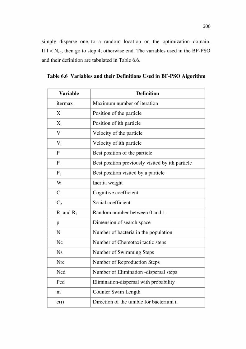
If l < Ned, then go to step 4; otherwise end. The variables used in the BF-PSO

and their definition are tabulated in Table 6.6.

Table 6.6 Variables and their Definitions Used in BF-PSO Algorithm

Variable Definition

itermax Maximum number of iteration

X Position of the particle

Xi Position of ith particle

V Velocity of the particle

Vi Velocity of ith particle

P Best position of the particle

Pi Best position previously visited by ith particle

Pg Best position visited by a particle

W Inertia weight

C1 Cognitive coefficient

C2 Social coefficient

R1 and R2 Random number between 0 and 1

p Dimension of search space

N Number of bacteria in the population

Nc Number of Chemotaxi tactic steps

Ns Number of Swimming Steps

Nre Number of Reproduction Steps

Ned Number of Elimination -dispersal steps

Ped Elimination-dispersal with probability

m Counter Swim Length

c(i) Direction of the tumble for bacterium i.

201

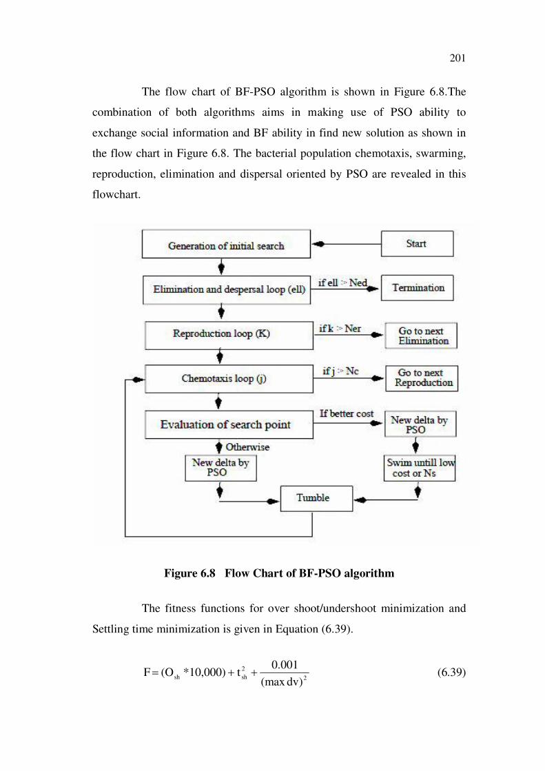
The flow chart of BF-PSO algorithm is shown in Figure 6.8.The

combination of both algorithms aims in making use of PSO ability to

exchange social information and BF ability in find new solution as shown in

the flow chart in Figure 6.8. The bacterial population chemotaxis, swarming,

reproduction, elimination and dispersal oriented by PSO are revealed in this

flowchart.

Figure 6.8 Flow Chart of BF-PSO algorithm

The fitness functions for over shoot/undershoot minimization and

Settling time minimization is given in Equation (6.39).

2

2

shsh)dv(max

001.0t10,000)*(OF (6.39)

202

where, Osh is overshoot, 2

sht is settling time and maxdv is maximum deviation.

Minimization of F corresponds to a minimum overshoot (Osh), minimum

settling time (tsh), and maximum deviation (max dv). Hence, a set of good

control parameters Kp, Ki, Kd is generated and yields a good response that will

result in performance criteria minimization in the time domain (Korani et al

2008).

6.2.6 Hybrid Genetic Algorithm (HGA)

Recent surveys of GA, relating to improvements in the search

process with respect to control system engineering problems can be found in

(Michalewicz 1999) (Tsutsui and Goldberg 2002) (Yoshida et al 2000). Inter-

mixing the salient features of the algorithms may be found to be more

effective in specific application areas like power system operation and

control. Recently, hybridization of the evolutionary algorithm is getting

popular due to their capabilities in handling several real world problems

involving complexity, noisy environment, imprecision, uncertainty, and

vagueness (Grosan and Abraham 2007). Even though EA belongs to the same

basic skeleton called Evolution Strategies, it is differentiated by the way the

hybridization of the algorithm is developed. These optimization models could

provide a social foraging environment where groups of parameters

communicate cooperatively for finding solutions to engineering problems

(Kim and Cho 2006). HGA is most suitable for parameter optimization

problem, particularly when the control structure is provided. A typical task of

Hybrid-GA is to find the best values of a predefined set of control parameters

associated with process model. The major advantages of HGA are capability

enhancement, improved quality and efficiency in reaching the global solution.

The steps involved in Hybrid Genetic Algorithm are as follows:

203

Step 1 Initialize the parameters like number of bacteria in the population S,

Maximum number of swim length Ns, Chemotactic steps Nc, The number of

reproduction steps Nre, Elimination-dispersal events Ned, Elimination-

dispersal with probability Ped .

Step 2: Evaluate all the chromosomes according to the fitness function in

Equation (6.46. The fitness function exactly fits the problem of the solution

space and the chromosome. The best fitness value is kept as the best solution

set.

Step 3: In the chemotactic process, the bacteria climb the nutrient

concentration, avoid noxious substances, and search for a way out of neutral

media. The bacterium usually takes a tumble followed by a run. For Nc the

direction of movement after a tumble is given in Equation (6.40).

)i()i(

)i()i(C)k,lj,i()k,lj,i(

T(6.40)

If the cost at i(j+1,k,l) is better than the cost at (i,j,k,l) then the

bacterium takes another step of size C(i) in that direction. This process will be

continued until the number of steps taken is not greater than Ns.

Step 4: After evaluating chemotaxis the bacteria climb the swarming,

Bacteria in times of stresses release attractants to signal bacteria to swarm

together. It, however, also releases a repellant to signal others to be at a

minimum distance from it. Thus all of them will have a cell to cell attraction

via attractant and cell to cell repulsion via repellant as in Equation ( 6.40).

Step 5: In the selection process, part of the chromosomes will be eliminated

and remaining chromosomes will be selected.

204

Step 6: The crossover operator produces two off springs (new candidate

solutions) by recombining the information from two parents is given in

Equation (6.41) and Equation (6.42).

ju

x

u

jx1x~

jv (6.41)

jv

x

v

jx1x~

ju (6.42)

Step 7: In mutation rate, several chromosomes will be selected from the

population, and then randomly change the value of parts of the dimensions.

This will give the population a larger chance to generate new species. For

optimization, it is chance to get an abrupt evolution shown in Equation (6.43).

0),xx~,k(x~0),x~x,k(x~

x)L(

jjj

j

)U(

jj

j(6.43)

Step 8: After the mutation steps have been covered, a reproduction step takes

place. The fitness (accumulated cost) of the bacteria is sorted in ascending

order. Sr (Sr=S/2) bacteria having higher fitness die and the remaining Sr is

allowed to split into two thus keeping the population size constant which is

given by ITSEihealth in Equation ( 6.44).

1N

1j

i

health

c

)l,k,j,i(ITSEITSE (6.44)

let i=1,2…N be the health of the bacterium i. The Sr bacteria with the highest

ITSEhealth values die and the remaining Sr bacteria with the best values will

split.

Step 9: The steps 2 to 6 are repeated until the maximum iteration is reached,

else go to step 3 and start the next generation of the chemotactic loop.

205

Step 10: Elimination–dispersal: For i = 1,2,. . . , N, with probability Ped,

eliminate and disperse each bacterium, which results in keeping the number of

bacteria in the population constant. When an individual is eliminated, the

course does not generate another one via the initialization process, but it

generates a new individual via mutating all the dimensions from the

eliminated one. If l < Ned, then go to (step 3); otherwise, end. The variables

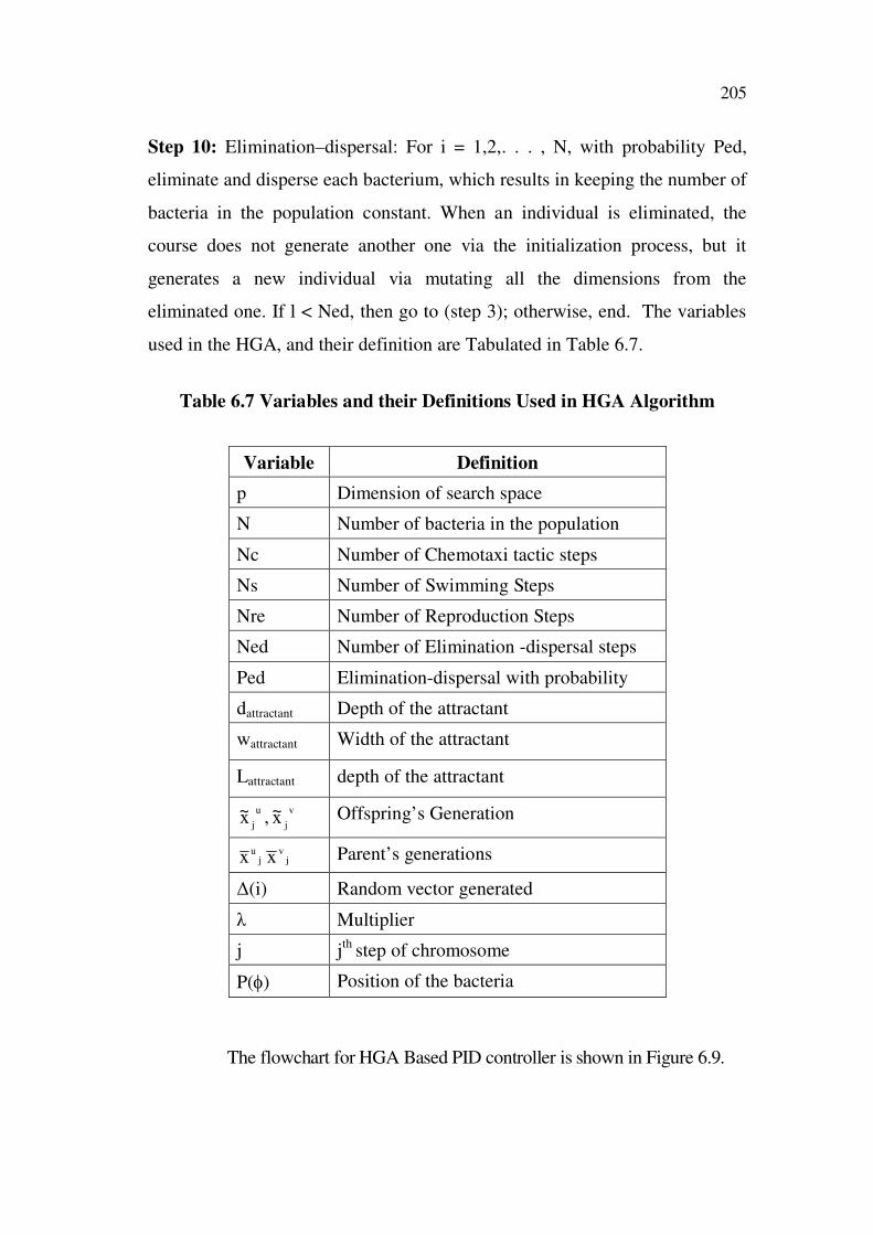
used in the HGA, and their definition are Tabulated in Table 6.7.

Table 6.7 Variables and their Definitions Used in HGA Algorithm

Variable Definition

p Dimension of search space

N Number of bacteria in the population

Nc Number of Chemotaxi tactic steps

Ns Number of Swimming Steps

Nre Number of Reproduction Steps

Ned Number of Elimination -dispersal steps

Ped Elimination-dispersal with probability

dattractant Depth of the attractant

wattractant Width of the attractant

Lattractant depth of the attractant

u

jx~ ,

v

jx~ Offspring’s Generation

jux j

vx Parent’s generations

(i) Random vector generated

Multiplier

j jth

step of chromosome

P( ) Position of the bacteria

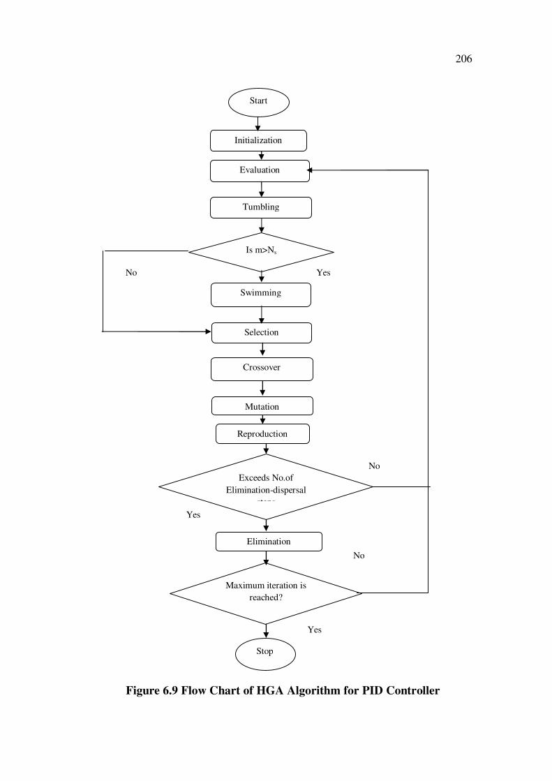
The flowchart for HGA Based PID controller is shown in Figure 6.9.

206

Start

Initialization

Evaluation

Tumbling

Is m>Ns

Crossover

Mutation

Swimming

Selection

Reproduction

Elimination

Exceeds No.of

Elimination-dispersal

steps

Maximum iteration is

reached?

Stop

Yes

No

No

Yes

No

Yes

Figure 6.9 Flow Chart of HGA Algorithm for PID Controller

207

The fitness function for HGA is defined in Equation (6.45). The

objective function measures the performance of the system. The fitness

function for HGA is defined as the Integral of Time multiplied by the

Absolute value of Error (ITAE) of the corresponding system. Therefore, it

becomes an unconstrained optimization problem to find a set of decision

variables by minimizing the objective function. The fitness of each particle is

evaluated using the ITAE fitness function as in Equation (6.45).

ess

)M)tmax(

ts(e

)k,k,k(Fmin

0

dip (6.45)

where,

=(1-e- )*|1-tr/max(t)| (6.46)

Kp, Ki, Kd is the optimal gains of PID controller, is the weighting factor,

Mo is the overshoot, ts settling time, ess is the steady state error. If the

weighting factor increases, the rising time of the response curve is small and

when decreases, the rising time also decreases (Kim and Park 2005). The

advanced HGA proposed in this research for PID gain tuning has been better

searching speed than the original GA.

6.3 DESIGN OF EA BASED PID CONTROLLER

In Conventional PID controller, the gains are randomly selected by

trial and error method. In this research, EA finds the Proportional, Integral

and Derivative gains of the PID controller, and the values are transferred to

the PID controller. In these algorithms, the gains of PID controller are

searched in the feasible region of response until a determined objective

function is minimized. In design of EA Based controllers, it is desirable that

controlled system include suitable transient and steady state response. Hence,

208

the important characteristics of the system such as overshoot, settling time

and oscillations are improved. Based on the input parameters and on the

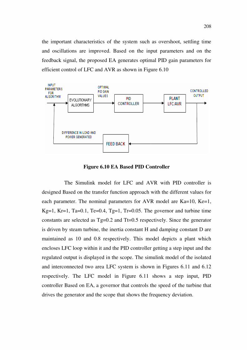
feedback signal, the proposed EA generates optimal PID gain parameters for

efficient control of LFC and AVR as shown in Figure 6.10

Figure 6.10 EA Based PID Controller

The Simulink model for LFC and AVR with PID controller is

designed Based on the transfer function approach with the different values for

each parameter. The nominal parameters for AVR model are Ka=10, Ke=1,

Kg=1, Kr=1, Ta=0.1, Te=0.4, Tg=1, Tr=0.05. The governor and turbine time

constants are selected as Tg=0.2 and Tt=0.5 respectively. Since the generator

is driven by steam turbine, the inertia constant H and damping constant D are

maintained as 10 and 0.8 respectively. This model depicts a plant which

encloses LFC loop within it and the PID controller getting a step input and the

regulated output is displayed in the scope. The simulink model of the isolated

and interconnected two area LFC system is shown in Figures 6.11 and 6.12

respectively. The LFC model in Figure 6.11 shows a step input, PID

controller Based on EA, a governor that controls the speed of the turbine that

drives the generator and the scope that shows the frequency deviation.

209

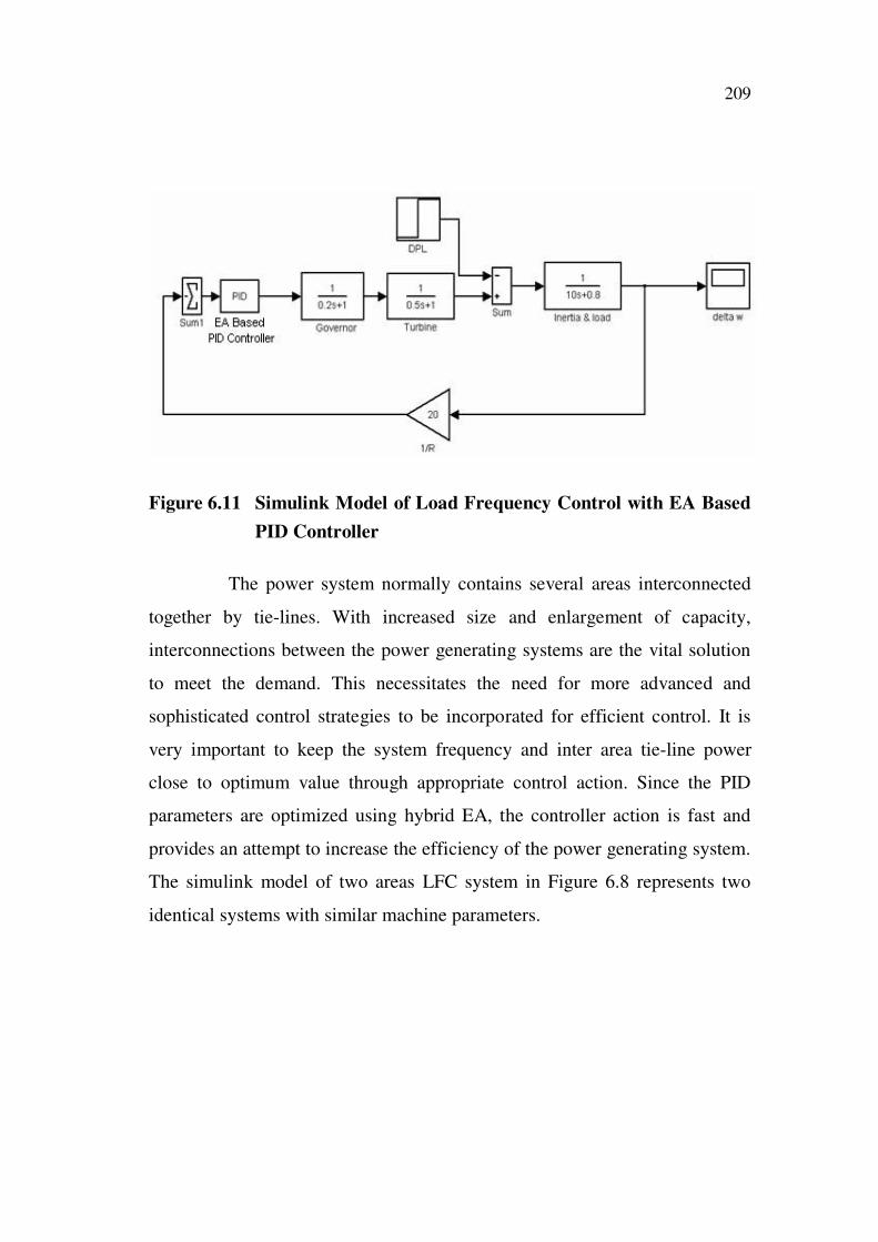
Figure 6.11 Simulink Model of Load Frequency Control with EA Based

PID Controller

The power system normally contains several areas interconnected

together by tie-lines. With increased size and enlargement of capacity,

interconnections between the power generating systems are the vital solution

to meet the demand. This necessitates the need for more advanced and

sophisticated control strategies to be incorporated for efficient control. It is

very important to keep the system frequency and inter area tie-line power

close to optimum value through appropriate control action. Since the PID

parameters are optimized using hybrid EA, the controller action is fast and

provides an attempt to increase the efficiency of the power generating system.

The simulink model of two areas LFC system in Figure 6.8 represents two

identical systems with similar machine parameters.

210

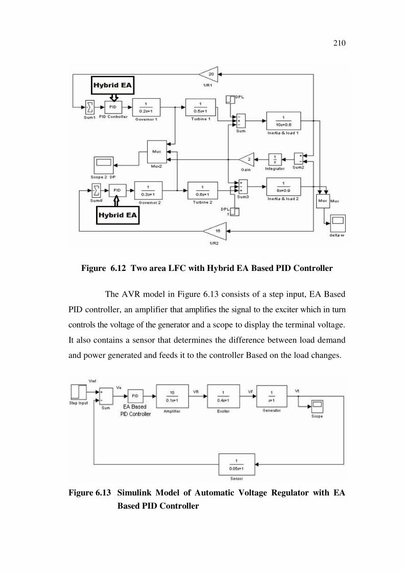
Figure 6.12 Two area LFC with Hybrid EA Based PID Controller

The AVR model in Figure 6.13 consists of a step input, EA Based

PID controller, an amplifier that amplifies the signal to the exciter which in turn

controls the voltage of the generator and a scope to display the terminal voltage.

It also contains a sensor that determines the difference between load demand

and power generated and feeds it to the controller Based on the load changes.

Figure 6.13 Simulink Model of Automatic Voltage Regulator with EA

Based PID Controller

211

6.4 SIMULATION RESULTS

The essential requirements of AGC are a continuous balance

between electrical power generation and a varying load demand, while

maintaining system frequency, voltage levels and the power grid security.

AGC is decentralized control operating in each control area to monitor the

frequency and voltage of a power generating system. LFC and AVR are

installed in each generator to maintain constant frequency and voltage under

different operating conditions. The effectiveness of the proposed hybrid EA is

evaluated and compared for damping the system oscillations during small and

large disturbances. The simulation results for Load Frequency Control (LFC)

and Automatic Voltage Regulator (AVR) are given for a single area system to

quantify the benefits of hybrid EA Based PID controllers. The simulation was

done using the Simulink package available in MATLAB R2008b. The LFC

and AVR were simulated on Intel core 2 Duo (2.4 GHz), 3GB RAM PC.

Simulink model for LFC and AVR with EA Based PID controller is

constructed Based on the transfer function model of the turbo alternator with

non-reheat type turbine. The Kp, KI and Kd values for the PID controller are

obtained by running the M-file that calls the fitness function to evaluate the

fitness of the solution. The simulation was performed for different load and

regulations, and the results are discussed in this section.

6.4.1 EPSO Based PID Controller

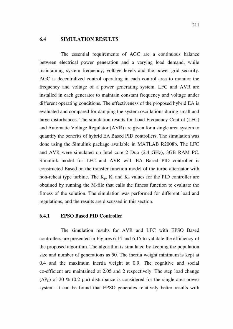
The simulation results for AVR and LFC with EPSO Based

controllers are presented in Figures 6.14 and 6.15 to validate the efficiency of

the proposed algorithm. The algorithm is simulated by keeping the population

size and number of generations as 50. The inertia weight minimum is kept at

0.4 and the maximum inertia weight at 0.9. The cognitive and social

co-efficient are maintained at 2.05 and 2 respectively. The step load change

PL) of 20 % (0.2 p.u) disturbance is considered for the single area power

system. It can be found that EPSO generates relatively better results with

212

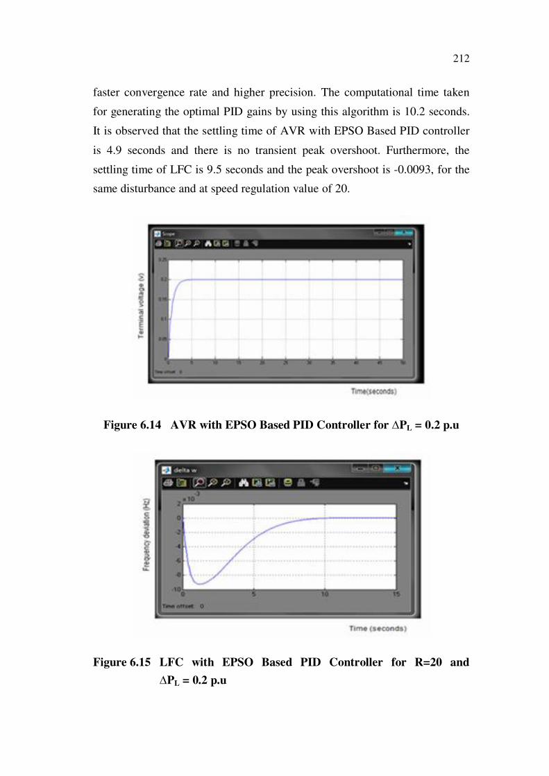
faster convergence rate and higher precision. The computational time taken

for generating the optimal PID gains by using this algorithm is 10.2 seconds.

It is observed that the settling time of AVR with EPSO Based PID controller

is 4.9 seconds and there is no transient peak overshoot. Furthermore, the

settling time of LFC is 9.5 seconds and the peak overshoot is -0.0093, for the

same disturbance and at speed regulation value of 20.

Figure 6.14 AVR with EPSO Based PID Controller for PL = 0.2 p.u

Figure 6.15 LFC with EPSO Based PID Controller for R=20 and

PL = 0.2 p.u

213

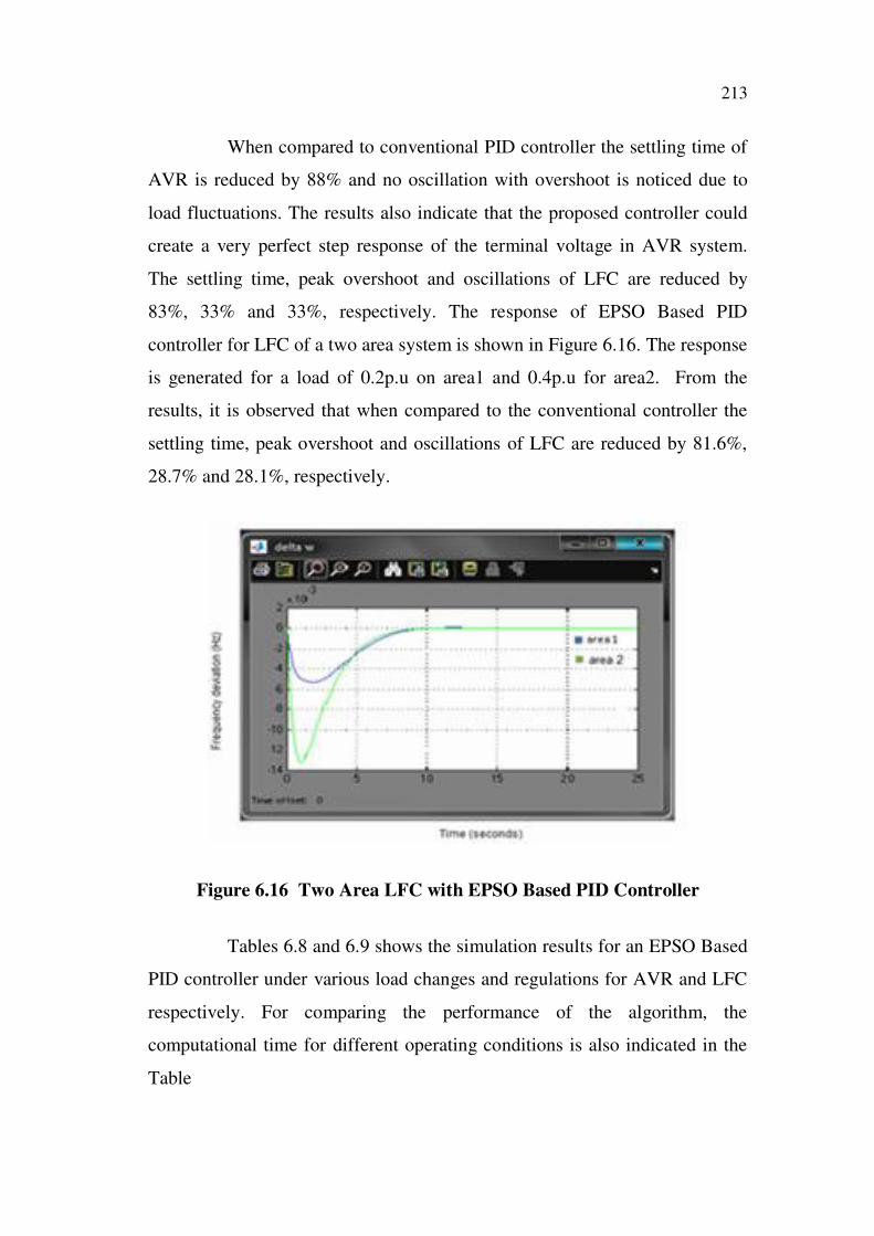
When compared to conventional PID controller the settling time of

AVR is reduced by 88% and no oscillation with overshoot is noticed due to

load fluctuations. The results also indicate that the proposed controller could

create a very perfect step response of the terminal voltage in AVR system.

The settling time, peak overshoot and oscillations of LFC are reduced by

83%, 33% and 33%, respectively. The response of EPSO Based PID

controller for LFC of a two area system is shown in Figure 6.16. The response

is generated for a load of 0.2p.u on area1 and 0.4p.u for area2. From the

results, it is observed that when compared to the conventional controller the

settling time, peak overshoot and oscillations of LFC are reduced by 81.6%,

28.7% and 28.1%, respectively.

Figure 6.16 Two Area LFC with EPSO Based PID Controller

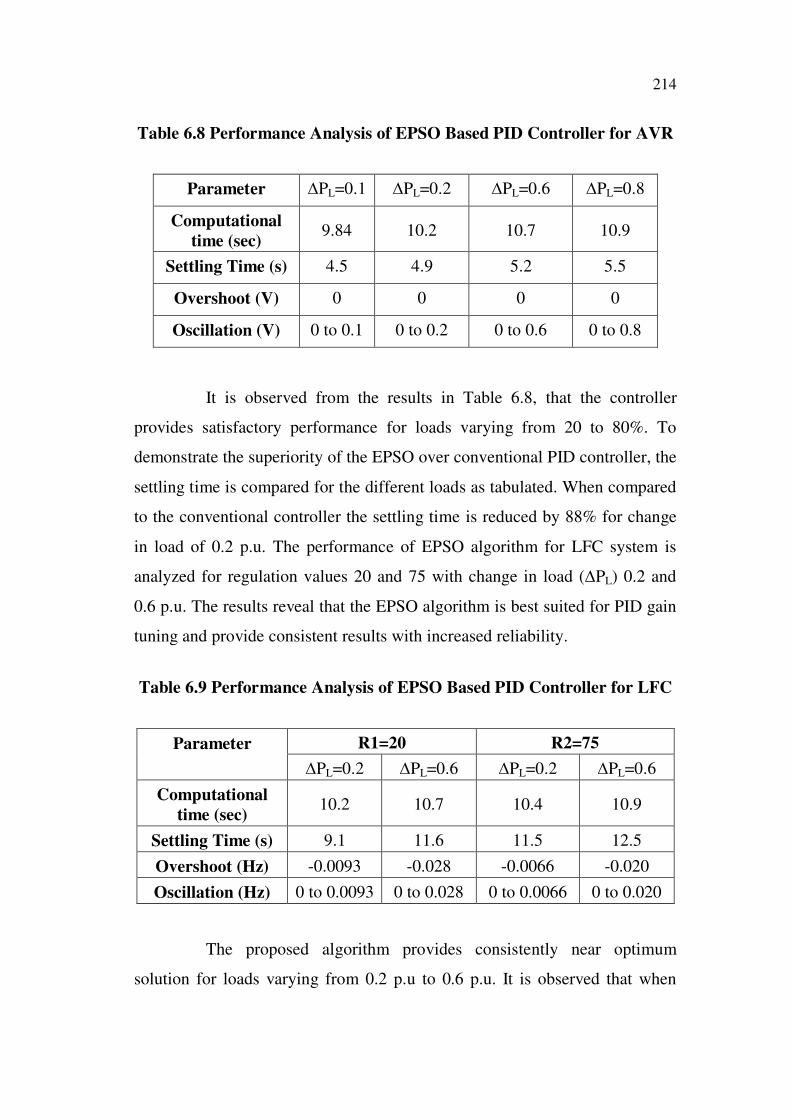
Tables 6.8 and 6.9 shows the simulation results for an EPSO Based

PID controller under various load changes and regulations for AVR and LFC

respectively. For comparing the performance of the algorithm, the

computational time for different operating conditions is also indicated in the

Table

214

Table 6.8 Performance Analysis of EPSO Based PID Controller for AVR

Parameter PL=0.1 PL=0.2 PL=0.6 PL=0.8

Computational

time (sec)9.84 10.2 10.7 10.9

Settling Time (s) 4.5 4.9 5.2 5.5

Overshoot (V) 0 0 0 0

Oscillation (V) 0 to 0.1 0 to 0.2 0 to 0.6 0 to 0.8

It is observed from the results in Table 6.8, that the controller

provides satisfactory performance for loads varying from 20 to 80%. To

demonstrate the superiority of the EPSO over conventional PID controller, the

settling time is compared for the different loads as tabulated. When compared

to the conventional controller the settling time is reduced by 88% for change

in load of 0.2 p.u. The performance of EPSO algorithm for LFC system is

analyzed for regulation values 20 and 75 with change in load ( PL) 0.2 and

0.6 p.u. The results reveal that the EPSO algorithm is best suited for PID gain

tuning and provide consistent results with increased reliability.

Table 6.9 Performance Analysis of EPSO Based PID Controller for LFC

R1=20 R2=75Parameter

PL=0.2 PL=0.6 PL=0.2 PL=0.6

Computational

time (sec)10.2 10.7 10.4 10.9

Settling Time (s) 9.1 11.6 11.5 12.5

Overshoot (Hz) -0.0093 -0.028 -0.0066 -0.020

Oscillation (Hz) 0 to 0.0093 0 to 0.028 0 to 0.0066 0 to 0.020

The proposed algorithm provides consistently near optimum

solution for loads varying from 0.2 p.u to 0.6 p.u. It is observed that when

215

compared to the conventional controller the settling time, peak overshoot and

oscillations of LFC are reduced by 83%, 33% and 33%, respectively for

regulation R as 75 with 20% increase in load.

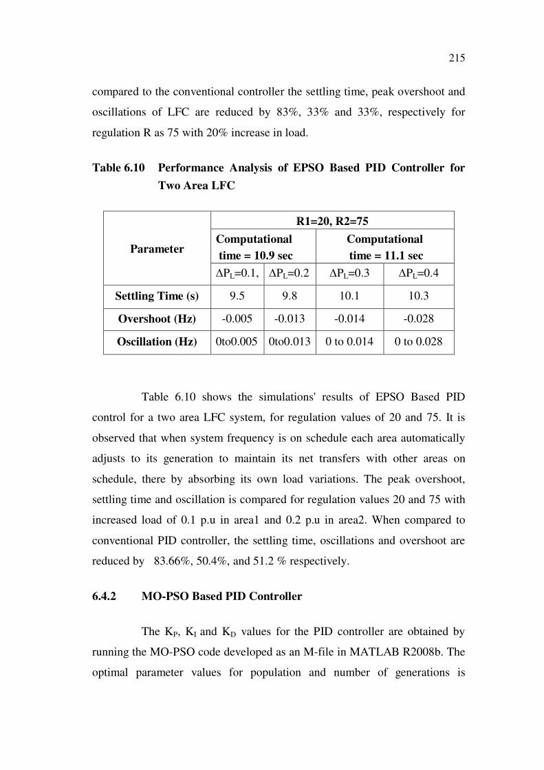
Table 6.10 Performance Analysis of EPSO Based PID Controller for

Two Area LFC

R1=20, R2=75

Computational

time = 10.9 sec

Computational

time = 11.1 secParameter

PL=0.1, PL=0.2 PL=0.3 PL=0.4

Settling Time (s) 9.5 9.8 10.1 10.3

Overshoot (Hz) -0.005 -0.013 -0.014 -0.028

Oscillation (Hz) 0to0.005 0to0.013 0 to 0.014 0 to 0.028

Table 6.10 shows the simulations' results of EPSO Based PID

control for a two area LFC system, for regulation values of 20 and 75. It is

observed that when system frequency is on schedule each area automatically

adjusts to its generation to maintain its net transfers with other areas on

schedule, there by absorbing its own load variations. The peak overshoot,

settling time and oscillation is compared for regulation values 20 and 75 with

increased load of 0.1 p.u in area1 and 0.2 p.u in area2. When compared to

conventional PID controller, the settling time, oscillations and overshoot are

reduced by 83.66%, 50.4%, and 51.2 % respectively.

6.4.2 MO-PSO Based PID Controller

The KP, KI and KD values for the PID controller are obtained by

running the MO-PSO code developed as an M-file in MATLAB R2008b. The

optimal parameter values for population and number of generations is

216

maintained at 50 and 25 for both LFC and AVR. The cognitive and social co-

efficient are maintained at 2.05 and 3 respectively. The PID gain values are

transferred to the AVR and LFC simulink model for simulating with different

load and regulation values. In proposed hybrid MO-PSO algorithm, the

objective functions are collectively minimized by assigning weight for

different objective functions. The computational time for the particle convergence

to the optimum values of PID gains in MO-PSO is 14.35 seconds for a change

in load of PL=0.1. In order demonstrate the stability of the algorithm the

computational time taken for convergence is tabulated in Tables 6.9 and 6.10.

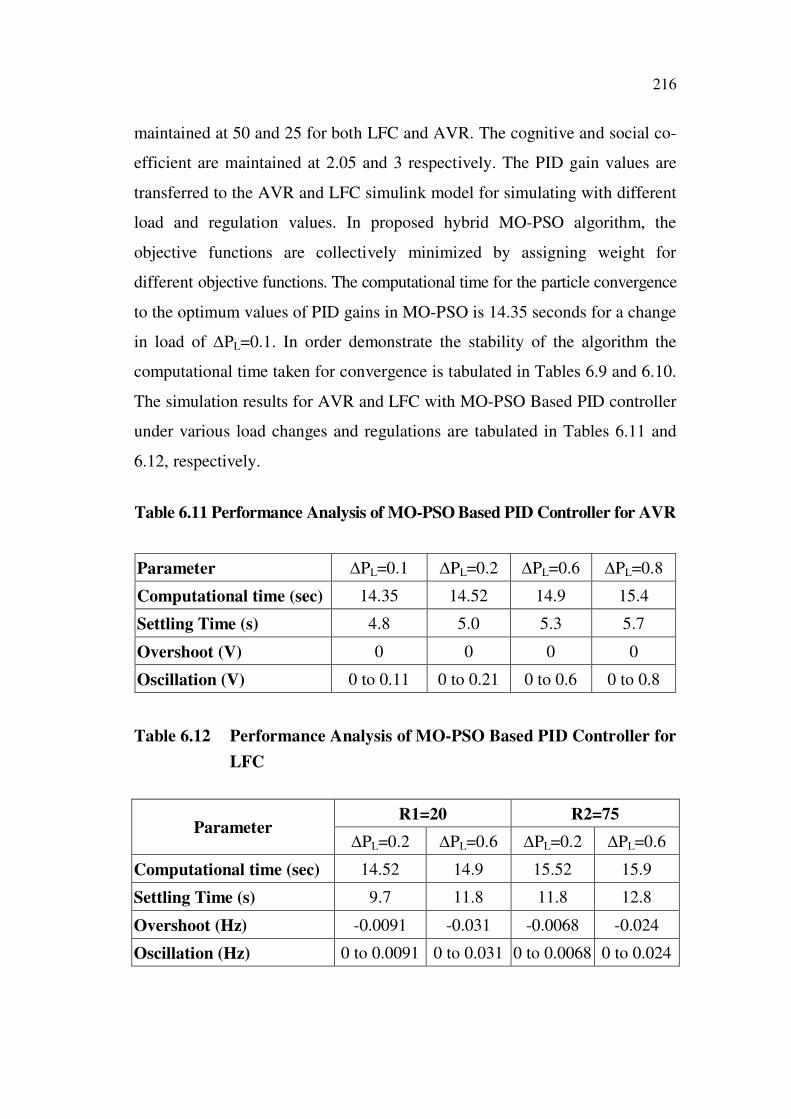
The simulation results for AVR and LFC with MO-PSO Based PID controller

under various load changes and regulations are tabulated in Tables 6.11 and

6.12, respectively.

Table 6.11 Performance Analysis of MO-PSO Based PID Controller for AVR

Parameter PL=0.1 PL=0.2 PL=0.6 PL=0.8

Computational time (sec) 14.35 14.52 14.9 15.4

Settling Time (s) 4.8 5.0 5.3 5.7

Overshoot (V) 0 0 0 0

Oscillation (V) 0 to 0.11 0 to 0.21 0 to 0.6 0 to 0.8

Table 6.12 Performance Analysis of MO-PSO Based PID Controller for

LFC

R1=20 R2=75Parameter

PL=0.2 PL=0.6 PL=0.2 PL=0.6

Computational time (sec) 14.52 14.9 15.52 15.9

Settling Time (s) 9.7 11.8 11.8 12.8

Overshoot (Hz) -0.0091 -0.031 -0.0068 -0.024

Oscillation (Hz) 0 to 0.0091 0 to 0.031 0 to 0.0068 0 to 0.024

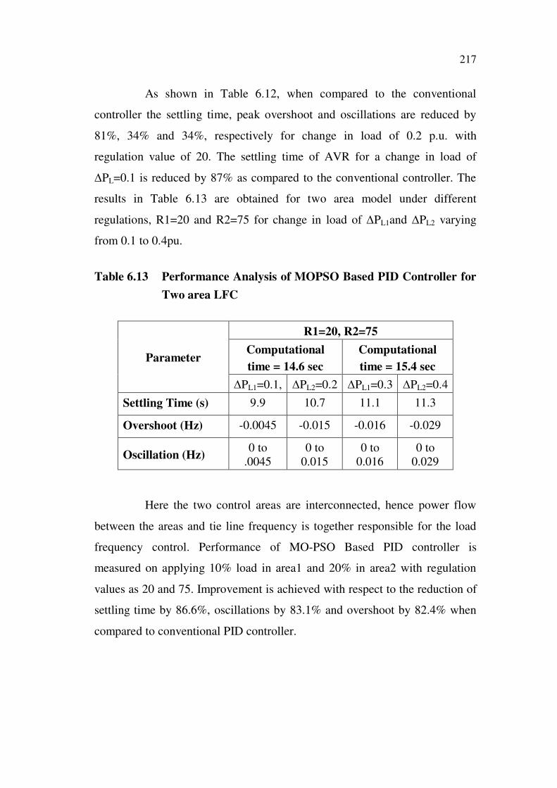
217

As shown in Table 6.12, when compared to the conventional

controller the settling time, peak overshoot and oscillations are reduced by

81%, 34% and 34%, respectively for change in load of 0.2 p.u. with

regulation value of 20. The settling time of AVR for a change in load of

PL=0.1 is reduced by 87% as compared to the conventional controller. The

results in Table 6.13 are obtained for two area model under different

regulations, R1=20 and R2=75 for change in load of PL1and PL2 varying

from 0.1 to 0.4pu.

Table 6.13 Performance Analysis of MOPSO Based PID Controller for

Two area LFC

R1=20, R2=75

Computational

time = 14.6 sec

Computational

time = 15.4 secParameter

PL1=0.1, PL2=0.2 PL1=0.3 PL2=0.4

Settling Time (s) 9.9 10.7 11.1 11.3

Overshoot (Hz) -0.0045 -0.015 -0.016 -0.029

Oscillation (Hz)0 to

.0045

0 to

0.015

0 to

0.016

0 to

0.029

Here the two control areas are interconnected, hence power flow

between the areas and tie line frequency is together responsible for the load

frequency control. Performance of MO-PSO Based PID controller is

measured on applying 10% load in area1 and 20% in area2 with regulation

values as 20 and 75. Improvement is achieved with respect to the reduction of

settling time by 86.6%, oscillations by 83.1% and overshoot by 82.4% when

compared to conventional PID controller.

218

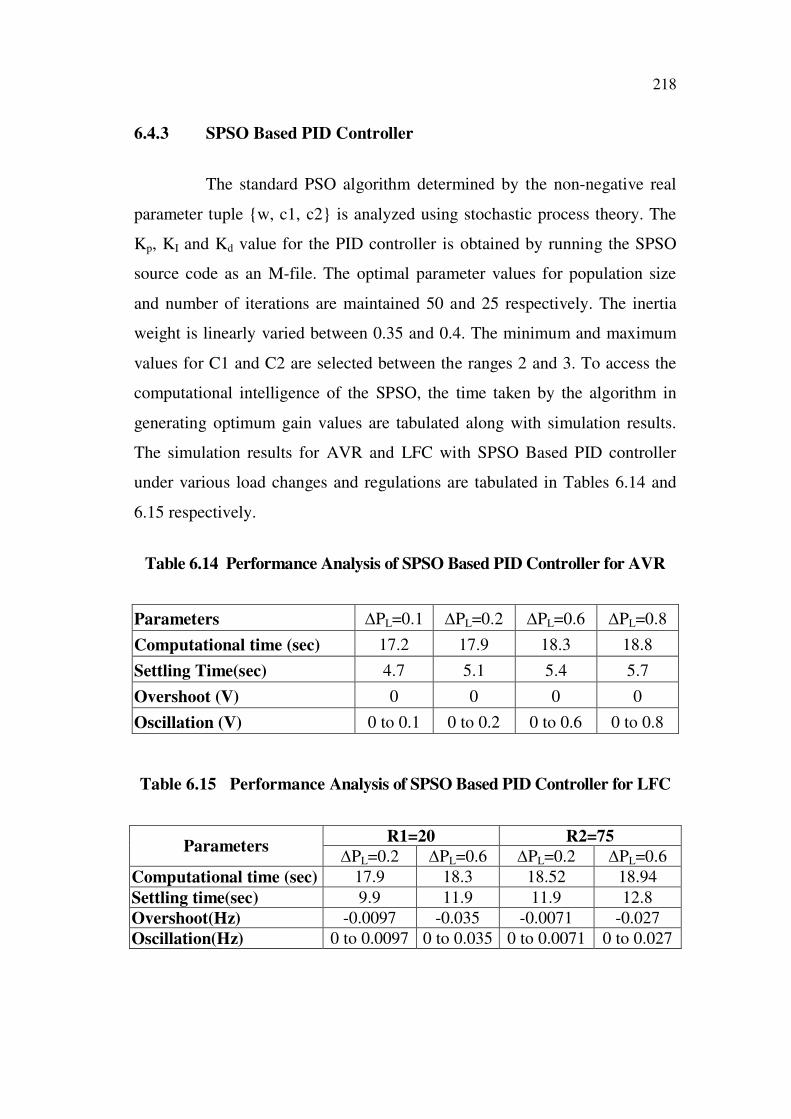
6.4.3 SPSO Based PID Controller

The standard PSO algorithm determined by the non-negative real

parameter tuple {w, c1, c2} is analyzed using stochastic process theory. The

Kp, KI and Kd value for the PID controller is obtained by running the SPSO

source code as an M-file. The optimal parameter values for population size

and number of iterations are maintained 50 and 25 respectively. The inertia

weight is linearly varied between 0.35 and 0.4. The minimum and maximum

values for C1 and C2 are selected between the ranges 2 and 3. To access the

computational intelligence of the SPSO, the time taken by the algorithm in

generating optimum gain values are tabulated along with simulation results.

The simulation results for AVR and LFC with SPSO Based PID controller

under various load changes and regulations are tabulated in Tables 6.14 and

6.15 respectively.

Table 6.14 Performance Analysis of SPSO Based PID Controller for AVR

Parameters PL=0.1 PL=0.2 PL=0.6 PL=0.8

Computational time (sec) 17.2 17.9 18.3 18.8

Settling Time(sec) 4.7 5.1 5.4 5.7

Overshoot (V) 0 0 0 0

Oscillation (V) 0 to 0.1 0 to 0.2 0 to 0.6 0 to 0.8

Table 6.15 Performance Analysis of SPSO Based PID Controller for LFC

R1=20 R2=75Parameters

PL=0.2 PL=0.6 PL=0.2 PL=0.6

Computational time (sec) 17.9 18.3 18.52 18.94

Settling time(sec) 9.9 11.9 11.9 12.8

Overshoot(Hz) -0.0097 -0.035 -0.0071 -0.027

Oscillation(Hz) 0 to 0.0097 0 to 0.035 0 to 0.0071 0 to 0.027

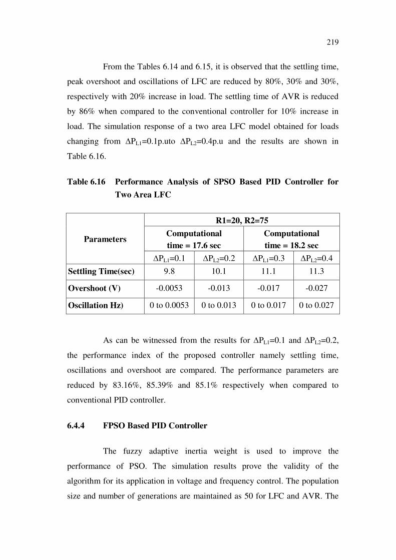
219

From the Tables 6.14 and 6.15, it is observed that the settling time,

peak overshoot and oscillations of LFC are reduced by 80%, 30% and 30%,

respectively with 20% increase in load. The settling time of AVR is reduced

by 86% when compared to the conventional controller for 10% increase in

load. The simulation response of a two area LFC model obtained for loads

changing from PL1=0.1p.uto PL2=0.4p.u and the results are shown in

Table 6.16.

Table 6.16 Performance Analysis of SPSO Based PID Controller for

Two Area LFC

R1=20, R2=75

Computational

time = 17.6 sec

Computational

time = 18.2 secParameters

PL1=0.1 PL2=0.2 PL1=0.3 PL2=0.4

Settling Time(sec) 9.8 10.1 11.1 11.3

Overshoot (V) -0.0053 -0.013 -0.017 -0.027

Oscillation Hz) 0 to 0.0053 0 to 0.013 0 to 0.017 0 to 0.027

As can be witnessed from the results for PL1=0.1 and PL2=0.2,

the performance index of the proposed controller namely settling time,

oscillations and overshoot are compared. The performance parameters are

reduced by 83.16%, 85.39% and 85.1% respectively when compared to

conventional PID controller.

6.4.4 FPSO Based PID Controller

The fuzzy adaptive inertia weight is used to improve the

performance of PSO. The simulation results prove the validity of the

algorithm for its application in voltage and frequency control. The population

size and number of generations are maintained as 50 for LFC and AVR. The

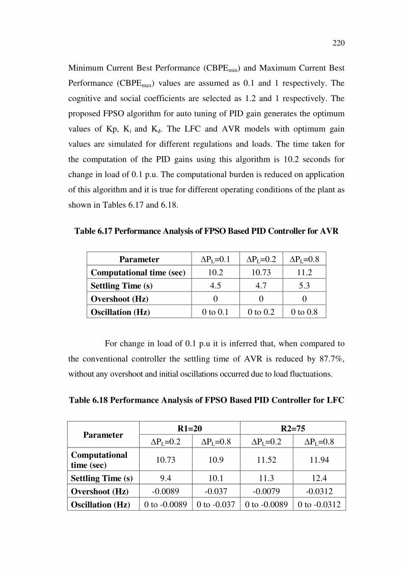
220

Minimum Current Best Performance (CBPEmin) and Maximum Current Best

Performance (CBPEmax) values are assumed as 0.1 and 1 respectively. The

cognitive and social coefficients are selected as 1.2 and 1 respectively. The

proposed FPSO algorithm for auto tuning of PID gain generates the optimum

values of Kp, Ki and Kd. The LFC and AVR models with optimum gain

values are simulated for different regulations and loads. The time taken for

the computation of the PID gains using this algorithm is 10.2 seconds for

change in load of 0.1 p.u. The computational burden is reduced on application

of this algorithm and it is true for different operating conditions of the plant as

shown in Tables 6.17 and 6.18.

Table 6.17 Performance Analysis of FPSO Based PID Controller for AVR

Parameter PL=0.1 PL=0.2 PL=0.8

Computational time (sec) 10.2 10.73 11.2

Settling Time (s) 4.5 4.7 5.3

Overshoot (Hz) 0 0 0

Oscillation (Hz) 0 to 0.1 0 to 0.2 0 to 0.8

For change in load of 0.1 p.u it is inferred that, when compared to

the conventional controller the settling time of AVR is reduced by 87.7%,

without any overshoot and initial oscillations occurred due to load fluctuations.

Table 6.18 Performance Analysis of FPSO Based PID Controller for LFC

R1=20 R2=75Parameter

PL=0.2 PL=0.8 PL=0.2 PL=0.8

Computational

time (sec)10.73 10.9 11.52 11.94

Settling Time (s) 9.4 10.1 11.3 12.4

Overshoot (Hz) -0.0089 -0.037 -0.0079 -0.0312

Oscillation (Hz) 0 to -0.0089 0 to -0.037 0 to -0.0089 0 to -0.0312

221

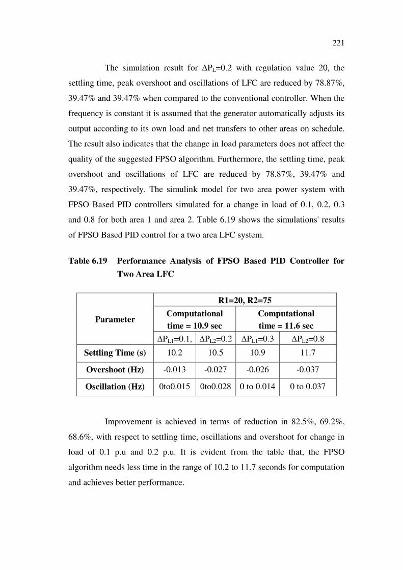
The simulation result for PL=0.2 with regulation value 20, the

settling time, peak overshoot and oscillations of LFC are reduced by 78.87%,

39.47% and 39.47% when compared to the conventional controller. When the

frequency is constant it is assumed that the generator automatically adjusts its

output according to its own load and net transfers to other areas on schedule.

The result also indicates that the change in load parameters does not affect the

quality of the suggested FPSO algorithm. Furthermore, the settling time, peak

overshoot and oscillations of LFC are reduced by 78.87%, 39.47% and

39.47%, respectively. The simulink model for two area power system with

FPSO Based PID controllers simulated for a change in load of 0.1, 0.2, 0.3

and 0.8 for both area 1 and area 2. Table 6.19 shows the simulations' results

of FPSO Based PID control for a two area LFC system.

Table 6.19 Performance Analysis of FPSO Based PID Controller for

Two Area LFC

R1=20, R2=75

Computational

time = 10.9 sec

Computational

time = 11.6 secParameter

PL1=0.1, PL2=0.2 PL1=0.3 PL2=0.8

Settling Time (s) 10.2 10.5 10.9 11.7

Overshoot (Hz) -0.013 -0.027 -0.026 -0.037

Oscillation (Hz) 0to0.015 0to0.028 0 to 0.014 0 to 0.037

Improvement is achieved in terms of reduction in 82.5%, 69.2%,

68.6%, with respect to settling time, oscillations and overshoot for change in

load of 0.1 p.u and 0.2 p.u. It is evident from the table that, the FPSO

algorithm needs less time in the range of 10.2 to 11.7 seconds for computation

and achieves better performance.

222

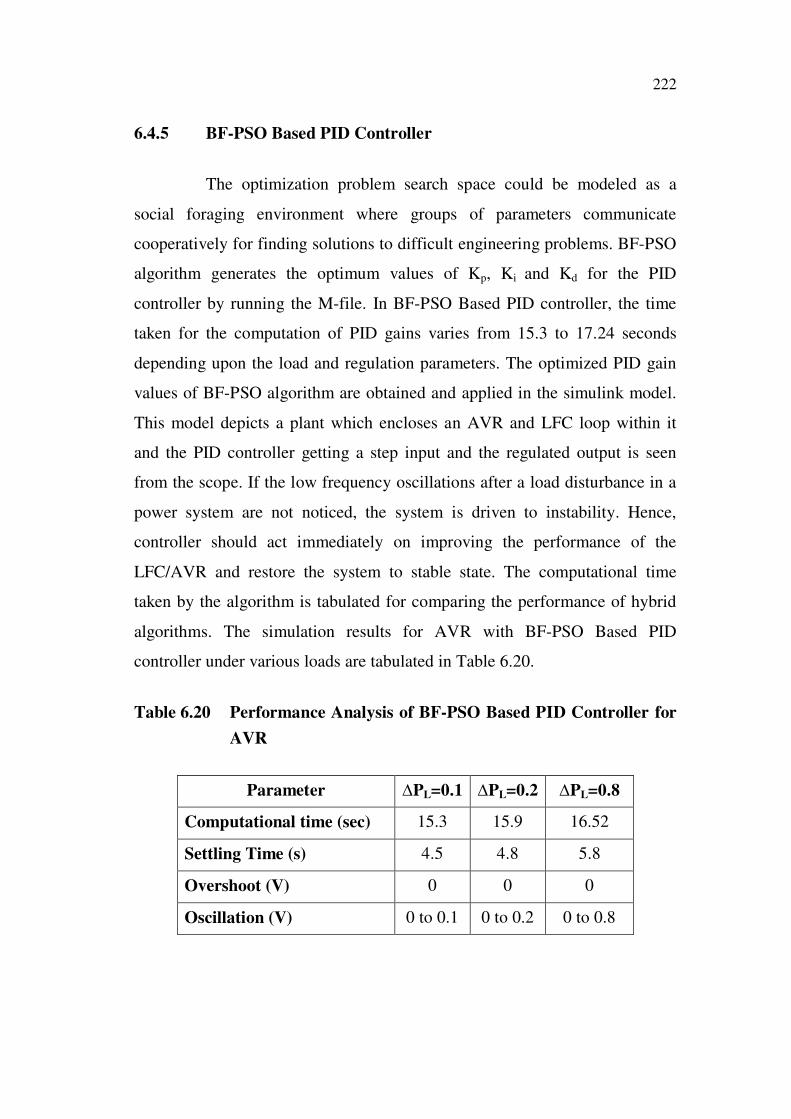
6.4.5 BF-PSO Based PID Controller

The optimization problem search space could be modeled as a

social foraging environment where groups of parameters communicate

cooperatively for finding solutions to difficult engineering problems. BF-PSO

algorithm generates the optimum values of Kp, Ki and Kd for the PID

controller by running the M-file. In BF-PSO Based PID controller, the time

taken for the computation of PID gains varies from 15.3 to 17.24 seconds

depending upon the load and regulation parameters. The optimized PID gain

values of BF-PSO algorithm are obtained and applied in the simulink model.

This model depicts a plant which encloses an AVR and LFC loop within it

and the PID controller getting a step input and the regulated output is seen

from the scope. If the low frequency oscillations after a load disturbance in a

power system are not noticed, the system is driven to instability. Hence,

controller should act immediately on improving the performance of the

LFC/AVR and restore the system to stable state. The computational time

taken by the algorithm is tabulated for comparing the performance of hybrid

algorithms. The simulation results for AVR with BF-PSO Based PID

controller under various loads are tabulated in Table 6.20.

Table 6.20 Performance Analysis of BF-PSO Based PID Controller for

AVR

Parameter PL=0.1 PL=0.2 PL=0.8

Computational time (sec) 15.3 15.9 16.52

Settling Time (s) 4.5 4.8 5.8

Overshoot (V) 0 0 0

Oscillation (V) 0 to 0.1 0 to 0.2 0 to 0.8

223

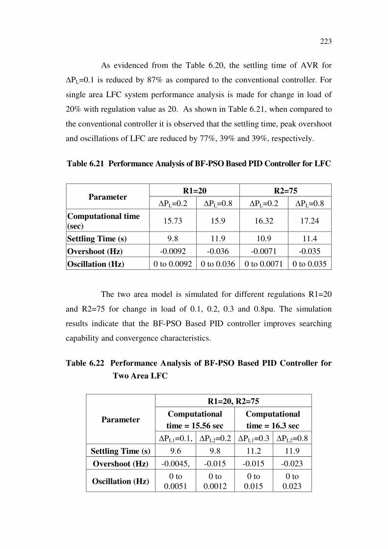
As evidenced from the Table 6.20, the settling time of AVR for

PL=0.1 is reduced by 87% as compared to the conventional controller. For

single area LFC system performance analysis is made for change in load of

20% with regulation value as 20. As shown in Table 6.21, when compared to

the conventional controller it is observed that the settling time, peak overshoot

and oscillations of LFC are reduced by 77%, 39% and 39%, respectively.

Table 6.21 Performance Analysis of BF-PSO Based PID Controller for LFC

R1=20 R2=75Parameter

PL=0.2 PL=0.8 PL=0.2 PL=0.8

Computational time

(sec)15.73 15.9 16.32 17.24

Settling Time (s) 9.8 11.9 10.9 11.4

Overshoot (Hz) -0.0092 -0.036 -0.0071 -0.035

Oscillation (Hz) 0 to 0.0092 0 to 0.036 0 to 0.0071 0 to 0.035

The two area model is simulated for different regulations R1=20

and R2=75 for change in load of 0.1, 0.2, 0.3 and 0.8pu. The simulation

results indicate that the BF-PSO Based PID controller improves searching

capability and convergence characteristics.

Table 6.22 Performance Analysis of BF-PSO Based PID Controller for

Two Area LFC

R1=20, R2=75

Computational

time = 15.56 sec

Computational

time = 16.3 secParameter

PL1=0.1, PL2=0.2 PL1=0.3 PL2=0.8

Settling Time (s) 9.6 9.8 11.2 11.9

Overshoot (Hz) -0.0045, -0.015 -0.015 -0.023

Oscillation (Hz)0 to

0.0051

0 to

0.0012

0 to

0.015

0 to

0.023

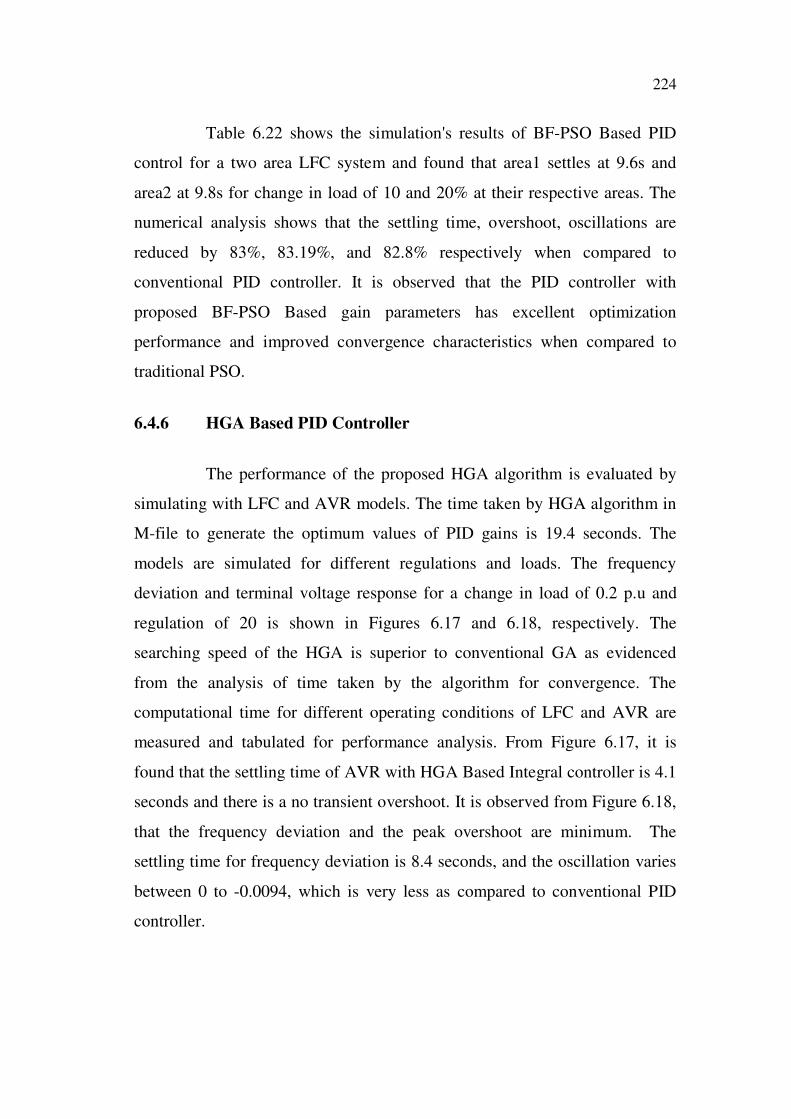
224

Table 6.22 shows the simulation's results of BF-PSO Based PID

control for a two area LFC system and found that area1 settles at 9.6s and

area2 at 9.8s for change in load of 10 and 20% at their respective areas. The

numerical analysis shows that the settling time, overshoot, oscillations are

reduced by 83%, 83.19%, and 82.8% respectively when compared to

conventional PID controller. It is observed that the PID controller with

proposed BF-PSO Based gain parameters has excellent optimization

performance and improved convergence characteristics when compared to

traditional PSO.

6.4.6 HGA Based PID Controller

The performance of the proposed HGA algorithm is evaluated by

simulating with LFC and AVR models. The time taken by HGA algorithm in

M-file to generate the optimum values of PID gains is 19.4 seconds. The

models are simulated for different regulations and loads. The frequency

deviation and terminal voltage response for a change in load of 0.2 p.u and

regulation of 20 is shown in Figures 6.17 and 6.18, respectively. The

searching speed of the HGA is superior to conventional GA as evidenced

from the analysis of time taken by the algorithm for convergence. The

computational time for different operating conditions of LFC and AVR are

measured and tabulated for performance analysis. From Figure 6.17, it is

found that the settling time of AVR with HGA Based Integral controller is 4.1

seconds and there is a no transient overshoot. It is observed from Figure 6.18,

that the frequency deviation and the peak overshoot are minimum. The

settling time for frequency deviation is 8.4 seconds, and the oscillation varies

between 0 to -0.0094, which is very less as compared to conventional PID

controller.

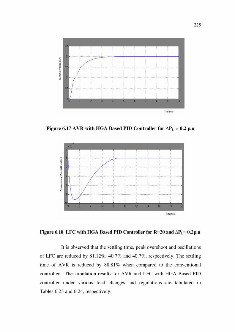
225

Figure 6.17 AVR with HGA Based PID Controller for PL = 0.2 p.u

Figure 6.18 LFC with HGA Based PID Controller for R=20 and PL= 0.2p.u

It is observed that the settling time, peak overshoot and oscillations

of LFC are reduced by 81.12%, 40.7% and 40.7%, respectively. The settling

time of AVR is reduced by 88.81% when compared to the conventional

controller. The simulation results for AVR and LFC with HGA Based PID

controller under various load changes and regulations are tabulated in

Tables 6.23 and 6.24, respectively.

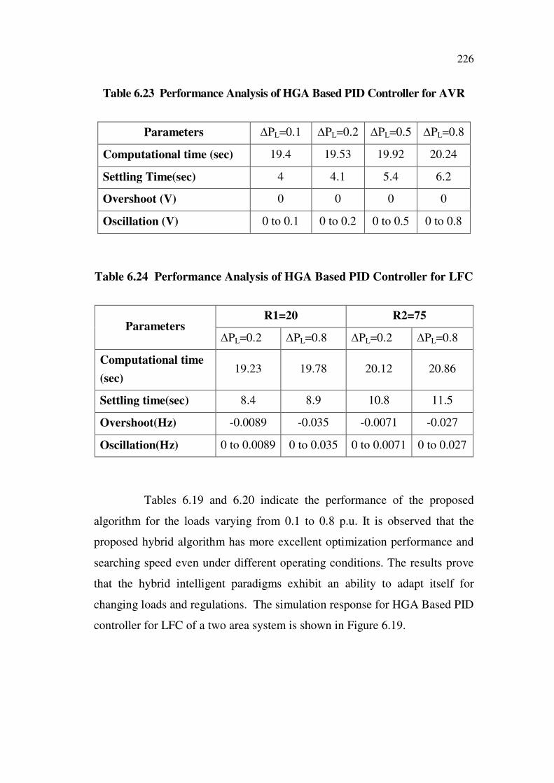
226

Table 6.23 Performance Analysis of HGA Based PID Controller for AVR

Parameters PL=0.1 PL=0.2 PL=0.5 PL=0.8

Computational time (sec) 19.4 19.53 19.92 20.24

Settling Time(sec) 4 4.1 5.4 6.2

Overshoot (V) 0 0 0 0

Oscillation (V) 0 to 0.1 0 to 0.2 0 to 0.5 0 to 0.8

Table 6.24 Performance Analysis of HGA Based PID Controller for LFC

R1=20 R2=75Parameters

PL=0.2 PL=0.8 PL=0.2 PL=0.8

Computational time

(sec)19.23 19.78 20.12 20.86

Settling time(sec) 8.4 8.9 10.8 11.5

Overshoot(Hz) -0.0089 -0.035 -0.0071 -0.027

Oscillation(Hz) 0 to 0.0089 0 to 0.035 0 to 0.0071 0 to 0.027

Tables 6.19 and 6.20 indicate the performance of the proposed

algorithm for the loads varying from 0.1 to 0.8 p.u. It is observed that the

proposed hybrid algorithm has more excellent optimization performance and

searching speed even under different operating conditions. The results prove

that the hybrid intelligent paradigms exhibit an ability to adapt itself for

changing loads and regulations. The simulation response for HGA Based PID

controller for LFC of a two area system is shown in Figure 6.19.

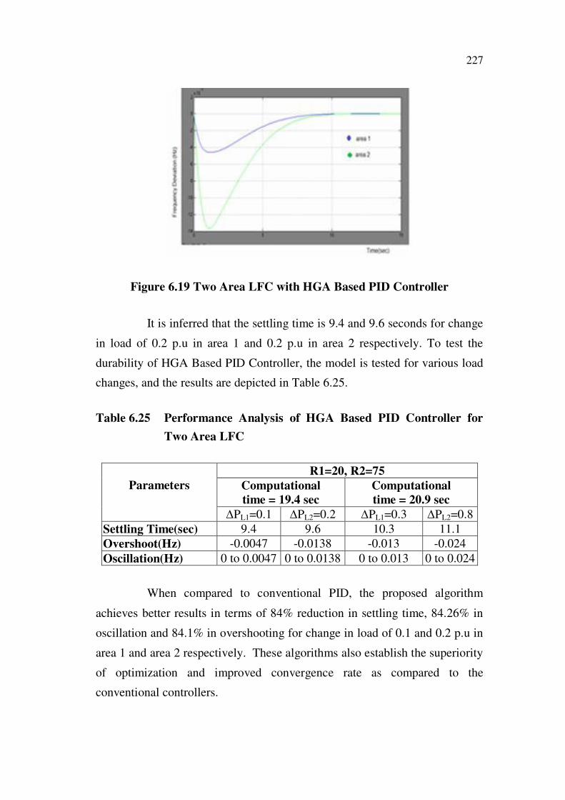
227

Figure 6.19 Two Area LFC with HGA Based PID Controller

It is inferred that the settling time is 9.4 and 9.6 seconds for change

in load of 0.2 p.u in area 1 and 0.2 p.u in area 2 respectively. To test the

durability of HGA Based PID Controller, the model is tested for various load

changes, and the results are depicted in Table 6.25.

Table 6.25 Performance Analysis of HGA Based PID Controller for

Two Area LFC

R1=20, R2=75

Computational

time = 19.4 sec

Computational

time = 20.9 sec

Parameters

PL1=0.1 PL2=0.2 PL1=0.3 PL2=0.8

Settling Time(sec) 9.4 9.6 10.3 11.1

Overshoot(Hz) -0.0047 -0.0138 -0.013 -0.024

Oscillation(Hz) 0 to 0.0047 0 to 0.0138 0 to 0.013 0 to 0.024

When compared to conventional PID, the proposed algorithm

achieves better results in terms of 84% reduction in settling time, 84.26% in

oscillation and 84.1% in overshooting for change in load of 0.1 and 0.2 p.u in

area 1 and area 2 respectively. These algorithms also establish the superiority

of optimization and improved convergence rate as compared to the

conventional controllers.

228

6.5 COMPARATIVE ANALYSIS

When an electrical load change occurs, the turbine-generator rotor

accelerates or decelerates, and frequency undergoes a transient disturbance.

The controller should not allow transient oscillations or overshoot, which in-

turn trips the under-frequency relay connected in the system. Oscillations,

settling time and overshoot are interrelated changes in reducing one parameter

will affect the other parameter. Hence, it is important that the designed

controller must be efficient in selecting the optimum gains in order to achieve

better results. Owing to the randomness of the heuristic algorithms, their

performance cannot be judged by a single result; that is to say the models are

simulated for different load changes and regulations to validate the efficiency

of the proposed algorithms (Liang Qin et al 2006). The value of R determines

the slope of the governor characteristics, and it determines the change on the

output for a given change in frequency. In practice ‘R’ is set on each generating

unit so that change in load on a system will be compensated by generated

output. The speed governor system should be operated within the restricted

control range of feedback gains due to the system instability. So, higher value

of load PL for a small ‘R’ value will introduce oscillations into the system.

Hence PL and R are selected as shown in Tables 6.23 and 6.24 to obtain

optimum results in terms of settling time, overshoot and oscillations. Increasing

the load PL into higher values will experience large overshoot and settling time.

6.5.1 Performance of Single Area System

The performance of the proposed EA Based controllers developed

for AVR of the power generating system for various load changes is given in

Table 6.26 and Table 6.27 to indicate the efficiency of PSO algorithm for

real-time applications and its suitability under varying load conditions. The

computational time required for the algorithm to compute the values of PID

gains is tabulated for performance comparison. The EA provides better

convergence and reveals their superiority with respect to settling time,

oscillations and overshoot when compared to the standard PSO method.

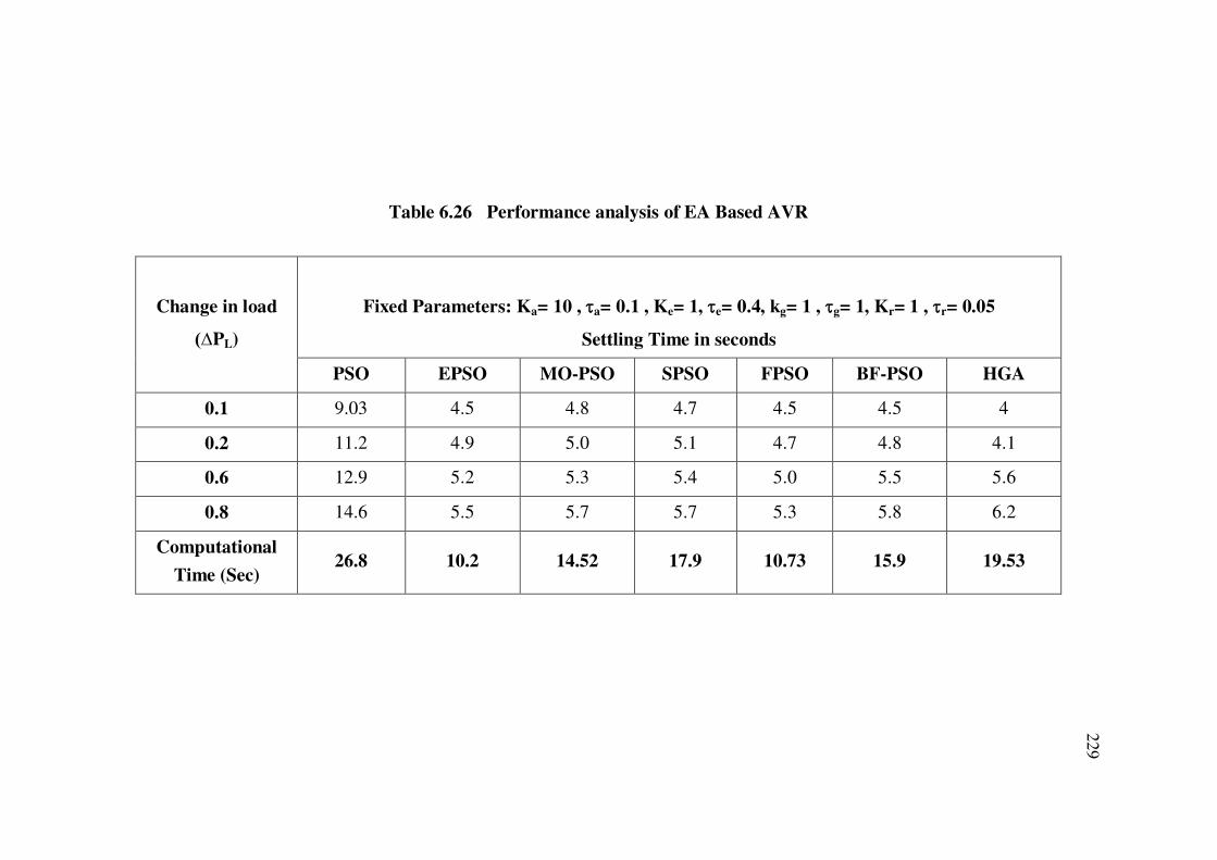
229

Table 6.26 Performance analysis of EA Based AVR

Fixed Parameters: Ka= 10 , a= 0.1 , Ke= 1, e= 0.4, kg= 1 , g= 1, Kr= 1 , r= 0.05

Settling Time in seconds

Change in load

PL)

PSO EPSO MO-PSO SPSO FPSO BF-PSO HGA

0.1 9.03 4.5 4.8 4.7 4.5 4.5 4

0.2 11.2 4.9 5.0 5.1 4.7 4.8 4.1

0.6 12.9 5.2 5.3 5.4 5.0 5.5 5.6

0.8 14.6 5.5 5.7 5.7 5.3 5.8 6.2

Computational

Time (Sec)26.8 10.2 14.52 17.9 10.73 15.9 19.53

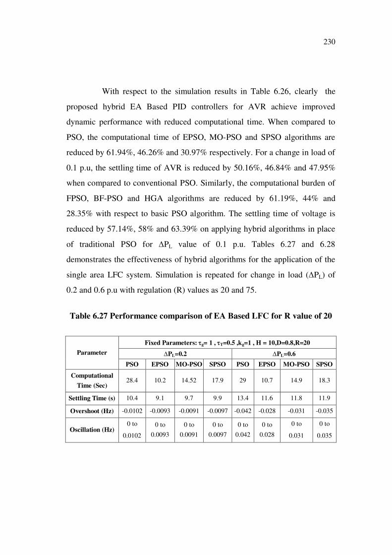
230

With respect to the simulation results in Table 6.26, clearly the

proposed hybrid EA Based PID controllers for AVR achieve improved

dynamic performance with reduced computational time. When compared to

PSO, the computational time of EPSO, MO-PSO and SPSO algorithms are

reduced by 61.94%, 46.26% and 30.97% respectively. For a change in load of

0.1 p.u, the settling time of AVR is reduced by 50.16%, 46.84% and 47.95%

when compared to conventional PSO. Similarly, the computational burden of

FPSO, BF-PSO and HGA algorithms are reduced by 61.19%, 44% and

28.35% with respect to basic PSO algorithm. The settling time of voltage is

reduced by 57.14%, 58% and 63.39% on applying hybrid algorithms in place

of traditional PSO for PL value of 0.1 p.u. Tables 6.27 and 6.28

demonstrates the effectiveness of hybrid algorithms for the application of the

single area LFC system. Simulation is repeated for change in load ( PL) of

0.2 and 0.6 p.u with regulation (R) values as 20 and 75.

Table 6.27 Performance comparison of EA Based LFC for R value of 20

Fixed Parameters: g= 1 , T=0.5 ,kg=1 , H = 10,D=0.8,R=20

PL=0.2 PL=0.6Parameter

PSO EPSO MO-PSO SPSO PSO EPSO MO-PSO SPSO

Computational

Time (Sec)28.4 10.2 14.52 17.9 29 10.7 14.9 18.3

Settling Time (s) 10.4 9.1 9.7 9.9 13.4 11.6 11.8 11.9

Overshoot (Hz) -0.0102 -0.0093 -0.0091 -0.0097 -0.042 -0.028 -0.031 -0.035

Oscillation (Hz)0 to

0.0102

0 to

0.0093

0 to

0.0091

0 to

0.0097

0 to

0.042

0 to

0.028

0 to

0.031

0 to

0.035

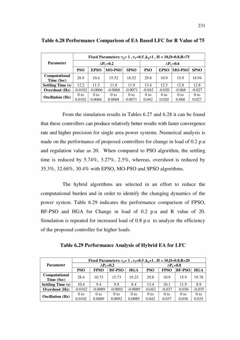
231

Table 6.28 Performance Comparison of EA Based LFC for R Value of 75

Fixed Parameters: g= 1 , T=0.5 ,kg=1 , H = 10,D=0.8,R=75

PL=0.2 PL=0.6Parameter

PSO EPSO MO-PSO SPSO PSO EPSO MO-PSO SPSO

Computational

Time (Sec)28.9 10.4 15.52 18.52 29.8 10.9 15.9 18.94

Settling Time (s) 12.2 11.5 11.8 11.9 13.4 12.5 12.8 12.8

Overshoot (Hz) -0.0102 -0.0066 -0.0068 -0.0071 -0.042 -0.020 -0.068 -0.027

Oscillation (Hz)0 to

0.0102

0 to

0.0066

0 to

0.0068

0 to

0.0071

0 to

0.042

0 to

0.020

0 to

0.068

0 to

0.027

From the simulation results in Tables 6.27 and 6.28 it can be found

that these controllers can produce relatively better results with faster convergence

rate and higher precision for single area power systems. Numerical analysis is

made on the performance of proposed controllers for change in load of 0.2 p.u

and regulation value as 20. When compared to PSO algorithm, the settling

time is reduced by 5.74%, 3.27%, 2.5%, whereas, overshoot is reduced by

35.3%, 32.68%, 30.4% with EPSO, MO-PSO and SPSO algorithms.

The hybrid algorithms are selected in an effort to reduce the

computational burden and in order to identify the changing dynamics of the

power system. Table 6.29 indicates the performance comparison of FPSO,

BF-PSO and HGA for Change in load of 0.2 p.u and R value of 20.

Simulation is repeated for increased load of 0.8 p.u to analyze the efficiency

of the proposed controller for higher loads.

Table 6.29 Performance Analysis of Hybrid EA for LFC

Fixed Parameters: g= 1 , T=0.5 ,kg=1 , H = 10,D=0.8,R=20

PL=0.2 PL=0.8Parameter

PSO FPSO BF-PSO HGA PSO FPSO BF-PSO HGA

Computational

Time (Sec)28.4 10.73 15.73 19.23 29.8 10.9 15.9 19.78

Settling Time (s) 10.4 9.4 9.8 8.4 13.4 10.1 11.9 8.9

Overshoot (Hz) -0.0102 -0.0089 -0.0092 -0.0089 -0.042 -0.037 -0.036 -0.035

Oscillation (Hz)0 to

0.0102

0 to

0.0089

0 to

0.0092

0 to

0.0089

0 to

0.042

0 to

0.037

0 to

0.036

0 to

0.035

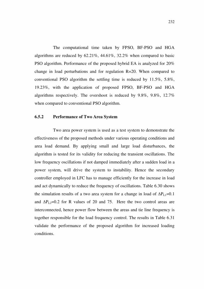
232

The computational time taken by FPSO, BF-PSO and HGA

algorithms are reduced by 62.21%, 44.61%, 32.2% when compared to basic

PSO algorithm. Performance of the proposed hybrid EA is analyzed for 20%

change in load perturbations and for regulation R=20. When compared to

conventional PSO algorithm the settling time is reduced by 11.5%, 5.8%,

19.23%, with the application of proposed FPSO, BF-PSO and HGA

algorithms respectively. The overshoot is reduced by 9.8%, 9.8%, 12.7%

when compared to conventional PSO algorithm.

6.5.2 Performance of Two Area System

Two area power system is used as a test system to demonstrate the

effectiveness of the proposed methods under various operating conditions and

area load demand. By applying small and large load disturbances, the

algorithm is tested for its validity for reducing the transient oscillations. The

low frequency oscillations if not damped immediately after a sudden load in a

power system, will drive the system to instability. Hence the secondary

controller employed in LFC has to manage efficiently for the increase in load

and act dynamically to reduce the frequency of oscillations. Table 6.30 shows

the simulation results of a two area system for a change in load of PL1=0.1

and PL2=0.2 for R values of 20 and 75. Here the two control areas are

interconnected, hence power flow between the areas and tie line frequency is

together responsible for the load frequency control. The results in Table 6.31

validate the performance of the proposed algorithm for increased loading

conditions.

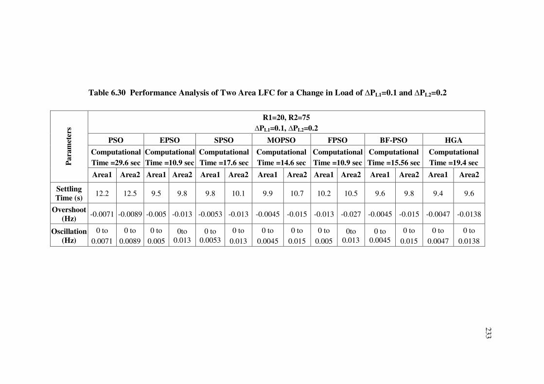
233

Table 6.30 Performance Analysis of Two Area LFC for a Change in Load of PL1=0.1 and PL2=0.2

R1=20, R2=75

PL1=0.1, PL2=0.2

PSO EPSO SPSO MOPSO FPSO BF-PSO HGA

Computational

Time =29.6 sec

Computational

Time =10.9 sec

Computational

Time =17.6 sec

Computational

Time =14.6 sec

Computational

Time =10.9 sec

Computational

Time =15.56 sec

Computational

Time =19.4 secPa

ram

eter

s

Area1 Area2 Area1 Area2 Area1 Area2 Area1 Area2 Area1 Area2 Area1 Area2 Area1 Area2

Settling

Time (s)12.2 12.5 9.5 9.8 9.8 10.1 9.9 10.7 10.2 10.5 9.6 9.8 9.4 9.6

Overshoot

(Hz)-0.0071 -0.0089 -0.005 -0.013 -0.0053 -0.013 -0.0045 -0.015 -0.013 -0.027 -0.0045 -0.015 -0.0047 -0.0138

Oscillation

(Hz)

0 to

0.0071

0 to

0.0089

0 to

0.005

0to

0.013

0 to

0.0053

0 to

0.013

0 to

0.0045

0 to

0.015

0 to

0.005

0to

0.013

0 to

0.0045

0 to

0.015

0 to

0.0047

0 to

0.0138

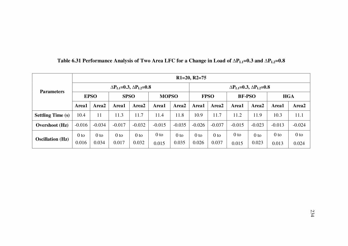
234

Table 6.31 Performance Analysis of Two Area LFC for a Change in Load of PL1=0.3 and PL2=0.8

R1=20, R2=75

PL1=0.3, PL2=0.8 PL1=0.3, PL2=0.8

EPSO SPSO MOPSO FPSO BF-PSO HGAParameters

Area1 Area2 Area1 Area2 Area1 Area2 Area1 Area2 Area1 Area2 Area1 Area2

Settling Time (s) 10.4 11 11.3 11.7 11.4 11.8 10.9 11.7 11.2 11.9 10.3 11.1

Overshoot (Hz) -0.016 -0.034 -0.017 -0.032 -0.015 -0.035 -0.026 -0.037 -0.015 -0.023 -0.013 -0.024

Oscillation (Hz)0 to

0.016

0 to

0.034

0 to

0.017

0 to

0.032

0 to

0.015

0 to

0.035

0 to

0.026

0 to

0.037

0 to

0.015

0 to

0.023

0 to

0.013

0 to

0.024

235

From the simulation results, it reveals that the hybrid EA method is

a potential alternative to be implemented as a useful tool in solving power

quality problems. As shown in Table 6.30, the settling time is reduced by

21%, 13.28%, 13.3%, 14.84%, 12.5%, 19.50% with application of EPSO,

SPSO, MO-PSO, FPSO, BF-PSO, and HGA algorithms respectively. In terms

of overshoot and oscillations the proposed hybrid algorithms attain reduction

of 15.15%, 18.2%, 12.13%, 21.2%, 30% and 27.3% in comparison with PSO

algorithm. The investigation is carried out for increased load of 0.3p.u in

area1 and 0.8p.u in area2 and the results in Table 6.31 explore the possibilities

of proposed algorithms for different operating conditions. When a change in

load is small, the overshoot and the settling time in the response is reduced.

Therefore, we can choose appropriate gains Based on estimation to overshoot,

oscillations and settling time.

6.6 COMPUTATIONAL EFFICIENCY OF EVOLUTIONARY

ALGORITHMS

The trend in present research and development of PID controller is

to focus on the fast and reliable methods in order obtain the best performance

of existing PID control. Hence intelligent optimization techniques are

developed to decrease the computational time with increased reliability and

efficiency of the controller. The inclusion of hybrid evolutionary algorithms

in PID gain tuning helps to automate the entire design process to a useful

degree. The comparison of average computation time or time complexity of

different hybrid EAs for combinatorial optimization of PID gains for AVR

and LFC is shown in Figure 6.20.

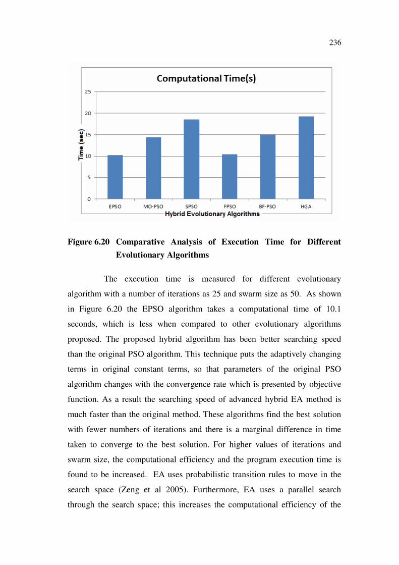
236

Figure 6.20 Comparative Analysis of Execution Time for Different

Evolutionary Algorithms

The execution time is measured for different evolutionary

algorithm with a number of iterations as 25 and swarm size as 50. As shown

in Figure 6.20 the EPSO algorithm takes a computational time of 10.1

seconds, which is less when compared to other evolutionary algorithms

proposed. The proposed hybrid algorithm has been better searching speed

than the original PSO algorithm. This technique puts the adaptively changing

terms in original constant terms, so that parameters of the original PSO

algorithm changes with the convergence rate which is presented by objective

function. As a result the searching speed of advanced hybrid EA method is

much faster than the original method. These algorithms find the best solution

with fewer numbers of iterations and there is a marginal difference in time

taken to converge to the best solution. For higher values of iterations and

swarm size, the computational efficiency and the program execution time is

found to be increased. EA uses probabilistic transition rules to move in the

search space (Zeng et al 2005). Furthermore, EA uses a parallel search

through the search space; this increases the computational efficiency of the

237

algorithms. The no-free-lunch (NFL) theorem states that there cannot exist

any algorithm for solving all problems that are on average superior to any

other algorithm. This theorem motivates research in new optimization

algorithms, especially EA. Since, the basic PSO method does not perform the

selection and crossover operation in the evolutionary process, it can save

computation time compared with the GA method, thus proving that the EA

Based PID controller is more superior. The EA search starts from a diverse set

of initial points, which allows parallel search of a large area of the search

space.

6.7 SUMMARY

A novel hybrid EA is designed for determining the PID controller

parameters for LFC and AVR of the power generating system. The hybrid

algorithms generate better solutions by improving the global and local search

ability of the PSO and overcome the disadvantages of the PSO. In order to

identify the changing dynamics of the power system and to provide necessary

control actions, high computational power is needed. These algorithms are

selected in an effort to reduce the computational burden and to improve the

computational efficiency of PSO.

The LFC and AVR models with EPSO, MO-PSO, SPSO, HGA,

BF-PSO, and FPSO Based controllers are simulated for different operating

conditions for performance comparison. The experimental results indicate that

the proposed hybrid EA Based controllers can improve the computational

efficiency and produce more satisfactory output. Compared to conventional

fixed gain controllers, the suggested algorithms perform well under all

regions of operations with increased performance characteristics.

The proposed algorithm has the potential stability in overcoming

the possibility of entrapment in local minimum solutions. Hence, the

238

application of hybrid algorithms improves the dynamic response of voltage

and frequency responses of the autonomous and interconnected power

generating system. The combined and synergic use of information yields a

promising tool in solving power system control problems that require

optimization of more parameters. From the simulation results of two areas

interconnected system, it reveals that these controllers can generate good

quality solutions at higher precision.

In future, the work can be extended by simulating the algorithm for

different types of turbine models and with different system parameters. The

applications of hybrid EA Based controllers can be extended for multi-area

power system, including non-linear parameters. The intelligent hybrid

techniques like, GA-SA, Neuro-fuzzy-GA, Neuro-fuzzy-PSO, Neuro-fuzzy-

ACO can be implemented to enhance the performance of the generating

system.