Embed Size (px)
Citation preview

Chapter 6
M I C R O S C O P I C B A L A N C E S
In this chapter, we develop microscopic balances that are used for the simulation of distributed parameter systems. Distributed systems have spatial gradients as well as time changes. In order to properly describe these systems, the conservation laws must be applied to any point within the system rather than written over the entire macroscopic system. Not only will these point or microscopic conservation laws be developed in this chapter, but they will also be applied to several classical one- dimensional problems that have either analytical solutions or are initial- value problems that can be solved using computational techniques al- ready introduced and discussed. An excellent treatment of microscopic balances is found in the book by Bird, Stewart, and Lightfoot (1960). Simplification of complex problems using order-of-magnitude analysis is also introduced.
6.1 CONSERVATION OF TOTAL MASS (EQUATION OF CONTINUITY)
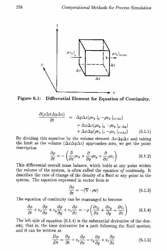
The equation of continuity is derived by writing a mass balance over an arbitrary finite volume element AxAyAz through which a fluid is flowing, as is shown in Figure 6.1. We then take the limit as the volume element goes to zero to get the appropriate equation for any point in the spatial domain.
The rate of mass entering the volume element perpendicular to the x axis at x is pv~AyAz I~ and at the plane x + Ax is pv~AyAz i~+~ Similar expressions can be written for the other planes. The rate of accumulation of mass within the volume element is O(pAxAyAz)/Ot. The mass balance therefore becomes
Rate of Rate of Rate of Accumulation of Mass Mass In Mass Out
258 Computational Methods for Process Simulation
Figure 6.1"
P V x [ X
i |
~y \
2~x
• ~ x
Differential Element for Equation of Continuity.
O(pAzAyAz) ot
+ xAz(pv I -pv + Ax y( z Iz-pVz (6.1.1)
By dividing this equation by the volume element AxAyAz and taking the limit as the volume (AxAyAz) approaches zero, we get the point description
O----t = - pv~ + ~y pVy + -~z pVz (6.1.2)
This differential overall mass balance, which holds at any point within the volume of the system, is often called the equation of continuity. It describes the rate of change of the density of a fluid at any point in the system. The equation expressed in vector form is
Op 0--t = - ( V - p v ) (6.1.3)
The equation of continuity can be rearranged to become
Op Op Op Op ( Ov~ Ovy Ovz ) 0--7 + Vx~xx + Vy~y + v ~ z - - p ~ x + N + ~ (6.1.4)
The left side of equation (6.1.4) is the substantial derivative of the den- sity, that is, the time derivative for a path following the fluid motion; and it can be written as
D p _ Op Op Op Op (6.1.5) D t - O--t + v~-~x + v y-~y + v~ Oz

Microscopic Balances 259
A very important special form of the equation of continuity is that for a fluid of constant density (incompressible fluid), for which the substantial derivative is zero. Equation (6.1.4) therefore becomes for an incompress- ible fluid,
V . v = 0 (6.1.6)
6.2 C O N S E R V A T I O N OF C O M P O N E N T i
The mass balance for a species component i in a multicomponent mixture must also consider the rate of generation of the component by chemical reaction. The mass conservation law becomes
Rate of Rate In of
Accumulation = Component i of Component i
Rate Out of Component i
Rate of + Generation of
Component i
OpiAxAyAz ot - ~ y ~ X z ( p ~ I~-p~ I~+~)
+ ~~z(p~vi~ I~ - p ~ I~÷~) + ~x~y(p~V~z I~ -p~.z Ez÷~z) + ri(AxAyAz) (6.2.1)
where ri is the rate of generation of i per unit volume. By dividing this equation by the volume elementAxAyAz and taking
the limit as these dimensions go to zero, we have
Op~ _ ( O 0 O ) Ot -- -- -~X pivix + -~ypiViy + -~zpiViz + ri (6.2.2)
Recognizing that pivi~ is the mass flux of i in the x direction, ni~, we can write equation (6.2.2) as
Opi _ _ ( i)nix Oniy Onix ) Ot - \ Ox + -~y + Oz + ri (6.2.3)
In vector notation we have
Opi Ot = - ( V . hi)+ ri (6.2.4)
For systems in which molecular diffusion occurs, the mass flux is the sum of the bulk flow of species i and the diffusional flux of that species.
N
j -1 (6.2.5)

260 Computational Methods for Process Simulation
where v = the mass average velocity of the fluid w~- mass fraction N = number of components J i - the diffusional flux
For binary diffusion we can relate the diffusional flux to the concentration gradient via Fick's first law.
J A -- --[9"DAB V W A (6.2.6)
where ~ A B = the binary diffusion coefficient (.d A - - the mass fraction of A
To obtain the component bala~nces in molar units, it is only necessary to divide the mass expressions by the molecular weight of the specific component:
Molar concentration = Ci = pi/Mi Molar flux = Ni = ni/Mi Molar rate of generation per unit volume = Ri -- ri /Mi
Therefore the component balance equation, (6.2.4), becomes
0-T + V. N ~ - Ri (6.2.7)
In terms of the bulk flow and diffusional flux we have
N
N i - Civ* + J~ - xi ~ N j + J~ , xi - mole fraction (6.2.8) j - - 1
where v* is the molar average velocity and for binary systems the molar flux J~4 is given by Fick's law to be
J*A - - - C ~ A B V X A (6.2.9)
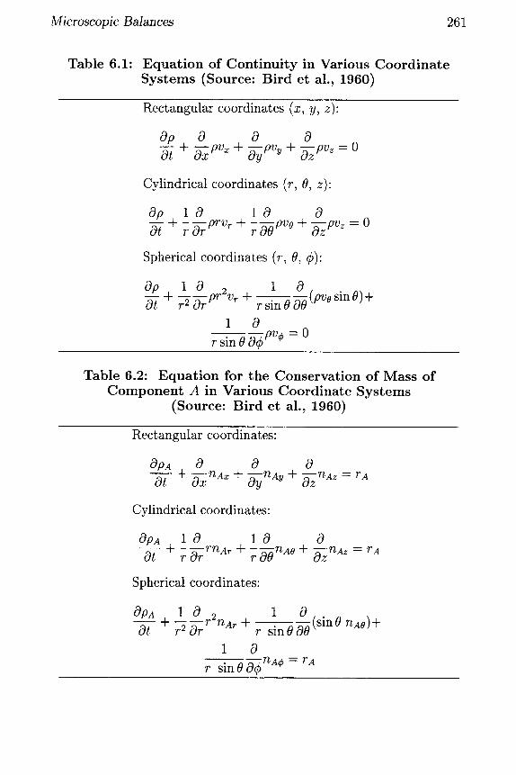
Here X A is the mole fraction of A. A summary of the various component and overall mass balances is
found in Tables 6.1, 6.2, and 6.3.
6.3 D I S P E R S I O N D E S C R I P T I O N
For mass transport problems that do not involve molecular diffusion, such as turbulent-flow problems, or problems with highly complicated passages such as packed beds or porous media, a dispersion model is usually used. Here we assume that the controlling mass transport mech- anisms are similar in character to the molecular case; and, therefore,
Microscopic Balances 261
Table 6.1" Equation of Continuity in Various Coordinate Systems (Source: Bird et al., 1960)
Rectangular coordinates (x, y, z):
Op 0 0 0 0--7 + -~x pvz + -~y pVy ÷ -~zpVz - 0
Cylindrical coordinates (r, 0, z):
0p 1 0 1 0 0 O---t -t- -r -~r pr v r + -r - ~ PV e + -~z pV z - 0
Spherical coordinates (r, 0, ¢):
Op 1 0 + -==-pr2v
o-7 rz ur
1 0 r sin 0 00 (pvo sin 0)+
1 0 r sin 0 0¢ pv¢ - 0
Table 6.2" Equation for the Conservation of Mass of Component A in Various Coordinate Systems
(Source: Bird et al., 1960)
Rectangular coordinates:
OpA 0 0 0 Ot !- --~x?~Ax ~ ~ ~ -- ?~A - Oy?~Ay -~zT~Az
Cylindrical coordinates:
OpA
Ot
1 0 1 0 0 -~- - r ÷ - -t- -~z n Az -- r A r-~r na t r - ~ n A °
Spherical coordinates:
~PA 1 0 r2 0-7 + +
1 ~0 (sin 0 nAO)+ r sin ~ 00
1 0 r sin ~ 0---¢ nAck rA
262 Computational Methods for Process Simulation
Table 6.3: Equa t ion of Con t inu i ty of A in a Di lu te Binary Sys tem for Cons t an t p and ~AB
(Source" Bird et al., 1960)
Rectangular coordinates:
op~ ( op~ op~ o p ~ _ o-7- + ~ ~ x + v~-~v + V z Oz ]
(02pA O2pA O2pA) AB C~X2 -+- "Oy 2 + ~ --~ 7"d
Cylindrical coordinates:
OpA ( OpA IOpA OpA~ o--i- + v~-~r + v o-r--~- + Vz Oz ] -
Z)AB -~r r ~ -~ r2 002 t- Oz 2 + r A
Spherical coordinates:
OpA ( OpA I OpA ] OpA ) O--T- + v ~ --~-r + v o - + v ¢ ~ - r ~ r sin 0 0¢
Z)AB ~ ~ r ~ -~r ] +r 2 sinO00 sinO O0 + 1 02pA ]
r2 sin2 0 0¢ 2 + r a
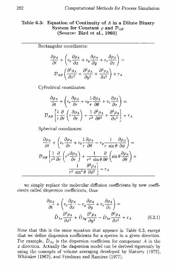
we simply replace the molecular diffusion coefficients by new coeffi- cients called dispersion coefficients, thus"
o--i- + v~-~x + ~-~y + Vz Oz ] JE) 4x 02 PA 02 PA 02 PA
Ox 2 + bA~ Oy 2 + DAz Oz 2 + rA (6.3.1)
Note that this is the same equation that appears in Table 6.3, except that we define dispersion coefficients for a species in a given direction. For example, DAx is the dispersion coefficient for component A in the x direction. Actually the dispersion model can be derived rigorously by using the concepts of volume averaging developed by Slattery (1972), Whitaker (1962), and Friedman and Ramirez (1977).

Microscopic Balances 263
6.4 M E T H O D OF W O R K I N G P R O B L E M S
There are basically two attacks to setting up microscopic balance prob- lems. These are to define the differential volume element for the problem at hand and then derive the describing equation, or to simplify the gen- eral equations. For problems with simple geometries, it is best to develop the equations for the individual case under study as the first step. In order to check the development, the general equations can then be sim- plified to make sure that the same describing equation set results. For problems with complicated geometries, it is probably best first to sim- plify the general equations.
6.5 S T A G N A N T F I L M D I F F U S I O N
Let us consider the problem of determining the steady-state rate of evap- oration into a stagnant nonmoving volume of gas over an open liquid surface, as shown in Figure6.2.
Free flowing gas B, xnt
z = L AZ
Stagnant Gas B
z-ol_. - 1 Liquid A
Figure 6.2" Stagnant Film Diffusion.
The mole fraction of vapor A in the free-flowing gas (z = L) is X AL, while that at the vapor-liquid surface (z = 0) is xAO. The vapor concen- tration at z = 0 can be computed from knowledge of the vapor pressure of liquid A. In order to solve this problem, we write a component material balance over a differential volume element S A z . A differential element in only one dimension (Az) is needed because the concentration is only a function of the one dimension, z.
Rate of Rate In Accumulation =
of ComponentA of Component A
Rate Out of Component A
O-- NAS Iz --NA lz+az (6.5.1)
264 Computa t ional Methods for Process Simulation
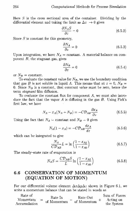
Here S is the cross-sectional area of the container. Dividing by the differential element and taking the limit as Az --+ 0 gives
ONAS = o (6 .5 .2)
Oz
Since S is constant for this geometry,
ONA = o (6 .5 .3)
Oz
Upon integration, we have NA -- constant. A material balance on com- ponent B, the stagnant gas, gives
ONB = 0 (6.5.4)
Oz
or NB -- constant. To evaluate the constant value for NB, we use the boundary condition
that gas B is not soluble in liquid A. This means that at z - 0, NB -- 0. Since NB is a constant, that constant value must be zero, hence the term s tagnant film diffusion.
To evaluate the constant flux for component A, we must also intro- duce the fact that the vapor A is diffusing in the gas B. Using Fick's first law, we have
NA -- XA(NA + NB) -- --C:DAB OxA (6.5.5) OZ
Using the fact that NA -- constant and NB -- 0 gives
dxn NA(1 -- Xn) -- --C:DAB d---~- (6.5.6)
which can be integrated to give
NA L - I n (1--XAL ) (6.5.7) CT)AB 1 -- XAO
The steady-state rate of evaporation is
N A S = C ~ A B S ln ( I -- XAL) (6.5.8) L 1 - xAO
6.6 CONSERVATION OF MOMENTUM (EQUATION OF MOTION)
For our differential volume element A x A y A z shown in Figure 6.1, we write a momentum balance that can be stated in words as
Rate of Sum of Forces Rate In Rate Out
Momentum = of Momentum - of Momentum + Acting on Accumulation the System

Microscopic Balances 265
The generation term is stated in terms of forces acting on the system. This is a consequence of Newton's second law, which states that the rate of change of momentum is equal to a force, that is, f = d(mv)/dt. It is important to realize that the momentum balance is a vector equation with components in each of three mutually orthogonal coordinate direc- tions. We will consider in this derivation only the x component of the equation of motion in rectangular coordinates.
Momentum flows into and out of the volume element by two mecha- nisms: by convection (due to the bulk flow of the fluid) and by molecular transfer (due to the velocity gradients in the system).
Let us first consider the convective mechanism for the transport of the x component of momentum (pv~). This component can enter at plane x due to the flow v~ and leave at plane x + Ax due also to the flow v~. The x component of momentum can enter the volume element at plane y due to the flow vu and exits due to this flow at plane y + Ay. The net convective x component of momentum is therefore
÷AxzXy(p v Iz-pV z Iz+ z) Now let's consider the molecular transport of momentum. The molecular mechanism is given by the stress tensor or molecular momentum flux tensor, I". Each element Tij c a n be interpreted as the jth component of momentum flux transfer in the i th direction. We are therefore interested in the terms 7~. The rate at which the x component of momentum enters the volume element at face x is z-~AyAx I~, the rate at which it leaves at face x + Ax is "r~AyAx I~+~, and the rate at which it enters at face y is Ty~AxAz ly. The net molecular contribution is therefore
In most cases the only important forces acting on the system are those arising from the fluid pressure p and the gravitational force per unit mass g. The resultant force terms are therefore
The rate of accumulation of the x component of momentum is (AxAyAx) (Opv~/Ot).
Substituting these expressions into the conservation principle, divid- ing the resulting equation by volume element AxAyAz, and taking the limit as Ax, Ay, and Az approach zero gives
0
O- pv = 0 0 0 )
- + pv vy +
- + + - + (6.6.1)

266 Computational Methods for Process Simulation
The entire vector momentum balance equation is
0 O--~pv - - I V - p v v ] - V p - [V-"r] + P9 (6.6.2)
which can give
be rearranged, with the help of the equation of continuity, to
D v = - V p - IV. 7-] + Pg (6.6.3)
Dt
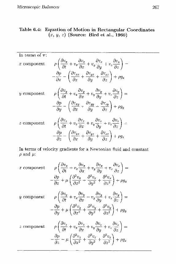
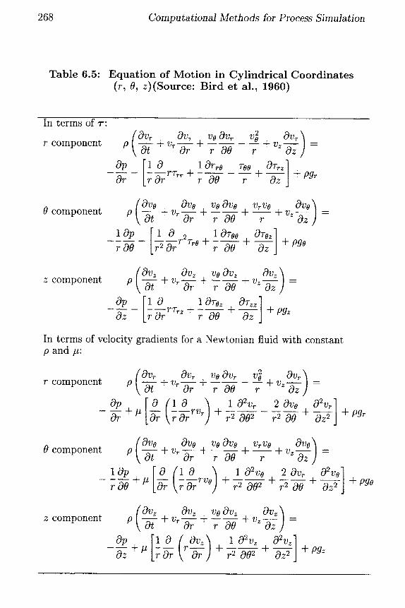
Tables 6.4, 6.5, and 6.6 show the equation of motion in several coordinate systems in terms of 7" and in terms of velocity" gradients for a Newtonian fluid.
6.7 D I S P E R S I O N D E S C R I P T I O N
For systems to be described with dispersion coefficients, we will assume that the dispersive transfer mechanisn is similar to that of the diffusion mechanism. We do not assume that all the dispersion coefficients are equal so that we have terms such as
d?)x z-y~--ftv~ dy (6.7.1)
_ dvx T ~ - - - P z ~ dz (6.7.2)
The equations for dispersion look just like those for a Newtonian fluid except we substitute the dispersion coefficients for the viscosity.
6.8 P I P E F L O W OF A N E W T O N I A N F L U I D
Here, we will apply the momentum balance to determine the steady- state radial velocity profile for the flow in a pipe of a Newtonian fluid. Figure 6.3 describes the system.
Writing a momentum balance over the incremental volume 2~rArL gives the following:
Rate of Accumulation of Component z of Momentum
Rate In = of Component z
of Momentum
Rate Out of Component z of Momentum
+ Sum of
Forces in the z Direction
©
©
m m
I + + + %
+
+ + + II
©
©
m
I + ~
1~
]::
: ~
~ +
~1 ~
~
+ + ~1
~ +d
o
+
+ ~1
~
©
©
m
I + ]::: +
+ ~q
+ +
~ + + ~17
• .
~ 0 m
©
~,,
~o
~ I ~
~
+ ~
~1 ~
~
~I ~
+ ~
+
~1 ~
~-
~
~ 0 +
= +
~
©
©
0 e,-e-
I "m
~ +
+ ~
1~
+ ~ ~
l~
~ +
+ ~1
~ II
c~
© ©
m m
e-e
I m
~ + +
+ ~
1 ~
+ ~
f~
II
°o
F~
,J
kill
0
t~
e~
• o
0 (~
0
0
m.
el'-
.m
~°
c~
b~
-.,I
268 Computational Methods for Process Simulation
Table 6.5: Equation of Motion in Cylindrical Coordinates (r, 0, z)(Source: Bird et al., 1960)
In terms of ~-:
r component ( Ov~ Ov~ vo Ov~ v~ Ova)
P _ _ _. --~+v~--~-r + . . . . r (90 r 4 - V z ~ -
Op [ ~ 0 lOrro 7-oo O~-rz] Or -~r r 7rr -~ ~- + Pgr r 00 r Oz
0 component Ovo Ovo vo Ovo v~vo Ovo ) P - ~ + v ~ - - ~ r 4 -r -~ t- r= + % ~ z -
l o p [1 0r2 107oo 07Oz] r O0 Oz Pgo
z component ( Ovz OVz vo OVz OVz ) P\ ot + ~ r T r ~ r ~ - ~ Z - ~ z -
OzCOP [10r ro l OToz OWzz ] _~. r Vr z -~ F + P gz r 00 Oz
In terms of velocity gradients for a Newtonian fluid with constant p and #:
r component
Op Or
( Ov~ OVr Vo OV~ V~ OVa) P -5~+~-g-/~ ~ oo -~ ~Vz-gTz -
+ ~ -~r -~rrv~ -t r2 002 r 2 O0 ~- Oz 2 ] + pg~
0 component Ove Ovo vo Ovo VrVO OVo p - ~ - + V r - g / ~ ~ 00 ~ .... ~ +v~-57) -
r O0 + # -~r -~r rv° -~ r 2 002 ~ r 2 O0 F OZ 2 + Pgo
z component vo vz vz) P -~-Vr'~T'~ r O0 F v~-~z - -
l O vz 1 - O z + ~ ~ r or ] -~ r 2002 ~- Oz 2 + pg~

Microscopic Balances 269
Table 6.6" E q u a t i o n of M o t i o n in Spher ica l C o o r d i n a t e s (r, 0, ¢) (Source: Bi rd et al., 1960)
In terms of r :
r component
P\ ot + V r - ~ ~ + - - r 00 r sin 6 0¢ r
Op [ 1 0 1 0 -~rr2rr~ -~ (fro sin 0) [ Or r sin 0 00
1 Or~¢ roe + r~¢~ ] + Pgr r sin 0 0 ¢ r
0 component
Ove Ove p -~+~-g7 ~
r O0 lop
ve Ore r O0
1 0
07o¢ fro r sin 0 0¢
v¢ 0% VrVe v~ cot 0) r sin 0 0¢ ~ r r
1 0 r sin 0 O0 (7oo sin 0)
cot 0 ] r r¢¢ + Pgo
¢ component
Ov¢ Ovo vo 0% P \ Ot + v~--&r ~ r O0
1 op r sin 0 0¢
+
v¢ Ov¢ VCVr vov¢ I F + cot 0 ----
r sin 0 0¢ r r ] 1 0 10tee 1 0r¢¢ -~~(~~) ~
r 00 r sin0 0¢
2cot0 ] rr¢ + ro~ + pg~ r r

270 Computational Methods for Process Simulation
Table 6.6 (cont inued)" E q u a t i o n of M o t i o n in Spher ica l C o o r d i n a t e s (r, 0, ¢) (Source" B i rd et al., 1960)
In terms of velocity gradients for a Newtonian fluid with contstant p and # "~
r component
(Ov~ Ovr P \ ot +v~-~r~
vo Ov~ v¢ Ov~ I
r 00 r sin 0 0¢
Op ( 2 20vo 2 -0---~ + ~ V2Vr - - r2 v~ r 2 O0 r2 vo cot 0
v~ +~ ~) _
2 Ov¢) r 2sinO 0¢ + pg~
0 component
Ore Ore p --~+v~-~~ vo Ovo v¢ Ovo v.vo r 00 r sin 0 00 r
10p ( 20Vr Ve --r0--O + # V2ve4 r2 00 r 2sin 20
v~ cot 0) r -
2 cos 0 0%) r 2sin 20 0¢ +Pg0
¢ component
0% Ov¢ p - ~ + Vr-~ ~
ve Ov¢ v, Ov¢ r 00 r sin 0 00
roy r vOv¢ ) t- + cos 0 -
r r
1 Op ( v~ 2 OVr r sin 0 00 ~ # V 2v¢ - r2 sin26 + r 2 sin 0 0¢
2 cos 0 0 v e ) r 2sin 2 0 0 0 +Pgv
~In these equations
1 o(sin0 )+ 1 (°2) r 2 Or r2 -~- r 2sinO0¢ r 2sin 28

Microscopic Balances 271
_ . 1 I I I'1
I / I f -
Figure 6.3" P i p e Flow of a N e w t o n i a n Fluid.
Steady state" Convective flow"
Molecular transport" Gravity force"
Pressure force"
pVzVz(27rrAr) Iz=O-pVzVz(27rrAr) Iz=n +~-~z(27rrL) [~-7~z(27rrL) Ir+ZX~ +pg~(27rrLAr) +Po(2~rrAr) - PL(27crAr) (6.8.1)
Dividing by Ar and taking the limit as Ar -+ 0 gives
dT~zr 0 -- -2:rL
dr + pgz27crL + 27rr(P0 - PL) (6.8.2)
o r
d ( P o - P L dr (rT~z) - L
Integrating (6.8.3) gives
+ P9) r (6.8.3)
rT~ -- (Po - T + pg -~ + Cl (6.8.4)

272 Computational Methods for Process Simulation
where Cl is a constant of integration. Using the definition of a Newtonian fluid,
dvz ~ - ~ z - - # dr (6.8.5)
gives
_( dvz _ Po - PL + Pg + - (6.8.6) dr - L ~p #r
The boundary conditions for this problem are B.C.1 at r = 0 the velocity is finite B.C.2 a t r = R the velocity is zero (Vz[R=O)
(This is the no-slip-at-the-wall condition.) Using B.C.1 we find that the constant Cl in equation (~.8.6) must be
zero. This gives dvz ( Po -- PL ) r__r_ (6.8.7) d-7 = - L +Pg 2#
which upon integrating becomes
( )r2 Po - PL + Pg + c2 (6.8.8) V z - L
Using B.C.2 we can evaluate c2 and the final expression for the velocity profile v~ is
V z - (Po-PLL + Pg/~ -~p R2 [ 1 - ( R ) 2] (6.8.9)
This is the well-known parabolic velocity profile for laminar pipe flow.
6.9 D E V E L O P M E N T OF M I C R O S C O P I C M E C H A N I C A L E N E R G Y E Q U A T I O N A N D ITS A P P L I C A T I O N
For isothermal problems of fluid dynamics, it is usually advisable to use a form of the energy balance that involves only mechanical energy terms. By taking the scalar product of the equation of motion, equation (6.6.3), with the velocity vector (v) we arrive at the mechanical energy balance (Bird et al., 1960).
p~--~ - - ( v . Vp) - (v. [V. r]) + p(v . g) (6.9.1)
This scalar equation describes the rate of change of kinetic energy per unit mass for an element of fluid moving downstream.
Microscopic Balances 273
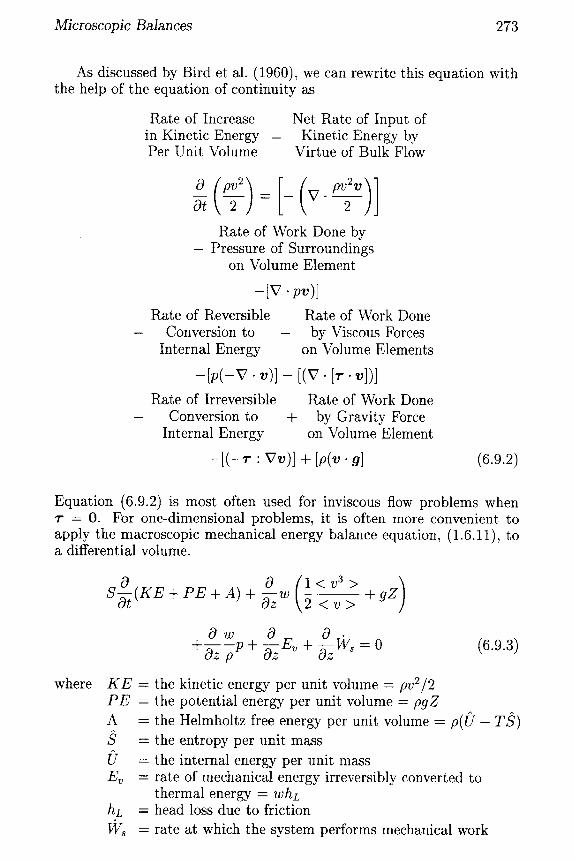
As discussed by Bird et al. (1960), we can rewrite this equation with the help of the equation of continuity as
Rate of Increase in Kinetic Energy Per Unit Volume
Net Rate of Input of Kinetic Energy by
Virtue of Bulk Flow
[ Rate of Work Done by
- Pressure of Surroundings on Volume Element
-[v. pv)] Rate of Reversible Rate of Work Done
Conversion to - by Viscous Forces Internal Energy on Volume Elements
- [ p ( - V . v)] - [ (V-[~-v] ) ]
Rate of Irreversible Rate of Work Done Conversion to + by Gravity Force
Internal Energy on Volume Element
- [ ( -7"" Vv)] + [p(v. g] (6.9.2)
Equation (6.9.2) is most often used for inviscous flow problems when 7- = 0. For one-dimensional problems, it is often more convenient to apply the macroscopic mechanical energy balance equation, (1.6.11), to a differential volume.
where
O ( 1<v3> ) S-~O ( K E + P E + A ) + --~z w -2 < v > + g Z
O w 0 0 + -~z p p + ~z Ev + -~z ~ ~ - 0 (6.9.3)
K E - the kinetic energy per unit volume - pv2/2 P E = the potential energy per unit volume = pgZ A
hL
- the Helmholtz free energy per unit volume - p ( U - TS)
- the entropy per unit mass
- the internal energy per unit mass = rate of mechanical energy irreversibly converted to
thermal energy = W hL = head loss due to friction
= rate at which the system performs mechanical work
274 Computational Methods for Process Simulation
S
= w ~ = work performed per unit mass - cross-sectional area
6 . 1 0 P I P E L I N E G A S F L O W
Here we want to consider the flow of a compressible gas down a pipe at steady state.
The equation of continuity is
w = constant (6.10.1)
and the mechanical energy balance is
- - - p + - 0 dz p
Assuming p does not vary with distance to the extent that pressure does gives
wdp d ( l v 2 z f ) pd--~ + w d z 2 4D - 0 (6.10.3)
where f is the friction factor. For turbulent flow f is constant. Also v does not vary significantly with z; therefore,
@ v2pf d--~ = 8 0 (6.10.4)
and introducing the volumetric flow rate F, we have
vT~ D 2 F = 4 (6.10.5)
The mechanical energy balance equation, (6.9.3), then becomes
@ 2 F2p d--~ = - f - ~ D---/- (6.10.6)
The equation of state for an ideal gas is
p(mw) ( 6 . 1 0 . 7 ) P - RT
The information-flow diagram for solving this problem is shown in Fig- ure 6.4.

Microscopic Balances 275
f D
p( z = O) [ F 2 initial ~1 dp 2 p condition [ d-zz = - f ~ Ds
p _. p(mw) RT
. .4-.--mw
-~---RT
142 F = - p w = constant
F i g u r e 6.4: P i p e l i n e G a s F l o w .
6.11 D E V E L O P M E N T OF M I C R O S C O P I C T H E R M A L E N E R G Y B A L A N C E A N D ITS A P P L I C A T I O N
The conservation law for total energy is
Rate of Accumulation Rate of Internal of Internal and = and Kinetic Energy Kinetic Energy In by Convection
Rate of Internal - and Kinetic Energy
Out by Convection
Net Rate of Net Rate of Work + Heat Addition - Done by the System (6.11.1)
by Conduction on the Surroundings
This statement is not complete for it neglects nuclear terms, radia- tion terms, electromagnetic terms, and reaction terms. This later reac- tion term must often be included in chemical engineering problems as a generation term.
The accumulation of total energy in the differential volume AxAyAz is
0 1 2 O--~ (P(J +-~pv ) AxAyAz
where U is the internal energy per unit mass and v is the magnitude of the local fluid velocity. The convective terms are
v~(pU + 1/2pv2)~XzAy I~ -v~(pU + 1/2pv2)~Xz~Xy I~+~

276 Computational Methods for Process Simulation
+ vy(p(f + 1/2pv2)AxAz ly -vy(pU + 1/2pv~)AxAz I~+~y + Vz(p~I + 1/2pv2)AxAy [z-v~(p5 + 1/2pv2)AxAy Iz+~
The conduction terms are
q~AyAz I~ -q~AyAz I~+p,~ + qyAxAz ly -qyAxAz ly+A~ + qzAxAy Iz -qzAxAy I~+Az
where q~, qy, and q~ are the components of the conductive heat flux vector q.
The work done by the fluid element against its surroundings consists of work against volume forces (gravity) and work against surface forces (pressure, viscous). The gravity term is
the pressure term is
pAxAyAz(v~gx + vygy + Vzg~)
pv~AyAz I~ -pv~AyAz I~+A~ + pvyAxAz ly -pvyAxAz ly+Ay + pvzAxAz tz-pvzAXAy Iz+~z
and the viscous terms are
~y~z(~,~v~+~,~v~+~zVz) I , -~y~z(~ ,v ,+~ ,~v~+~z~z) I,+~ + ~ ~ z ( ~ ~ + ~ ~ + ~ z ) t ~ - A ~ A z ( ~ ~ + ~ ~ + ~ ~ ) I~+~ + AxAy(T~xv~+~'zyV~+%zVz)Iz--AxAy(7~xvx+TzyVy+TzzVz) Iz+Az
Dividing by the volume element and taking the limit as AxAyAz goes to zero gives
0 + 1 1 2 0 lpv2)
o l v )l (oq oqz) + Kz v~ (PU + ~ -~x + N + -OS-z
o o ) + (p(v~g~ + vygy + Vzgz)- pv~ + Npv~ + Npvz
[o o - N(~-~xV~ + ~ - ~ + ~-~zVz) + N ( ~ - ~ + ~-~v~ + ~-~zV~)
o 1 + -~z(Tz~V~ + ~-xyv~ + rzzV~) (6.11.2)
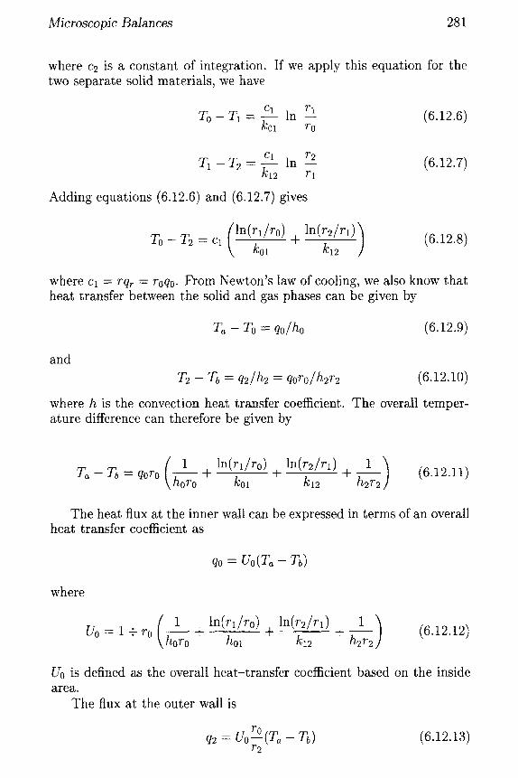
Microscopic Balances 277
This is the equation for the conservation of total energy. Subtracting the mechanical energy equation (6.9.2) from equation (6.11.2) gives the thermal energy equation
DO PDT : -(V-q) - p(V. v) - T" Vv) (6.11.3)
Putting in the thermodynamics relation for the internal energy
d O - - ~ d ~ ' + ~ ? d T (6.11.4)
gives
P D t - - p + T ~ p D---~ (6.11.5)
When included in the thermal energy equation, we get the thermal energy equations given in Tables 6.7, 6.8, and 6.9 for various geometries.
Table 6.7: Components of the Energy Flux q (Source: Bird et al., 1960)
Rectangular Cylindrical Spherical
OT OT OT q~ - - k - - ~ q~ - - k q~ - - k
Or Or o x
OT - - k I OT I a T qy - -k--~_. qe qo - - k - - -
r 00 r 00 ely
OT OT 1 0 T qz - - k - ~ z qz - - k - ~ z q , - - k ~ r sin 0 0¢
6.12 H E A T C O N D U C T I O N T H R O U G H C O M P O S I T E C Y L I N D R I C A L W A L L S
We are interested in computing the steady-state heat flux for conduction through composite material cylindrical walls. A diagram of the system is given in Figure 6.5.

278 Computational Methods for Process Simulation
Table 6.8" Equation of Thermal Energy in Terms of Energy and Momentum Fluxes (Source: Bird et al., 1960)
Rectangular coordinates" p~v(OT OT OT OT) -~ + v~N + ~ N + ~zN -
(oq~ 0% O~z~ (~) ~ov~ ov~ Ovz) - -~ +97 + a ~ ) - r 'ka~ + 9 7 + - 5 ;
{ 0. 0v~ 0~z} { (0. 0v~) - ~ - ~ x + ~ - ~ v + ~ z z - ~ z - ~ -~y +-aTx (av~ a~z)(av~ a~)} +~= -OVz + ~ - +~z -aT+-b7
Cylindrical coordinates: p(;v( aT aT voOT aT) - g + ~ ~ ~ ~ ao ~ V z ~ -
r -~r rq" + - + - T - rv~ - - ~ N . - ~ ~ ~ ~
- r~Or
l Ovo Ov~ ~ tO0 ~ Oz]
1 ( O v o ) OVz} { [ 0 ( ? ) 10v~] rOO-r \00 + v~ + r z z ~ - ro~ r-&r + -r OO J
+~-~z --~ + oz ] + ~-o~ - - f ig+ -~z
coordinates" p~, ( OT OT Spherical -b7 + ~ T e k
ve OT v¢ OT'~ tO0 t ) r sin O 0¢
1 0 2 1 (9 1 Oq¢ - 7 5 - ~ r r q~ -~ (qo sin O) -~ r sin 0 00 r sin 0 00 ]
(019) [1~_7r 1 0 1 ave] - T -~f ; -~ r2v, q (vesinO)-~ r sin ~9 00 r sin O 0¢
{ o~ (~ovo ~) (1 ovo Vr - r~--oT+r°° ---~-+r +r , , rsinO 0¢ ~---+r
{ ~ov~ ~o~ (~ - r~o ~ +r~, -~r~
r O~ r
r sin 0 0 ¢ r
1 Ovr r sin 0 0¢
v0cot0) } r
r
Note: The terms contained in braces {} are associated with viscous dissipation and may usually be neglected, except for systems with large velocity gradients.

Microscopic Balances 279
Table 6.9" Equation of Thermal Energy (for Newtonian Fluids with Constant p, #, and k) (Source: Bird et al., 1960)
Rectangular coordinates:
- ~ + v ~ N + v ~ N + V z N - k - ~ + N~y~ + -~z~
{(Ovx Ovz) +" -g-jy + O x ) + \ O z + -gx + +5-{
Cylindrical coordinates"
pCv --~ + v~-sr ~ ~-Vz - k - r -~ r O0 -~z r ~ -~r r 2 0 0 2
+2. o~ ] + \ oo + ~ + \ o~ +" 7 2 + ; oo ]
[ (OVz OVr~ 2 l OVr 0 Vo + \o~ + Oz) + 7 - g + ~ P
Spherical coordinates" ( OT OT v o OT v ¢ OT )
pdv -g-( + v ~ ~ t - r 00 r sin 0 0¢ [1 0 ( O T ) 1 cO ( c O T ) 1 02T]
k V ~ ~ -~r + r 2sin000 sin O N +r2sin20~-5]
Ov~ ~ 2 l Ovo 1 0% Vr +2~ O r ] + - + - - + ~- - - + r ~ r r sin 0 0¢ r
{[ 0 ( ? ) l Ov~] 2 [ 10v~ 0 ( ? ) ] +# rorr + r 0 0 J + rsinO0¢ ~-r-~r
[sin00 ( v ¢ ) 10vo] 2} + r cO0 sin0 rsin0O0
02T]
2
v°c°tO) 2 } r
2
Note: The terms contained in braces {} are associated with viscous dissipation and may usually be neglected.

280 Computational Methods for Process Simulation
z Fluid at temperature T b
Fluid at temperature T a
T a T 0 T 1 T 2
Figure 6.5" H e a t C o n d u c t i o n T h r o u g h C o m p o s i t e Cy l ind r i ca l Walls.
By writing an energy balance for the solid over a differential volume element 27rrArL, we get
Rate of = Rate In - Rate Out Accumulation
0 - q~27rrL [~ -q~2~rrL I~+ZXr
Dividing by Ar and taking the limit as Ar --+ 0 gives
(6.12.1)
drqr dr
which, upon integration, becomes
= 0 (6.12.2)
rqr -- constant - cl
Using Fourier's law of heat conduction we have
(6.12.3)
dT -rk- r
which, upon integration, gives
- - C 1 (6.12.4)
c1 T - ~-ln r + c 2 (6.12.5)
Microscopic Balances 281
where c2 is a constant of integration. If we apply this equation for the two separate solid materials, we have
cl in r~ (6.12.6) To - T~ = k01 r0
Cl ?"2 r l = i n -
r l (6.12.7)
Adding equations (6.12.6) and (6.12.7) gives
ln(rl/ro) To - T 2 - Cl k01
ln(r2/r~)) (6.12.8) + k12
where ca - rqr - roqo. From Newton's law of cooling, we also know that heat transfer between the solid and gas phases can be given by
T~ - To = qo/ho (6.12.9)
and
T2 - Tb -- q2/h2 - qoro/h2r2 (6.12.10)
where h is the convection heat transfer coefficient. The overall temper- ature difference can therefore be given by
T ~ - T b - q o r o ( ~ o r ° ln(r2/rl) 1 ) ln(rl/ro) + + (6.12.11)
+ kol k12 h2r2
The heat flux at the inner wall can heat transfer coefficient as
be expressed in terms of an overall
qo - Uo(T~ - Tb)
where
1 ln(rl/ro) ln(r2/rl) 1 ) - - + + + (6.12.12)
Uo 1 + ro horo hol k12 h2r~
U0 is defined as the overall heat-transfer coefficient based on the inside area.
The flux at the outer wall is
q2 - Uo r° (Ta - Tb) (6.12.13) 7"2
282 Computat ional Methods for Process Simulation
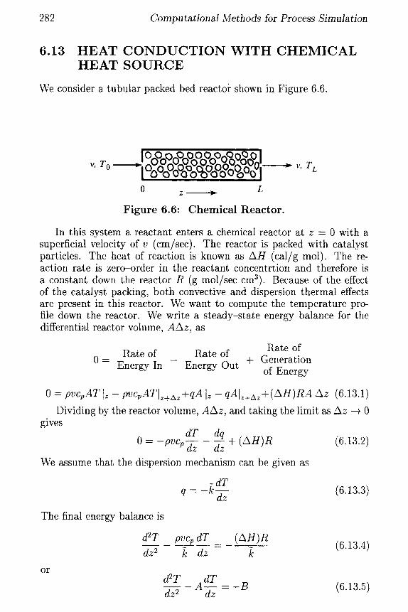
6.13 H E A T C O N D U C T I O N W I T H C H E M I C A L H E A T S O U R C E
We consider a tubular packed bed reactor shown in Figure 6.6.
v, TO ~ , . ¢ . , , . , v _ ~ _ v _ _ v , . , 7 . , v . . = v v n - .
go 03 0 L
"- v , T L
Figure 6.6: Chemical Reactor.
In this system a reactant enters a chemical reactor at z = 0 with a superficial velocity of v (cm/sec). The reactor is packed with catalyst particles. The heat of reaction is known as AH (cal/g tool). The re- action rate is zero-order in the reactant concentrtion and therefore is a constant down the reactor R (g mol/sec cm3). Because of the effect of the catalyst packing, both convective and dispersion thermal effects are present in this reactor. We want to compute the temperature pro- file down the reactor. We write a steady-state energy balance for the differential reactor volume, A A z , as
Rate of Rate of 0 - Energy In Energy Out
Rate of + Generation
of Energy
0 - pvcpAT iz - pv%ATIz+Az+qA [z - q A I z + A z + ( A H ) R A A z (6.13.1)
Dividing by the reactor volume, A A z , and taking the limit as Az --+ 0 gives
dT dq 0 - -pVCp dz dz ~- (AH)R (6.13.2)
We assume that the dispersion mechanism can be given as
q _ _ ~ d T dz (6.13.3)
The final energy balance is
~ T pvcp dT (AH)R
dz 2 k dz (6.13.4)
OE
d2r A dT _ - B (6.13.5) dz 2 dz

M i c r o s c o p i c B a l a n c e s 283
with
A - p v % . . . . and B - (AH)R (6 13 6) k k
As boundary conditions for the problem we assume that we know the inlet reactor temperature
T ( z - O) - To (6.13.7)
and we know that once we leave the reactor, the temperature will remain constant, so
d T dz (z - L) - 0 (6.13.8)
The differential equation of (6.13.5) is a linear second-order, nonho- mogeneous equation. From Appendix A we find that the homogeneous solution is
Th -- C l e Az + C2 (6.13.9)
where C 1 and C2 are constants of integration. The particular solution is
B Tp - --~z (6.13.10)
The general solution is therefore
B T - C1 eAz + ---~z + C2 (6.13.11)
Using the boundary conditions of (6.13.7) and (6.13.8) gives
TO -" C1 -~- C2 (6.13.12)
B -AL (6.13.13) C1 = - A---Te
The final temperature profile is calculated as
B B (e_AL T - To + ---~z + - ~ - e -A (L - z ) ) (6.13.14)
6.14 M A T H E M A T I C A L M O D E L I N G F O R A S T Y R E N E M O N O M E R T U B U L A R R E A C T O R
We desire to develop a mathematical model for a styrene monomer pilot plant. The process flow sheet is shown in Figure 6.7. Ethylbenzene is passed through a tubular reactor packed with an iron oxide catalyst, and

284 Computational Methods for Process Simulation
dehydrogenation to styrene takes place. The ethylbenzene feed stream is preheated and mixed with superheated steam to a reactor inlet temper- ature of over 875 K. Since the dehydrogenation reaction is endothermic, there is a temperature drop of as much as 50 K down the reactor. The residence time of the gas stream in the reactor is typically one second. Superheated steam serves as a diluent, decokes the catalyst extending its life, and supplies sensible heat to keep up the reaction temperature. There are by-product reactions which produce benzene and toluene along with lighter components, methane and ethylene. The latter two can react in water-gas shift reactions to produce more hydrogen, carbon monoxide, then carbon dioxide. A list of the significant chemical reactions appears in Table 6.10. There are ten distinct chemical species, and the ra~e of reaction, that is, rate of disappearance, of each species is described in Table 6.11. Kinetic expressions have been developed for each reaction rate (Sheel and Crowe, 1969; Wenner and Dybdal, 1948; Clough and Ramirez, 1976) and are given in Table 6.12.
~FF- GAS
SUPERHEATER ~ SEPARATOR
STEAH 11025 K _ 800K FEE~'--D~ 1925K " LCROOE STYRENE
PRODUCT ~ S T E A N
CA TAL YTIC OONDEH SATE REACTOR ETHYL-
BENZENE FEED
Figure 6.7: Styrene Pilot Plant.

Microscopic Balances 285
Table 6.10" Significant Chemical React ions
C6HhCH2CH3 ~ C6HhCHCH2 + H2 (ethylbenzene) (styrene)
C6 Hh C H2 C H3 --+ C6H6 + C2H4 (ethylbenzene) (benzene) (ethylene)
C6 Hh C H2 C H3 + H2 ~ C~ Hs C H3 + (ethylbenzene) (toluene)
H2 0 + 1//2 C2H4 -+ CO + (ethylene)
H20 + CH4 --+ CO (methane)
÷
CH4 (methane)
21-12
H20 + CO ~ C02 +
3 ~
Table 6.11" Ra tes of D i sappea rance
Species Reaction rate (R j)
1 Ethylbenzene R1 + R2 + R3 2 Styrene - R1 3 Hydrogen - R1 + R3 - 2 R 4 - 3R5 - R6 4 Benzene - R2 5 Toluene - R3 6 Methane - R3 +R5 7 Ethylene - R2 + 1//2 R4 8 Carbon monoxide - R 4 - R5 + R6 9 Carbon dioxide - R6
10 Water R4 + R~ + R6
We will develop an appropriate mathematical model for the pilot scale reactor studied by Clough and Ramirez (1976). The mathematical model is derived by simplification of the general conservation equations. The re- duction of the general equations is made possible by order-of-magnitude scaling agreements based upon reasonable values for system dependent and independent variables. An important approximation which is im- plied in the model development is that the flow through the packed bed reactor can be described by both axial and radial dispersion mechanisms.

286 Computational Methods for Process Simulation
Table 6.12" React ion Kinet ics Express ions
Ethvlbenzene dehydrogenation kl =R~'Tw~ exp(F1 - E 1 / R g T )
R1 -- k l (C~ - C 2 C 3 / I ~ e )
Dealkylation to benzene
R2 = k2C1
Dealkylation to toluene
R3 = k3C, C3 Water-ethylene shift
R 4 : k 4 C l 0 v ~ 1
Water-methane shift
R5 : k5C6C10
Water-carbon monoxide shift P
I~6 -- k668C10 RgT
K~=R-- ~ exp(16.12 - 15350/T)
Rg Twe k2= po exp(13.24 - 49675/RgT )
p~ ] CO e exp(0.2961- 21957/RgT)
k4~_(RgT~ 3/4 p~ ] 03 e exp(-O.O724-24838/RgT)
po ] a~ exp( -2 .934-15697/RgT)
R_~ 3 ~ exp(21.24 - 17585/RgT )
w~ = catalyst weight per reactor void volume
6.14.1 Gas Phase Energy Balance
We first start with the general thermal energy balance for the fluid phase within the reactor,
pCv DT (OP) ( V . v ) - ( ' r ' W v ) ( 6 . 1 4 . 1 ) D---~ = - ( V " q) - T ~
For an ideal gas
and assuming viscous dissipation effects are negligible gives
(6.14.2)
DT pC~ Dt : - ( V . q) - p ( V . v) (6.14.3)
We need to add the local sources and sinks of thermal energy to this equation:
Q~ = heat transfer between the catalyst and fluid phases Q~ = heat of reaction
This gives for the general thermal energy balance
DT pCv D---t- = - ( V . q) - p ( V . v) + Q~ + Q~ (6.14.4)
Microscopic Balances 287
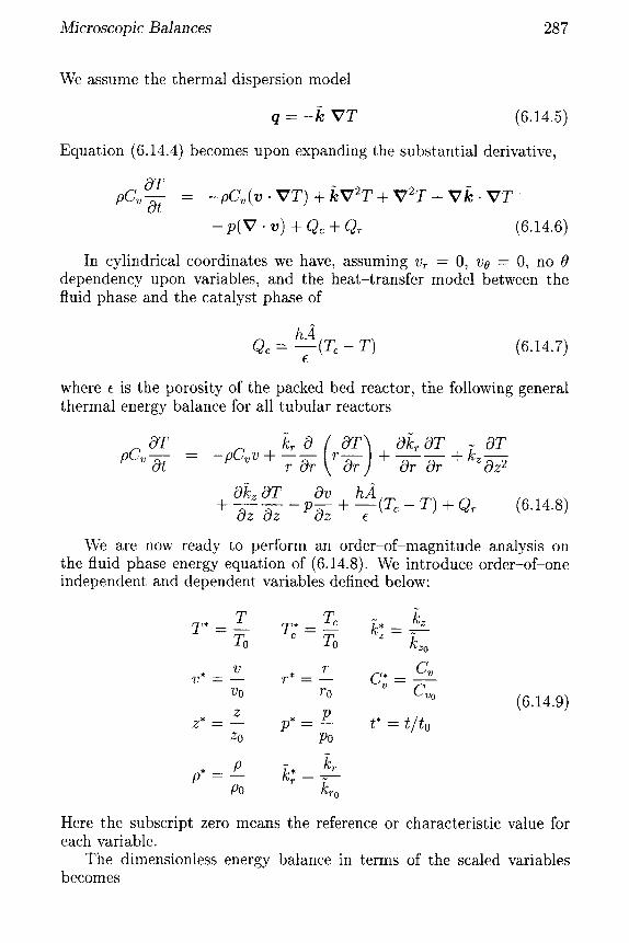
We assume the thermal dispersion model
q - - k VT (6.14.5)
Equation (6.14.4) becomes upon expanding the substantial derivative,
OT pCv Ot = - p C ~ ( v . V T ) + ]~V2T + V 2 T + V i e . V T
- p ( V . v) + Q~ + Q~ (6.14.6)
In cylindrical coordinates we have, assuming v~ - O, vo - O, no 0 dependency upon variables, and the heat-transfer model between the fluid phase and the catalyst phase of
h~4 Q ~ - ( T ~ - T ) (6.14.7)
where e is the porosity of the packed bed reactor, the following general thermal energy balance for all tubular reactors
_ l o g O ( r O T ) O[c~OT OT ~Cv OT - pCv v + - - ~ ~ k z
Ot - r ~ -~r Or Or Oz 2
O[Cz o r Ov hA t Oz Oz P-~z + ~(T~e - T ) + Q~ (6.14.8)
We are now ready to perform an order-of-magnitude analysis on the fluid phase energy equation of (6.14.8). We introduce order-of-one independent and dependent variables defined below"
T T~ - k z T*=T0 T;=~ L=Lo
v r C~ v* : ~ r* = - - C v =
YO 7"0 Cvo z* - - z p, _ - P t* - t / to
Zo Po
P*--P k r - kr po k~o
(6.14.9)
Here the subscript zero means the reference or characteristic value for each variable.
The dimensionless energy balance in terms of the scaled variables becomes

288 Computational Methods for Process Simulation
(ToPoCvo) p, OT* (poC~ovoTo) p,C~v, OT* -to C~ Or* = - zo Oz*
+ ] + Or*
+ z2 ° k~oz,2 -~ Oz* Oz* ,, zo / Oz* Tohf~
+ (T~-T*)+Qr 6_.
(6.14.10)
To prepare an order-of-magnitude analysis on various terms within the fluid thermal energy balance (6.14.10), all terms will be compared to the convective term. We therefore divide all terms by (p°c~°È°T°)
Z0
zo ) p, OT* C or,
( zo)a zOT* + zopo----C~ovo Oz* cgz*
p0V~oT0 87* +
= -p*Cvv* OT* kzo -, + zopoC~ovo kz Oz,2
~- r~po~--C~ovo [ r* Or-----: r* Or, ]-~
zohft ) ( r e _ T , ) epoCvovo
Ok~ aT*] Or* Or:
(6.14.11)
All leading coefficients are dimensionless except the last. This is because the heat of reaction has not been made dimensionless since it is a complex function of the other system variables. The entire last term (in braces) is dimensionless and needs to be retained in the process model since the endothermic heat of reaction is an important process mechanism.
Typical pilot plant conditions for the specific reactors studied by Clough and Ramirez (1976) are given in Table 6.13.
Using these characteristic values, the dimensionelss coefficients can be calculated and are used to help eliminate the less important terms of equation (6.14.11). The coefficients are
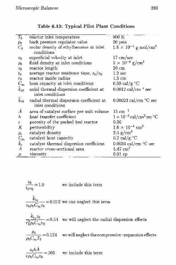
Microscopic Balances 289
Table 6.13: Typical Pilot Plant Condit ions
To Po Co
Vo Po Zo to ro Cvo kzo
A h
K
pc
kc A #
reactor inlet temperature back pressure regulator value molar density of ethylbenzene at inlet
conditions superficial velocity at inlet fluid density at inlet conditions reactor length average reactor residence time, zo/vo reactor inside radius heat capacity at inlet conditions
axial thermal dispersion coefficient at inlet conditions
radial thermal dispersion coefficient at inlet conditions
area of catalyst surface per unit volume heat transfer coefficient porosity of the packed bed reactor permeability catalyst density catalyst heat capacity catalyst thermal dispersion coefficient reactor cross-sectional area viscosity
900 K 20 psia 1.8 × 10 -4 g mol/cm 3
17 cm/sec 5 × 10 -4 g/cm 3 20 cm 1.2 sec 1.3 cm 0.59 cal/g °C 0.0012 cal/cm o sec
0.00023 cal/cm °C sec
-1 15 cm 1 × 10 -3 cal/cm 2 sec °C 0.36 1.6 × 10 -4 cm 2 2.4 g/cm 3 0.2 cal/g °C 0.0034 cal/cm o C sec 5.47 cm 2 0.01 cp
Z0
to Vo ~ = 1 . 0 we include this term
kzo zopoC, ovo
=0.012 we can neglect this term
kro Zo r~poC~oVo
=0.54 we will neglect the radial dispersion effects
Po poC oTo
=0.124 we will neglect the compression-expansion effects
zohA cpoVvovo
= 166 we include this term

290 Computational Methods for Process Simulation
The scaled equation for this reactor is therefore
OT* -p* Cv v* OT* T* p'C; Ot* = ~-7z* + 166(T2 - ) + {4.43Q~} (6.14.12)
6.14.2 C a t a l y s t Bed E n e r g y B a l a n c e
We now develop the solid phase catalyst bed thermal energy equation. Since the catalyst bed is stationary, the general energy balance becomes
p c C ~ O T ~ - - ( V ' q ) - ( e ) - 1 - e (6.14.13)
which in cylindrical coordinates is expressed as
Ot = k~-~z2 + -r -~r - 1 e Qc (6.14.14)
The dimensionless scaled equation becomes
to Ot* - z~ Oz .2 + r~ r'Or* r* . . . . .
- 1 - e (T~* - T*) (6.14.15)
We normalize the equation with respect to the last term. This gives the dimensionless coefficients,
p~@~(1- e) = 17 we include this term tohft
k~(1 - e) = 0.0004 we neglect the axial dispersion term z hA
kc(1 - ~) = 0.09 we will include the radial dispersion term
The final scaled catalyst thermal energy balance is
170T~-0 .091 0 (r *OT~) T* Ot* r--i-~r * ~ - (T~ - ) (6.14.16)
We can now compare the relative time scales for the gas phase and catalyst phase balances. To do this, we normalize the gas phase balance by the heat transfer term so that both catalyst and gas equations are normalized by the same term. This gives
OT* OT* T* 0.00602p*C~ Ot* = -O'O0602p*C~v*-~z* + (re* ) + {0.0267Q,}
(6.14.17)

Microscopic Balances 291
Comparing the leading coefficient of the two accumulation terms shows that the ratio of the fluid dynamics to the catalyst dynamics is
~-f = 0.00602 = 3.54 x 10 . 4 (6.14.18) Tc 17
This means that the dynamic response of the fluid phase is much faster than that of the catalyst temperature response.
6.14.3 Equation of Motion
The general equation of motion or momentum balance is
0 Ot (pv) - - V . pvv - V p - V . r + pg (6.14.19)
which in cylindrical geometry is
10TOz O'rzz ) 0 0 0t) 1 0 (r )-t (6.14.20) o-7 ( '°vz) - Oz Oz r r O0 Oz
For flow through a packed bed, the viscous terms are given by Darcy's law
( l OTOz OTzz ) # 1 0 (r r~z)~ ~ - (6 14.21) -i-g r O0 Oz -~Vz .
where K is the permeability of the packed bed. Therefore the equation of motion is
o o op # O---i (pvz) - Oz (pv2z) Oz K vz (6.14.22)
Using the Equation of Continuity
Op 0 0--[ = Oz (pvz) (6.14.23)
gives OVz Ovz 1 Op # Ot = -Vz Oz p Oz p--~Vz (6.14.24)
Scaling and normalizing with respect to the convective term yields
- ~ Oz---: - v~po p* Oz* KroPo -fi: (6.14.25)
Using typical values gives for the coefficients
z0 = 0.98 #Zo = 1.36 x 10³ P0 = 9.5 x 10⁶ (6.14.26) to vo K vo po v~) po

292 Computational Methods for Process Simulation
The values imply that the pressure coefficient dominates the momen- tum balance and therefore
Op* = 0 (6.14.27)
cOz* o r
p* - constant (6.14.28)
6.14.4 Materia l Balances
The component material balances in cylindrical geometry are
O(VzC ) Dr 0 ( O Ci Ot ~ Oz = r Or r or ] + D z Oz 2 R~ (6.14.29)
i=1, N where N - number of chemical species
Using characteristic values, the scaled dimensionless equation is
~o t o o r * - - O z - - - - - - z - - v o C--~o
o r
0C~ _ O(v*C~) { z0Ri } (6.14.31) 0.98 Ot* - - - Oz* - voCo
6.14.5 S t e a d y - S t a t e M o d e l So lu t i on
We want to compute the steady-state temperature and composition pro- files for the styrene tubular reactor. The final model equations are
o - - p C p v OT ~ z + Q~ + Qr (6.14.32)
r Or r Or ] - Q~
O(vCi) 0 - - o---7-- - R~ ( 6 . 1 4 . 3 4 )
At any axial position z, the value of the fluid temperature T is a constant and not a function of radial position. This is because equations (6.14.32) and (6.14.34) only have axial derivatives and no radial deriva- tives appear. This means that we can solve for the catalyst temperature from equation (6.14.33) since it is only a function of the radial position.
Equation (6.14.33) can be solved analytically for the catalyst tem- perature at any axial position as a function of radial position. The differential equation is
d
d~ ~ - ~ V / - (1 - ~----]

Microscopic Balances 293
with the boundary conditions
dT~ dr
= 0 at r - 0 (6.14.36)
If we make the following substi tut ions
at r - R (6.14.37)
r T ~ - T R2hft - -- Y - /32 - (6.14.38)
s R T~ - T - k~(1 - e)
then d2y 1 dY
¢t2Y - 0 (6.14.39) ds 2 s ds
with dY
ds = 0 at s - 0 (6.14.40)
Y - 1 at s - 1 (6.14.41)
This is a Modified Bessel Equat ion (Wylie, 1960) which is a special linear second-order differential equation with nonconstant coefficients. The solution is given as
v(~) - c'1 io ( /~)+ c~ Ko(/3~) (6.14.42)
where
E k=O
K. (~) - I,, (x) f
Using the s - 0 boundary condition
/ k ! (k+p) ! (6.14.43)
dx
x I~(x) (6.14.44)
dY O -
ds
, dlo dKo -- Cl-'~8 + C; -~8 (6.14.45)
It has been shown (Wylie, 1960) that
d d-~ ~o(X) - ~_~ (x) (6.14.46)
and d
dx Ko(x) - - K - l (X) (6.14.47)
A l s o J - l ( 0 ) - 0 a n d K _ 1 (0) - (:x)
Therefore the s - 0 boundary condition implies tha t C~ - 0

294 Computational Methods for Process Simulatiou
A t s - 1 Y - 1 - C'~ / o ( / 3 )
Therefore, the general solution is
(6.14.48)
Y ( s ) - Io(13s) (6.14.49) ~o(9)
or
Io ~(1-~1 (T~ - T) - R] (T~o - T) (6.14.50)
I0 i~o(hA )
We can now integrate the gas phase energy balance (6.14.32) over the radial cross-sectional area for flow,
Ae - 7rR2~ (6.14.51)
or
This gives
d a - 2~rer dr (6.14.52)
-(pCpv)--~zda + ~ ( T ~ - T)da + Q~ da - 0 (6.14.53) e c 6. e
or
dT -¢~n~(pC, v ) ~ j~0 R + 27~ hA(Tc - T)r dr + CTrR2Qr - 0 (6.14.54)
Actually at r - R an additional heat source must be considered. This is the heat transfer between the fluid and the exposed reactor wall. This can be modeled as
Qw - h~A~(T~ - T) (6.14.55)
where h~ is the heat transfer coefficient and A ~ is the exposed wall area. We can now use our analytical solution for T~ as a function of radial
position to evaluate
fo~(T~- T)< d< - (T~ - T) fo ~ Io(¢R) Io(~r)r dr (6.14.56)
with
I hA ~- ~(~ _ ~) (6.14.57)
Microscopic Balances 295
Again using the properties of Bessel Functions (Wylie, 1960), we get
R I~ (R¢)(Tw - T) (6 14.58) ~(Tc - T)r a~ - ~/~ I0(R¢)
The fluid energy therefore
balance integrated over the radial cross-section is
-pGvdT-~z + [ 2cRv~ Io (R¢)II(R~)] h~(Tw - T) + Qw + Qr - O
or J -pCpv dT + (h.4Zr + h ~ A ~ ) ( T ~ - T) + q r -- 0
where/3~ is an effectiveness factor defined as
(6.14.59)
(6.14.60)
2 I1 (R~) /3~- ~R¢ Io(R~2) (6.14.61)
Equation (6.14.60) can now be integrated with the material balance equation
d(~C~) = -R~ (6.14.62) dz
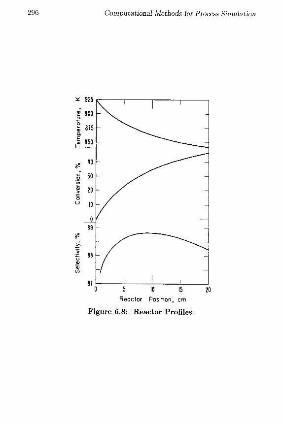
With the boundary conditions that the inlet temperature and inlet compositions are known, these equations can be integrated numerically using the IMSL numerical integration routines introduced in Chapter 4. Typical numerical results obtained by Clough and Ramirez (1976) are shown in Figure 6.8. Here we observe the temperature drop down the reactor due to the endothermic dehydrogenation reactions, the steady monotonic rise in styrene conversion down the reactor (styrene concen- tration per initial ethylbenzene concentration), but an internal maximum in the styrene selectivity (styrene concentration/styrene concentration + benzene concentration + toluene concentration). With this model it is possible to perform an optimization study for the reaction system to maximize profitability. Profitability is defined as the value of the prod- uct styrene minus the loss in profit caused by producing by-products, minus the utility cost of generating steam. Such an optimization study has been performed by Clough and Ramirez (1976), who showed that the major control for the reactor is the steam-to-ethylbenzene ratio.
296 Computational Methods for Pro('cs,~' SillJalh~,t,i~ta
~' 925
900 1 . _
0 ' - 815 Q.
E 850
t 1 '
4O
c" 30 0
h .
® 20 ¢-
0
0 89
. _
= 88 U
81 i 0 5 I0 15
Reactor Position, cm
F i g u r e 6.8" R e a c t o r Prof i les .
20
Microscopic Balances 297
P R O B L E M S
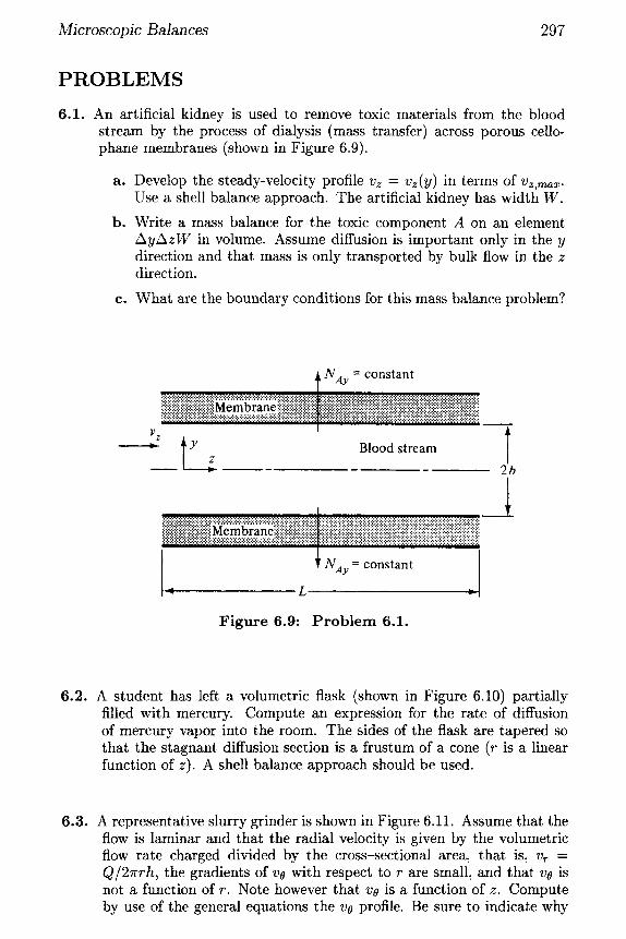
6.1. An artificial kidney is used to remove toxic materials from the blood stream by the process of dialysis (mass transfer) across porous cello- phane membranes (shown in Figure 6.9).
a. Develop the steady-velocity profile Vz = vz(y) in terms of Vz,max. Use a shell balance approach. The artificial kidney has width W.
b. Write a mass balance for the toxic component A on an element A y A z W in volume. Assume diffusion is important only in the y direction and that mass is only transported by bulk flow in the z direction.
c. What are the boundary conditions for this mass balance problem?
t NAy = cons tan t
.... : : .................................. ........... iti ............................ iiiiiiiiiiiiiiiiiiiiiii ii !iiii !i iiiiiNiii i i i m:i ; : i!i i! !i Ni i i iiNN!iNiii i i i3i Ni i!i iNNi i i!i i i i iii i!iii! l, z I
- - - - -~ . . . . . . ~ z Blood stream
I
~:::~::::~:~i::~:~:~..~.~:~:~:~:~:~:~:~:~:~i~!~i~i~i~i~!i~I~!~i~i!i!i~.~.~!~.~.~.~.~.~.~.~.~.~.~.:.~.~.~.~.~.~.:::::::::::::::::::::::::.~.~.~.~.~.~
- ~ ' I . , .....
Figure 6.9" Problem 6.1.
2b
6.2. A student has left a volumetric flask (shown in Figure 6.10) partially filled with mercury. Compute an expression for the rate of diffusion of mercury vapor into the room. The sides of the flask are tapered so that the stagnant diffusion section is a frustum of a cone (r is a linear function of z). A shell balance approach should be used.
6.3. A representative slurry grinder is shown in Figure 6.11. Assume that the flow is laminar and that the radial velocity is given by the volumetric flow rate charged divided by the cross-sectional area, that is, vr = Q/21rrh, the gradients of ve with respect to r are small, and that ve is not a function of r. Note however that ve is a function of z. Compute by use of the general equations the v6 profile. Be sure to indicate why

298 Computational Methods for Process Simulation
z o / ( Sg
Figure 6.10: P r o b l e m 6.2.
you can eliminate the appropriate terms. You should be able to show that
d2V° -Evo where E - (1 QP ) dz 2 - ~ + 27rr 2h#
Solve this differential equation with the appropriate boundary condi- tions.
Charge
i otor I
Discharge ~ ~
F igure 6.11" P r o b l e m 6.3.
6.4. Prove that the forms of Fick's law given in equations (6.2.6) and (6.2.9) are equivalent.
6.5. Temperature Profile in a Porous Reactor Tube
Figure 6.12 shows a schematic representation of a porous tubular reac- tor. The reactant gas and diluent enter the pores of the tube and flow radially towards the center of the tube. Heat is generated in the solid by means of a constant electric current flowing through the solid, and heat is removed by the endothermic reaction.

Microscopic Balances 299
Quench S t ream
r o ~ . . . _ . . _ . . . _ . .~
r i Graphi te Washer
\,i 1:. . . . .
Reactant ........ ~: ~2:.'i:!~:.:.'::(i: fi;-:-i:?ii~i + Diluent f!!/i.--::(-:::
l-)"iJ~!i~: ~-!:!.~! ~'~ l!~!~-~..--->~
i
F i g u r e 6 .12 :
P r o d u c t + Quench S t r e a m
P o r o u s T u b e R e a c t o r .
Write differential thermal energy balances on both the solid phase and the gas phase in the porous reactor.
You can assume
1. J -- a constant volumetric rate of heat generation in the solid due to electric current, ca l /hr m 3.
2. The heat- transfer rate per unit volume between the solid and gas phase can be modeled by use of a heat- t ransfer coefficient, h
Q = ha(T2 - TI)
where a = surface area per volume of porous reactor.
3. A constant porosity of the porous reactor
ma(voids)
m3(solids + voids)
4. The mass flow rate in the reactor does not depend upon reaction conditions.
5. R = a constant endothermic volumetric reaction heat effect, ca l /hr m 3 .

300 C o m p u t a t i o n a l M e t h o d s for l~r~t:~',~',~ ' Sil~llal;~t,i,~ll
a. What do you think are appropriate boundary conditions fi)r tl~is problem? Justify your choice. Develop an appropriate analytical solution for the case when:
b. The solid temperature is a constant.
c. The cylindrical geometry can be approximated by Cartesian coor- dinates because curvature effects are small for thin tubes.
6.6. Styrene Tubular Reactor
Develop composition and temperature profiles for the Clough- Ramirez tubular reactor to make styrene.
The water species can be computed assuming the gas phase is an ideal gas. Also the superficial velocity can be computed by knowing the mass flow rate of the ethylbenzene feed stream. These expressions also allow for the computation of the spatial derivative of the velocity.
The fluid heat capacity is the average value based upon mass fraction
- Ej"= CjMjC CjMj E j = I
The steam to ethylbenzene to ethylbenzene feed ratio is 1.6 g/g and the ethylbenzene feed rate is 480 kg/day. The inlet reactor temperature of the stream and ethylbenzene is 925 K.
6.7. Model of Permeability Reduction Due to Surfactant Adsorption
One model of flow through porous media (Ramirez and Riley, 1984) is that of flow in a cylindrical pore. A surfactant is adsorbed onto the surface of the pore and the film thickness of the adsorbed layer is 5. Assuming that the film thickness, 5, is small compared to the pore radius, R, the velocity profile across (f can be approximated by a linear profile. Show that the velocity profile across the cylindrical pore is
vz(r ) - - (P° -- PL) r2 + (P° -- PL) I R - 2L ~ + (R-(f)2]2#b
R - 5 > r > O
and ( R - ~) (Po - PL)
vz(r) = 5 2/~L ( R - ~) R >__ r > R -
where ~ = the slip coefficient (poise/cm) and
#w = viscosity at the wall
Compute the average velocity for this model.
If Vz,max = 1.89 × 10 -2 cm/sec when #b -- 0.01 poise, R - 52.3 × 10 -5 cm, /3 = oc, and 5 = 0, compute the maximum velocity when 5 = 1 × 10 -5 and #w = 2.77 poise. Also compute the velocity profile for each ('ase. Compare these results. What is the effect of surfactant adsorption based upon this model?
Microscopic Balances 301
6.8. A Second Model for Permeability Reduction Due to Surfactant Adsorp- tion
Ramirez and Riley (1984) have proposed a second model to explain per- meability reduction due to the adsorption of surfactants. They assume that in the presence of surfactants, the fluid! viscosity varies with con- centration across the film thickness 5 reachit,g a maximum value at the wall of a cylindrical pore and falling off t~) the viscosity of the bulk at r = R - ~. What is the general expressi~)l, fi)r ',z as a function of r in terms of (P0 - PL), L, and #(r).
To determine the exact profile, yoll ll~:~,~l l:~ I~aw, at~ expression for the viscosity across the film thickness. F~r s,~rli~'t,;~ts
p,(C,4) = () .{ i :~ 'l"'~'~''~ + ( l . : {7
with
# in cp and CA in g IIl~)I/,',"
This means that we need to develop an expressioI~ i'~r tll~, ~,~)tl¢'entration profile across the film thickness. At steady state s~lrfa~'tant is trans- ported due to two mechanisms. One is diffusion, all¢l the other is a flux due to the force of attraction at the wall, which ten(ls to draw the surfactant towards the surface. This latter flux can be ~o~h;led as
p ,
C1 Jwau- 27rrL where C1 - constant
Solve for the s teady-state concentration profile under these conditions and discuss in detail how you would compute the average velocity for a cylindrical pore.
6.9 Develop the material balance equations that describe the steady-state axial concentration profiles in a flat plate membrane dialyzer used as an artificial kidney. A schematic is shown below:
The inlet blood side with concentration, CBo is known as well as the flow rate on both the blood and dialysate sides. The inlet dialysate concentration is zero. The geometry of the dialyzer is also known. The flux of urea across the membrane can be described by the membrane permeability which is given by the following equation valid at all axial positions,
Nm = P(CB - Co)
where P is the membrane permeability (cm/min).

302 Computational Methods for Process Simulation
CBO VB
CDO VD
MEMBRANE
IV Ir N m Ir Ir
z-O z-L
Derive expressions tha t describe both the blood and dialysate concen- t rat ions as a function axial position. You can assume that both the blood and dialysate sides are uniform in both the x and y directions. There are only gradients in the z direction. The mass average velocity on both the blood and dialysate sides are known and are constant.
Develop models for cases when axial diffusion is important and can be neglected. Be sure to write down the boundary conditions needed for bo th models.
Solve the diaylsis model when diffusion is not important.
System parameters are
P L W hb hd QB QD CBO
= 0.53 c m / m i n = 85 cm (length) = 60 cm (width) = .008 cm (blood side height) = .135 cm (dialysate side height) = 206 cc /min = 240; 350; 450; 500 cc/min - 2 . 8 g / 1
Plot the concentration profiles. dialysate flow rate?
How much urea is recovered for each

Microscopic Balances 303
R E F E R E N C E S
Bird, R. B., Stewart, W. E., and Lightfoot, E. N., Transport Phenomena, Wiley, New York (1960).
Clough, D. E. and Ramirez, W. F., "Mathematical Modeling and Optimiza- tion of the Dehydrogenation of Ethylbenzene to Form Styrene," AIChE Journal 22, No. 4, 1097 (1976).
Friedman, F. and Ramirez, W. F., "A Single-Phase Model of Mechanisms Effecting Miscible Surfactant Oil Recovery," Chem. Eng. Sci. 32, 687 (1977).
Ramirez, W. F. and Riley, K. F., "Effect of Surfactants on Mass Dispersion and Permeability in Porous Media," Chem. Eng. Commun. 25, 363- 378 (1984).
Sheel, J. C. P. and Crowe, C. M., "Simulation and Optimization of an Existing Ethylbenzene Dehydrogenation Reactor," Can. J. Chem. Eng. 47, 183 (1969).
Slattery, J., Momentum, Energy, and Mass Transfer in Continua, McGraw-Hill, New York (1972).
Wenner, R. R. and Dybdal, E. C., "Catalytic Dehydrogenation of Ethylben- zene," Chem. Eng. Progr. 44, No. 4, 275 (April, 1948).
Whitaker, S., Ind. ~ Eng. Chem. Fund., 12, 14 (1962). Wylie, C. R., Advanced Engineering Mathematics, McGraw-Hill. New York
(1960).