Embed Size (px)
Citation preview
Basic Concepts of Root Locus Method
Principles of Automatic Control
CHAPTER 6CHAPTER 6CHAPTER 6CHAPTER 6Root LocusRoot LocusRoot LocusRoot Locus
浙江大学控制科学与工程学系
Basic Concepts of Root Locus Method
Review (Chapter 1-5)Review (Chapter 1 5) Basic Concepts of Control System
Definitions, terms, block diagram, …… System modeling and representation
Dynamics of system----modeling y y gVarious models: differential equation; transfer function;
state space model; signal flow graphs…… ;Relationship between various models
Linearization of nonlinear system Control system characteristics
Solution of linear differential equations: time responseSolution of linear differential equations: time responseSolution of the state EquationRouth’s stability criterion and steady-state error
…………
2
Basic Concepts of Root Locus Method
Outline of Chapter 6p
Introduction Introduction Basic Concepts of Root Locus
MethodMethod Geometrical Properties
(Construction Rules) Generalized Root Locus Performance characteristics ………
3
Basic Concepts of Root Locus Method
ROOT LOCUS1. Introduction
For a system designer: two things are very important.1) The stability-----determined by the roots obtained from
i i i 1 G( ) ( ) 0 (S ithe characteristic equation 1+G(s)H(s)=0 (Solving the equation or applying Routh’s criterion to this equation).
2) Th d f t bilit i th t f h t2) The degree of stability-----i.e., the amount of overshoot, the settling time of the controlled variable (Specifications).
The graphical methods in this text bookthe root-locus method------in this chapterthe frequency response approach----- in the next chapter
4
Basic Concepts of Root Locus Method
ROOT LOCUS1. Introduction
The Root Locus Method:
– The Root Locus ConceptWhat is root loc s? Wh se it?–What is root locus? Why use it?
– Root Locus Sketching–How to plot root locus?–How to plot root locus?
– Performance characteristics–Where and how to use it?Where and how to use it?
5
Basic Concepts of Root Locus Method
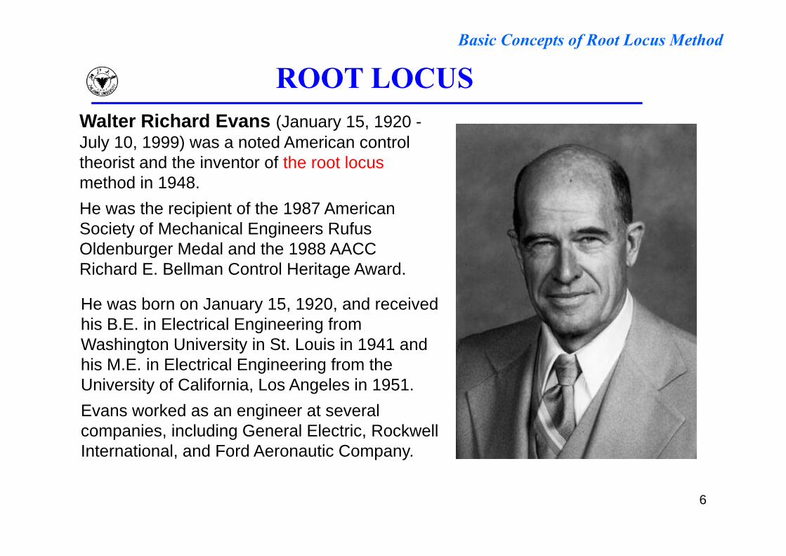
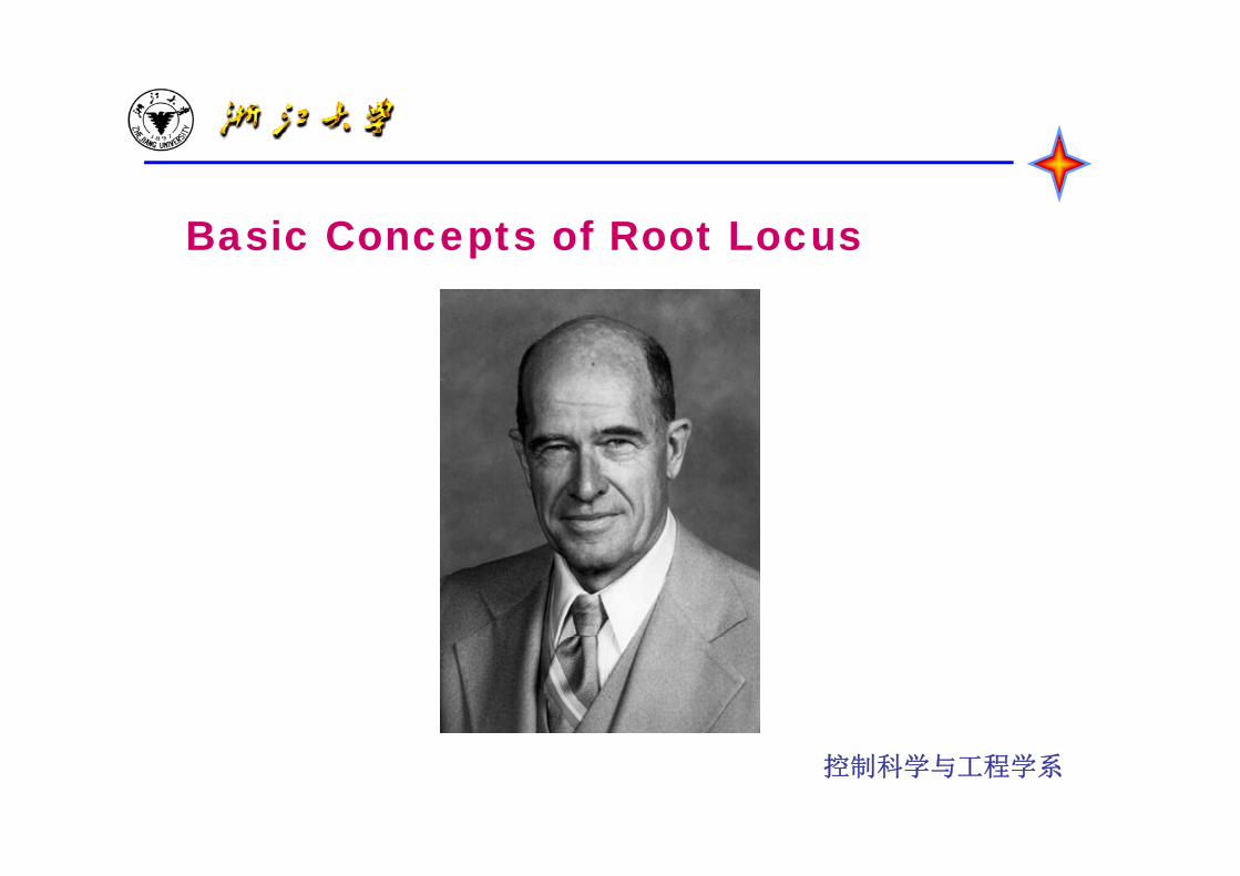
ROOT LOCUSWalter Richard Evans (January 15, 1920 -July 10, 1999) was a noted American control theorist and the inventor of the root locus method in 1948. He was the recipient of the 1987 American pSociety of Mechanical Engineers Rufus Oldenburger Medal and the 1988 AACC Richard E. Bellman Control Heritage Award.g
He was born on January 15, 1920, and received his B.E. in Electrical Engineering from Washington Uni ersit in St Lo is in 1941 andWashington University in St. Louis in 1941 and his M.E. in Electrical Engineering from the University of California, Los Angeles in 1951.E k d i lEvans worked as an engineer at several companies, including General Electric, Rockwell International, and Ford Aeronautic Company.
6
Basic Concepts of Root Locus Method
ROOT LOCUS1. Introduction
Definition:
The root locus is a plot of the roots of the characteristic pequation of the closed-loop system as a function of one system parameter varies, such as the gain of the open-loop transfer function.
It is a method that determines how the poles move around the S-plane as we change one control parameter.
This plot was introduced by Evans in 1948 and has been p ydeveloped and used extensively in control engineering.
7
Basic Concepts of Root Locus Method
ROOT LOCUS1. Introduction
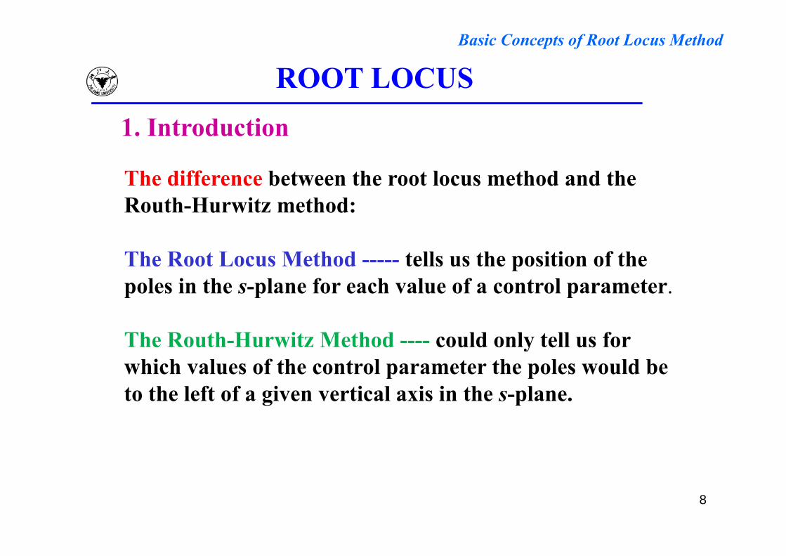
The difference between the root locus method and the Routh-Hurwitz method:
The Root Locus Method ----- tells us the position of the i f fpoles in the s-plane for each value of a control parameter.
The Routh-Hurwitz Method ---- could only tell us forThe Routh-Hurwitz Method ---- could only tell us for which values of the control parameter the poles would be to the left of a given vertical axis in the s-plane.g p
8
Basic Concepts of Root Locus Method
ROOT LOCUS1. Introduction
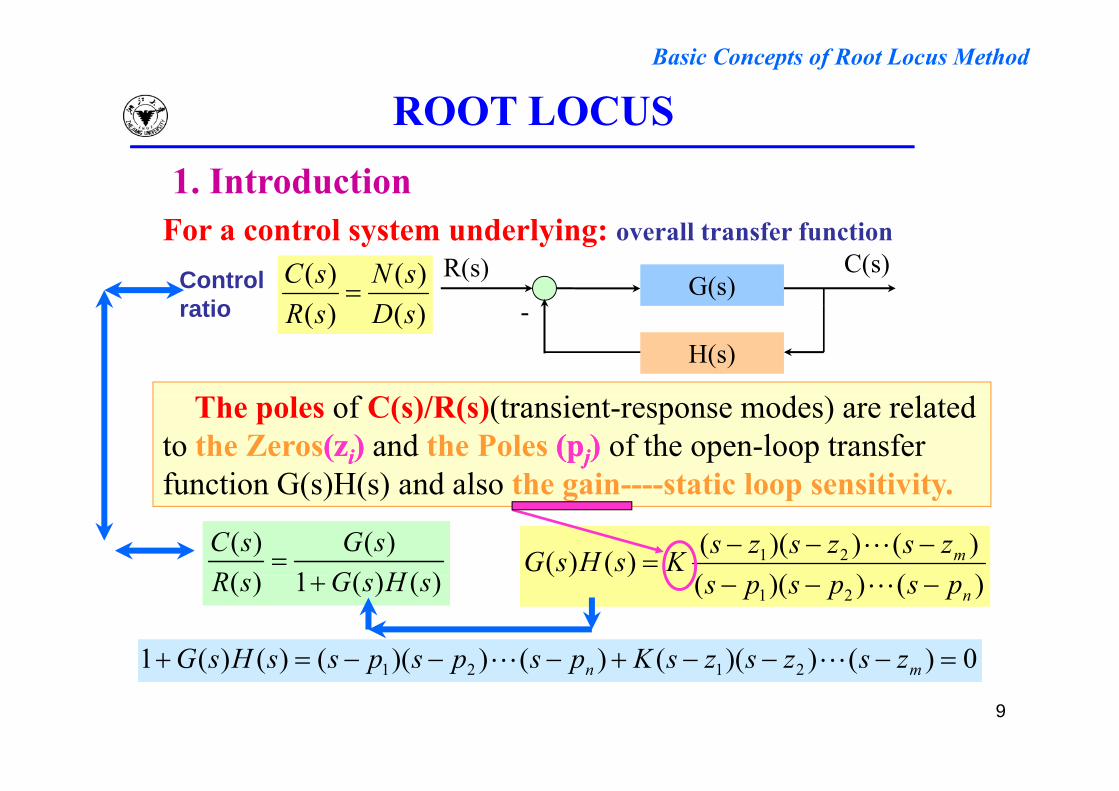
For a control system underlying: overall transfer function
G(s)R(s) C(s)
)()(
)()(
DsN
RsCControl
ratio
f ( i d ) l d
H(s)-)()( sDsRratio
The poles of C(s)/R(s)(transient-response modes) are related to the Zeros((zzii)) and the Poles ((ppjj)) of the open-loop transfer function G(s)H(s) and also the gain----static loop sensitivityfunction G(s)H(s) and also the gain----static loop sensitivity.
)())(()())(()()( 21 mzszszsKsHsG
)()(1)(
)()(
HGsG
RsC
)())((
)()(21 npspsps )()(1)( sHsGsR
0)())(()())(()()(1 2121 zszszsKpspspssHsG
9
0)())(()())(()()(1 2121 mn zszszsKpspspssHsG
Basic Concepts of Root Locus Method
ROOT LOCUS1. Introduction
The advantage of the root locus method:
Th t f th h t i ti ti f th t b• The roots of the characteristic equation of the system can be obtained directly.
i i f• The characteristic of the system can be completely and accurately yielded.
• Design a system with relative ease. Such as using MATLAB.
10
Basic Concepts of Root LocusBasic Concepts of Root Locus
控制科学与工程学系
Basic Concepts of Root Locus Method
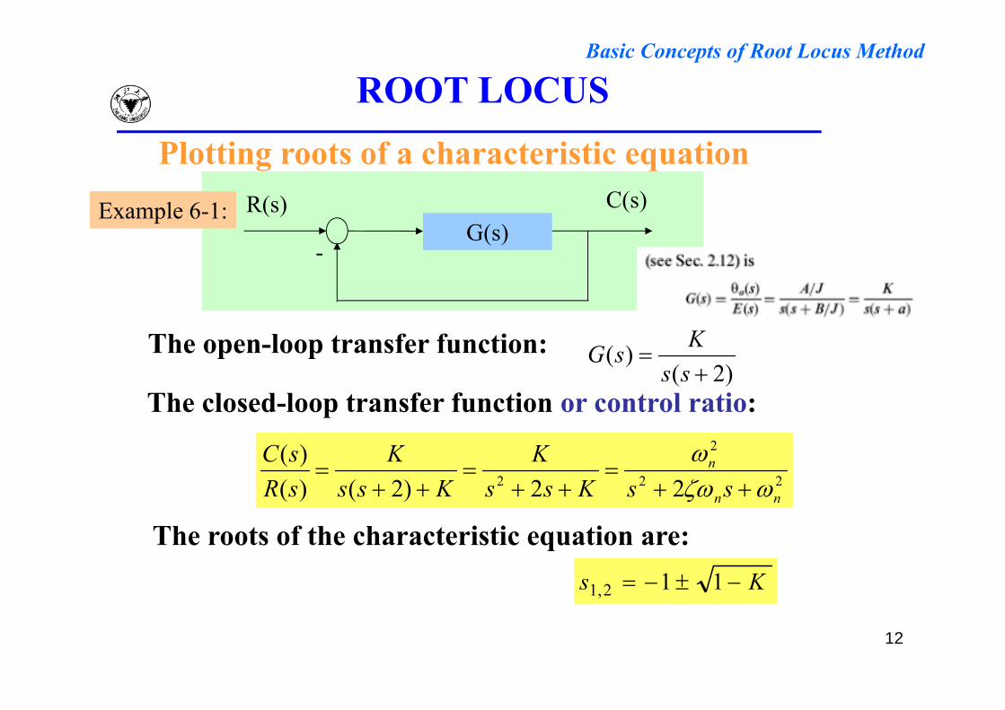
ROOT LOCUSPlotting roots of a characteristic equation
C( )G(s)
-
R(s) C(s)Example 6-1:
)( KsGThe open-loop transfer function:
)2()(
sssGp p
The closed-loop transfer function or control ratio:
22
2
2 22)2()()(
nn
n
ssKssK
KssK
sRsC
Ks 112,1
The roots of the characteristic equation are:
12
,
Basic Concepts of Root Locus Method
ROOT LOCUS Gain of the open-loop transfer function
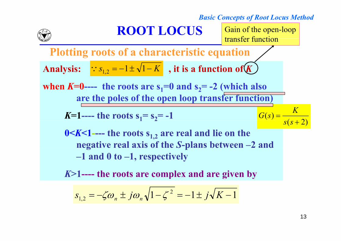
A l i i i f i f KK 11
Plotting roots of a characteristic equationtransfer function
Analysis: , it is a function of K
when K=0---- the roots are s1=0 and s2= -2 (which also
Ks 112,1
are the poles of the open loop transfer function)
K=1---- the roots s1= s2= -1)2(
)(
KsG1 2
0<K<1---- the roots s1,2 are real and lie on the negative real axis of the S-plans between –2 and
)2( ss
eg ve e s o e S p s be wee d–1 and 0 to –1, respectively
K>1---- the roots are complex and are given by
111 22,1 Kjjs nn
K>1 the roots are complex and are given by
13
Basic Concepts of Root Locus Method
ROOT LOCUS)2(
)( KsG
Plotting roots of a characteristic equation )2(
)(ss
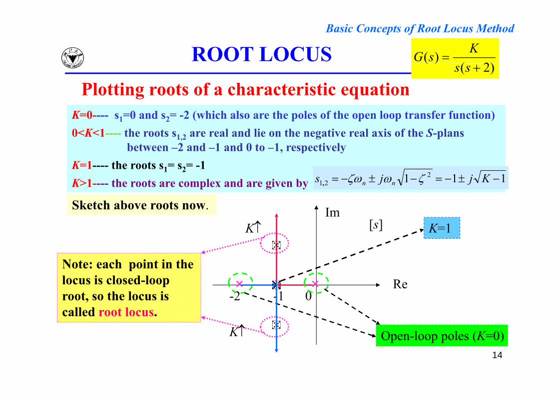
K=0---- s1=0 and s2= -2 (which also are the poles of the open loop transfer function)0<K<1---- the roots s1,2 are real and lie on the negative real axis of the S-plans
between –2 and –1 and 0 to –1, respectively, p yK=1---- the roots s1= s2= -1K>1---- the roots are complex and are given by 111 2
21 Kjjs nn ,
Im[s]
Sketch above roots now.
K=1K
ReNote: each point in the locus is closed-loop Re
-2 0-1
O l l (K 0)
root, so the locus is called root locus.
K
14
Open-loop poles (K=0)K
Basic Concepts of Root Locus Method
ROOT LOCUS )( KsG
’ i f i i f
Plotting roots of a characteristic equation)2(
)(ss
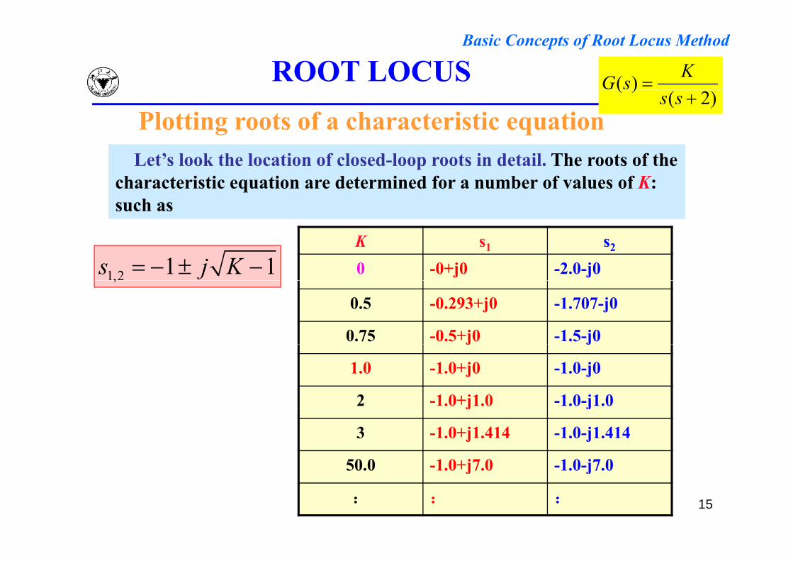
Let’s look the location of closed-loop roots in detail. The roots of the characteristic equation are determined for a number of values of K: such as
K s1 s2
0 -0+j0 -2.0-j01,2 1 1s j K 0.5 -0.293+j0 -1.707-j0
0.75 -0.5+j0 -1.5-j0
,
j j
1.0 -1.0+j0 -1.0-j0
2 -1.0+j1.0 -1.0-j1.0j j
3 -1.0+j1.414 -1.0-j1.414
50.0 -1.0+j7.0 -1.0-j7.0
15
j j
: : :
Basic Concepts of Root Locus Method
ROOT LOCUS )( KsG
Plotting roots of a characteristic equation)2(
)(ss
sG
j2.0jω
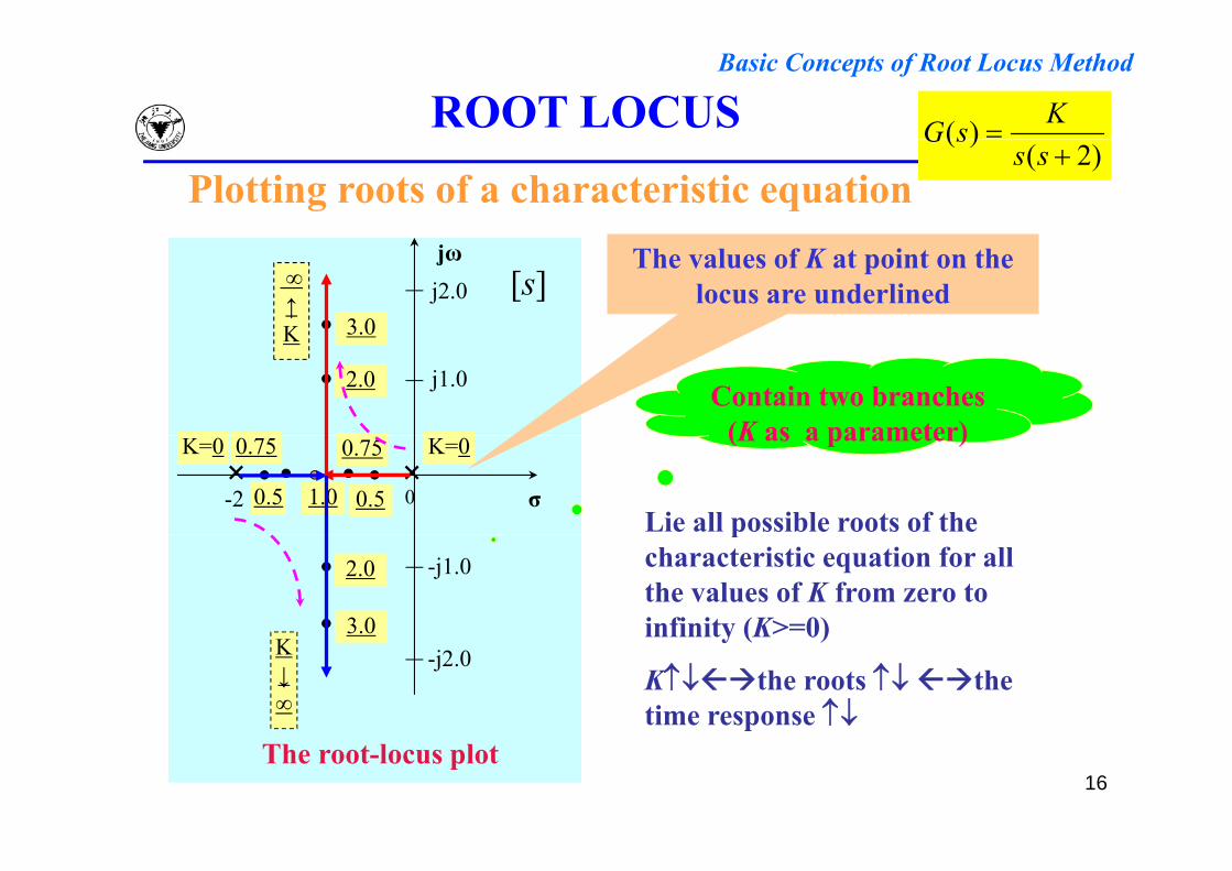
[s]The values of K at point on the
locus are underlined3.0
∞↑K
j1.02.0
K
Contain two branches(K as a parameter)
-2 0 σ-1
K=0K=0
0.50.5
0.750.75
1.0Lie all possible roots of the
(K as a parameter)
-j1.02.0
3.0
pcharacteristic equation for all the values of K from zero to infinity (K>=0)
-j2.03.0
K↓∞
infinity (K> 0)
Kthe roots the time response
16The root-locus plot
Basic Concepts of Root Locus Method
ROOT LOCUSPlotting roots of a characteristic equation
G(s)-
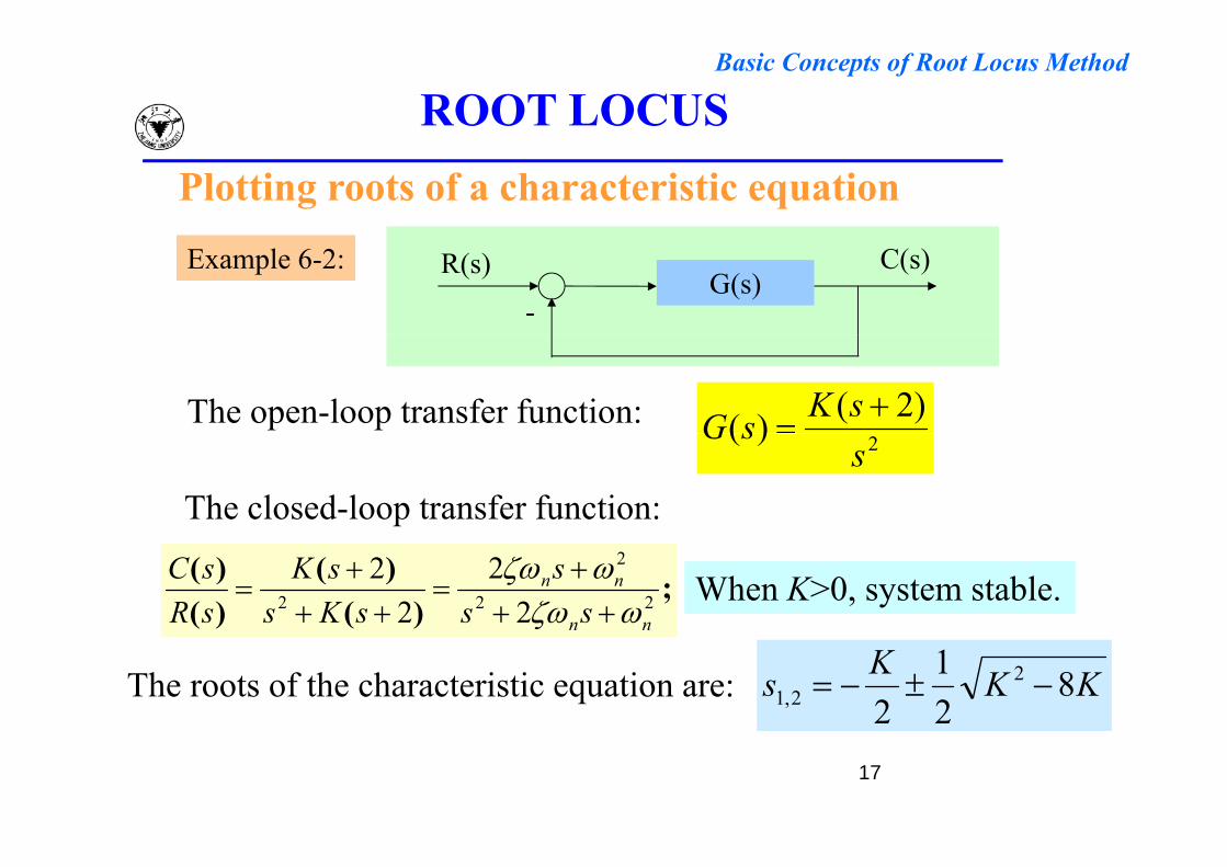
R(s) C(s)Example 6-2:
)2()( sKsG The open-loop transfer function:
2)(s
sG
The closed-loop transfer function:
;)(
)()()(
22
2
2 22
22
nn
nn
sss
sKssK
sRsC
When K>0, system stable.
KKKs 821
22
2,1 The roots of the characteristic equation are:
17
Basic Concepts of Root Locus Method
ROOT LOCUSPlotting roots of a characteristic equation
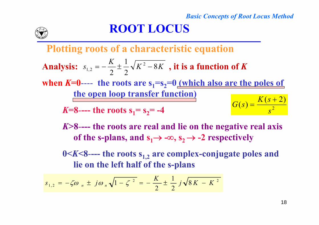
K 1Analysis: , it is a function of K
when K=0---- the roots are s1=s2=0 (which also are the poles of
KKKs 821
22
2,1
1 2 ( pthe open loop transfer function)
K=8---- the roots s1= s2= -4 2
)2()(ssKsG
K 8 the roots s1 s2 4
K>8---- the roots are real and lie on the negative real axis of the s-plans and s - s -2 respectively
s
of the s-plans, and s1 -, s2 -2 respectively
0<K<8---- the roots s1,2 are complex-conjugate poles and lie on the left half of the s plans
222,1 8
21
21 KKjKjs nn
lie on the left half of the s-plans
18
22
Basic Concepts of Root Locus Method
ROOT LOCUS KKKs 821
22
2,1 2
)2()(ssKsGopen
Plotting roots of a characteristic equation222,1s
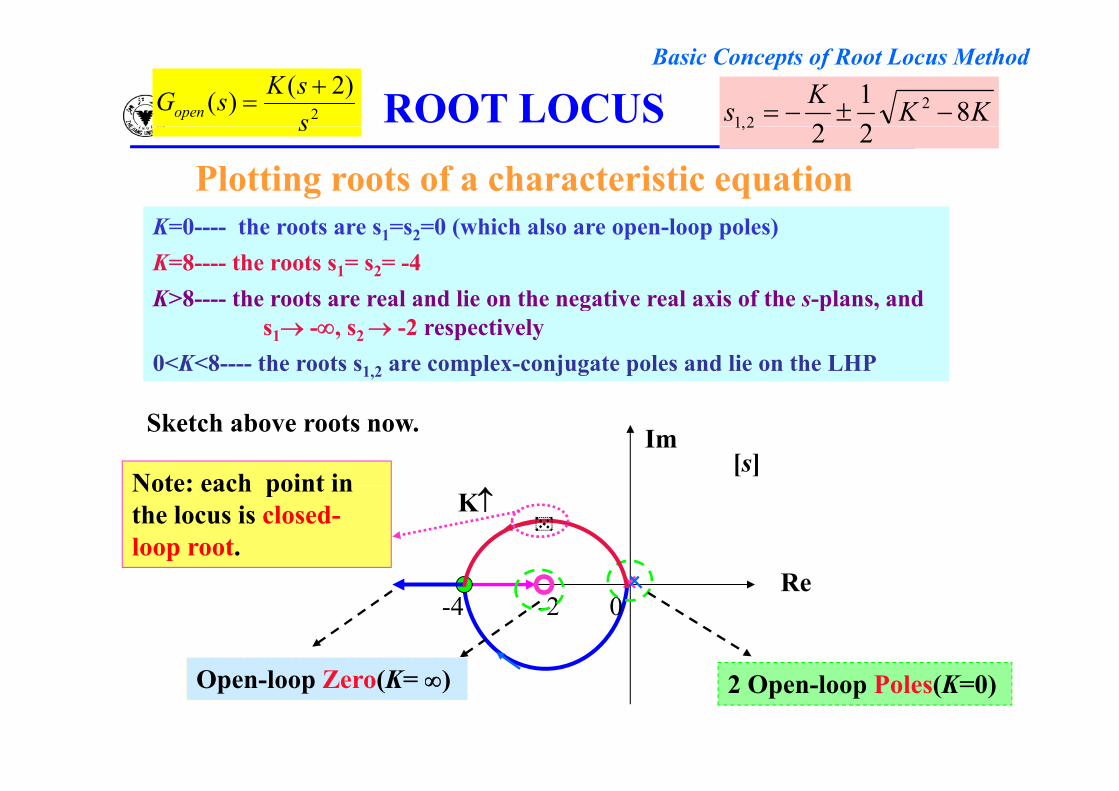
K=0---- the roots are s1=s2=0 (which also are open-loop poles)K=8---- the roots s1= s2= -4K>8---- the roots are real and lie on the negative real axis of the s-plans, andK 8 the roots are real and lie on the negative real axis of the s plans, and
s1 -, s2 -2 respectively0<K<8---- the roots s1,2 are complex-conjugate poles and lie on the LHP
Im[s]
Note: each point in
Sketch above roots now.
R
KNote: each point in the locus is closed-loop root.
Re-2 0-4
2 Open-loop Poles(K=0)Open-loop Zero(K= )
Basic Concepts of Root Locus Method
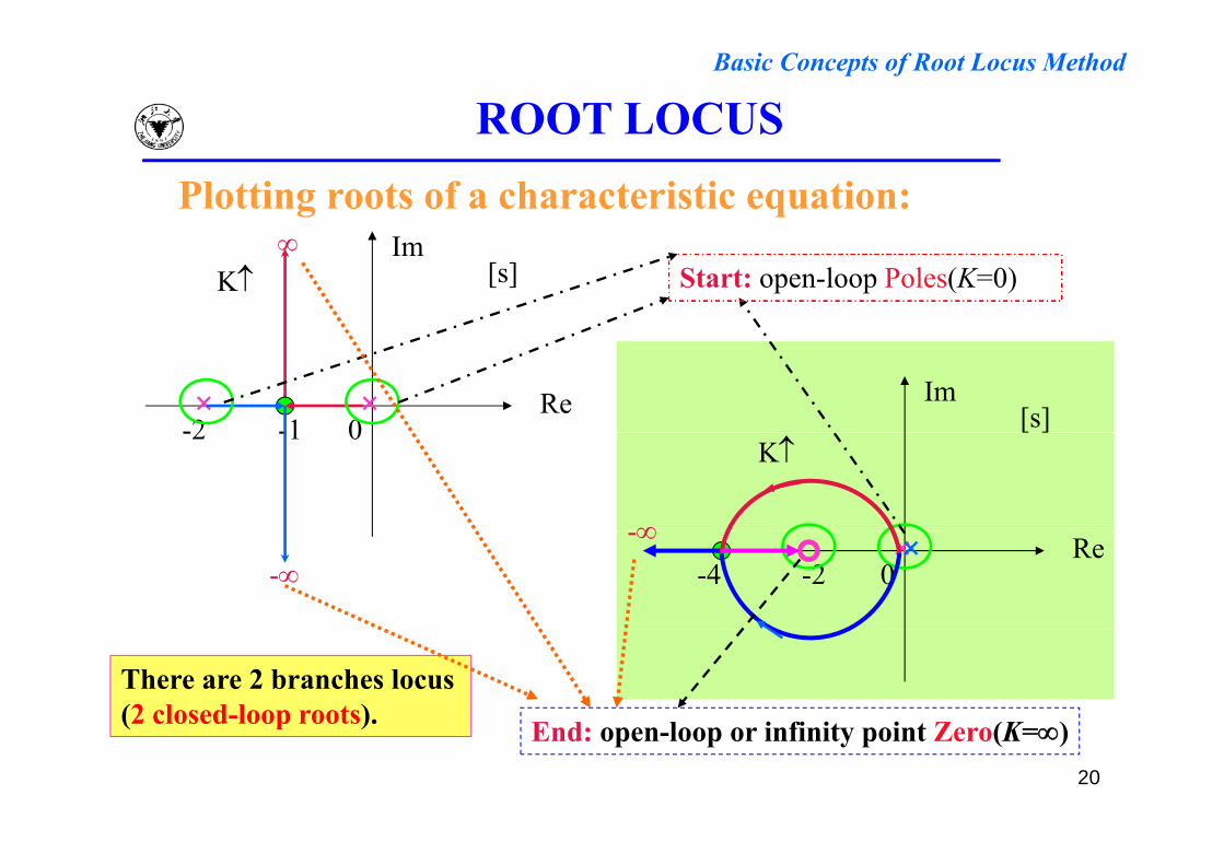
ROOT LOCUSPlotting roots of a characteristic equation:
Im[s]K
Start: open-loop Poles(K=0)
Im[s]Re
-2 0-1 [ ]K
-2 0-1
Re-2 0-4
--
There are 2 branches locus (2 closed-loop roots). E d l i fi it i t Z (K )
20
( p ) End: open-loop or infinity point Zero(K=)
Basic Concepts of Root Locus Method
ROOT LOCUSPlotting roots of a characteristic equation
G(s)-
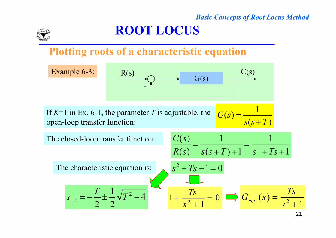
R(s) C(s)Example 6-3:
)(1)(T
sG If K=1 in Ex. 6-1, the parameter T is adjustable, the l f f i )(
)(Tss open-loop transfer function:
11)(
sCThe closed-loop transfer function:
11)()( 2 TssTsssR
The characteristic equation is: 012 Tss
01 2 Ts )( 2
TssGeqo41 221 TTs
21
01
1 2 s 1
)( 2 sGeqo222,1
Basic Concepts of Root Locus Method
ROOT LOCUS Plotting roots of a characteristic equation
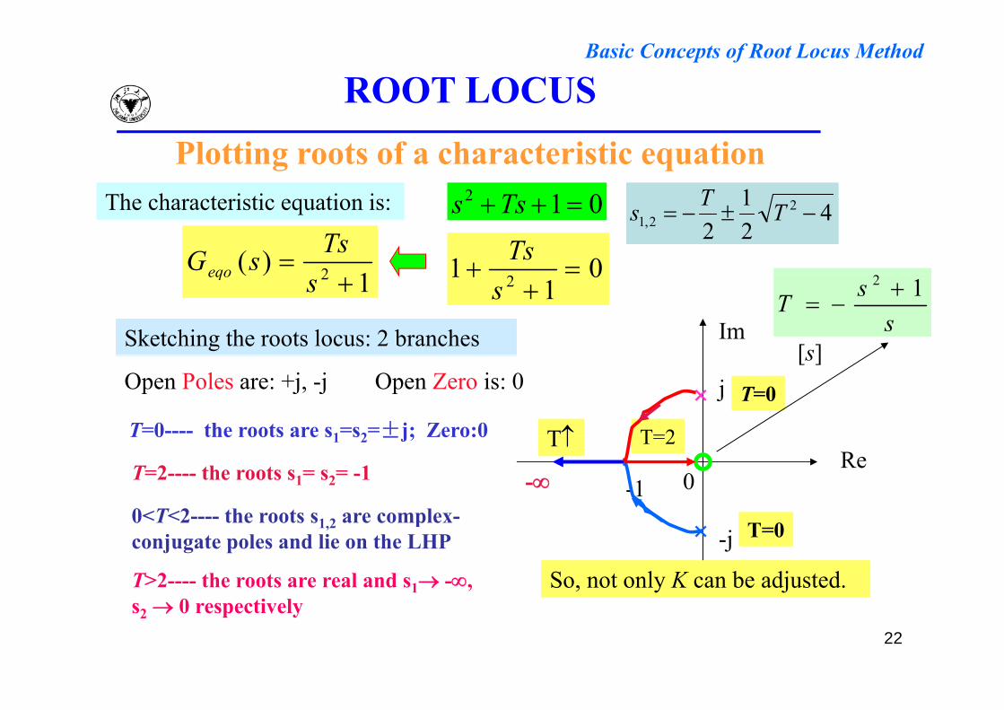
h h i i i i 2 1TThe characteristic equation is: 012 Tss
01 Ts
1)( 2
TssGeqo
421
22
2,1 TTs
Im[s]
01
1 2 s1
)( 2 seqo
Sketching the roots locus: 2 branches ssT 12
[s]
T=2T
j T=0Open Poles are: +j, -j Open Zero is: 0
T=0---- the roots are s1=s2=±j; Zero:0Re
T=2
-1
T
- 0
T 0 the roots are s1 s2 ±j; Zero:0
T=2---- the roots s1= s2= -1
0<T<2 the roots s are complex-j T=0
So, not only K can be adjusted.
0<T<2---- the roots s1,2 are complex-conjugate poles and lie on the LHP
T>2---- the roots are real and s1 -,
22
s2 0 respectively
Basic Concepts of Root Locus Method
ROOT LOCUSPlotting roots of a characteristic equation
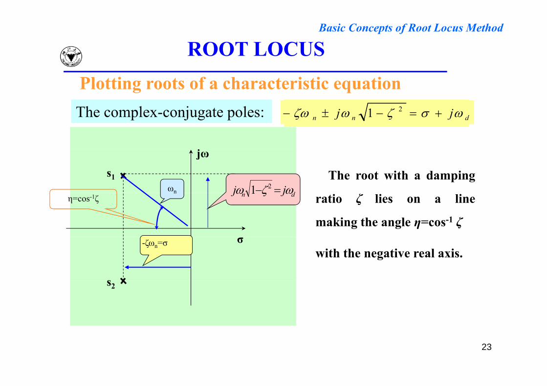
j
The complex-conjugate poles: dnn jj 21
jω
The root with a dampings1
djj 21ωnratio ζ lies on a line
making the angle η=cos-1 ζ
dn jj 1nη=cos-1ζ
σwith the negative real axis.
s
-ζωn=σ
s2
23
Basic Concepts of Root Locus Method
ROOT LOCUS
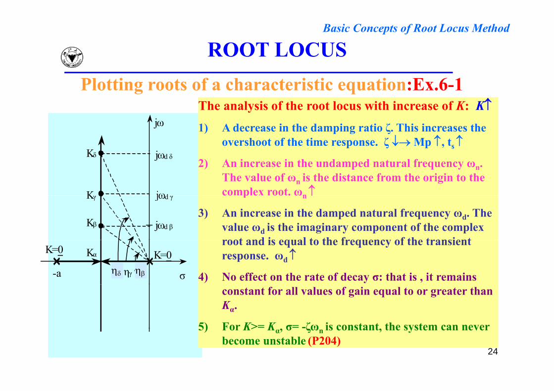
The analysis of the root locus with increase of K: KPlotting roots of a characteristic equation:Ex.6-1
The analysis of the root locus with increase of K: K
1) A decrease in the damping ratio ζ. This increases the overshoot of the time response. ζ Mp , ts
jω
jK2) An increase in the undamped natural frequency ωn.
The value of ωn is the distance from the origin to the complex root. ωnjωd
jωd δ
K
Kδ
co p e oo . ωn
3) An increase in the damped natural frequency ωd. The value ωd is the imaginary component of the complex root and is equal to the frequency of the transient
jωd β
jωd γ
Kβ
Kγ
root and is equal to the frequency of the transient response. ωd
4) No effect on the rate of decay σ: that is , it remains -a σηβ ηγ ηδ
K=0 K=0Kα
constant for all values of gain equal to or greater than Kα.
5) For K>= K , σ= -ζω is constant, the system can never
24
5) For K> Kα, σ ζωn is constant, the system can never become unstable (P204)
Basic Concepts of Root Locus Method
ROOT LOCUSQualitative analysis of the root locus
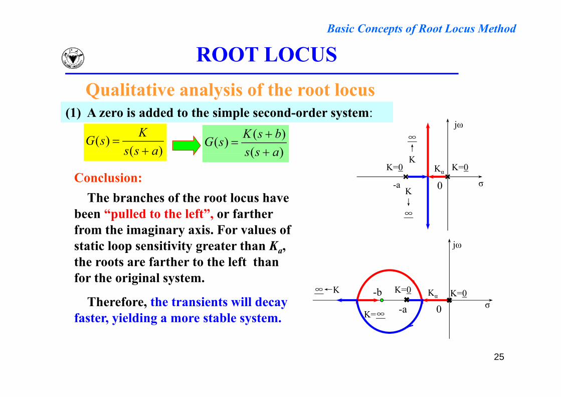
(1) A i dd d h i l d d(1) A zero is added to the simple second-order system:
)()(
assKsG
)()()(assbsKsG
jω
∞↑
Conclusion:The branches of the root locus have
)( ass )( ass
-a σ
K=0 K=0Kα
K
K↓
0The branches of the root locus have
been “pulled to the left”, or farther from the imaginary axis. For values of t ti l iti it t th K jω
↓∞
static loop sensitivity greater than Ka, the roots are farther to the left than for the original system.
K=0∞←K
jω
bTherefore, the transients will decay
faster, yielding a more stable system.-a
K=0 K=0Kα∞←K
K=∞σ
-b0
25
Basic Concepts of Root Locus Method
ROOT LOCUSQualitative analysis of the root locus
jω
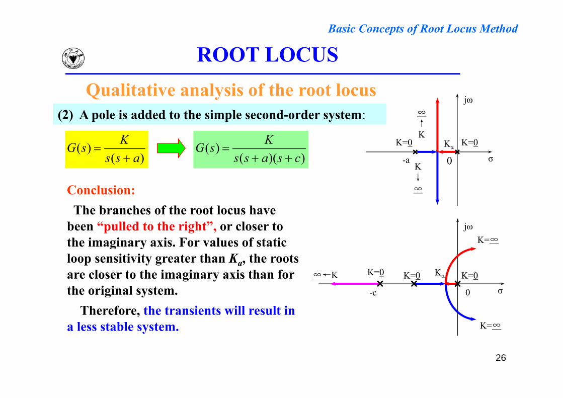
(2) A pole is added to the simple second-order system:
)()( KsG
))(()( KsG K=0 K=0Kα
∞↑K
Conclusion:
)()(
ass ))(()(
csass -a σK↓∞
0
The branches of the root locus have been “pulled to the right”, or closer to the imaginary axis For values of static
jωK=∞the imaginary axis. For values of static
loop sensitivity greater than Ka, the roots are closer to the imaginary axis than for the original system 0 σ
K=0 K=0Kα∞←K K=0
the original system.Therefore, the transients will result in
a less stable system.
0 σ-c
K=∞
26
Basic Concepts of Root Locus Method
ROOT LOCUSQualitative analysis of the root locus
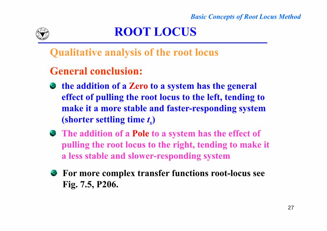
General conclusion:the addition of a Zero to a system has the general y geffect of pulling the root locus to the left, tending to make it a more stable and faster-responding system (shorter settling time ts)The addition of a Pole to a system has the effect of
lli th t l t th i ht t di t k itpulling the root locus to the right, tending to make it a less stable and slower-responding system
For more complex transfer functions root-locus see Fig. 7.5, P206.
27
Basic Concepts of Root Locus Method
ROOT LOCUSProcedure outline of plotting root locus
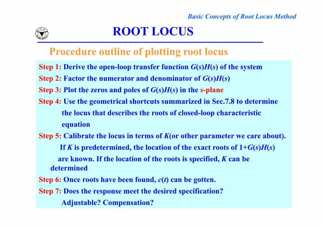
Step 1: Derive the open-loop transfer function G(s)H(s) of the systemStep 2: Factor the numerator and denominator of G(s)H(s) St 3 Pl t th d l f G( )H( ) i th lStep 3: Plot the zeros and poles of G(s)H(s) in the s-planeStep 4: Use the geometrical shortcuts summarized in Sec.7.8 to determine
the locus that describes the roots of closed-loop characteristicthe locus that describes the roots of closed loop characteristic equation
Step 5: Calibrate the locus in terms of K(or other parameter we care about).If K is predetermined, the location of the exact roots of 1+G(s)H(s)
are known. If the location of the roots is specified, K can be d t i ddetermined
Step 6: Once roots have been found, c(t) can be gotten.Step 7: Does the response meet the desired specification?
28
Step 7: Does the response meet the desired specification?Adjustable? Compensation?
Basic Concepts of Root Locus Method
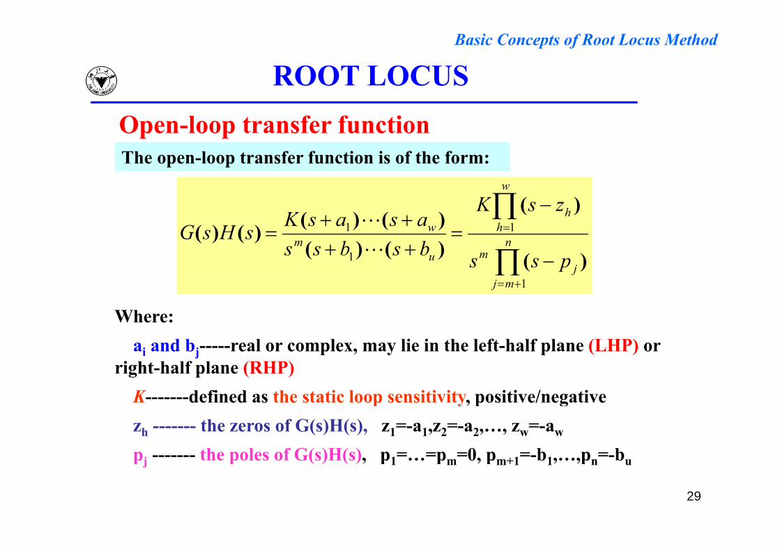
ROOT LOCUSOpen-loop transfer functionThe open-loop transfer function is of the form:
w
hzsKK
)()()(
n
jm
hh
um
w
pssbsbssasasKsHsG 1
1
1
)(
)(
)()()()()()(
mj 1
Where: i i f f ( )ai and bj-----real or complex, may lie in the left-half plane (LHP) or
right-half plane (RHP)K-------defined as the static loop sensitivity, positive/negativeK defined as the static loop sensitivity, positive/negativezh ------- the zeros of G(s)H(s), z1=-a1,z2=-a2,…, zw=-aw
pj ------- the poles of G(s)H(s), p1=…=pm=0, pm+1=-b1,…,pn=-bu
29
pj p ( ) ( ) p1 pm pm+1 1 pn u
Basic Concepts of Root Locus Method
ROOT LOCUSPoles of Closed-loop transfer function
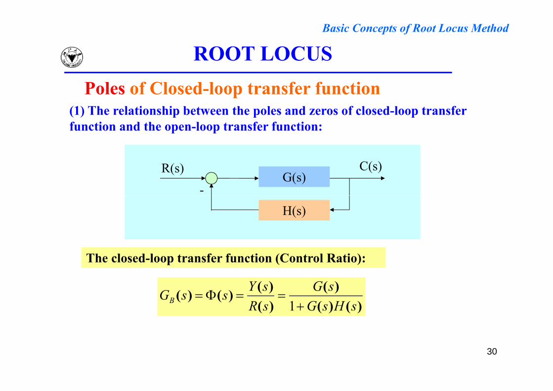
(1) Th l ti hi b t th l d f l d l t f(1) The relationship between the poles and zeros of closed-loop transfer function and the open-loop transfer function:
G(s)-
R(s) C(s)
H(s)
The closed-loop transfer function (Control Ratio):
)()( GY)()(
)()()()()(
sHsGsG
sRsYssGB
1
30
Basic Concepts of Root Locus Method
ROOT LOCUSPoles of Closed-loop transfer function
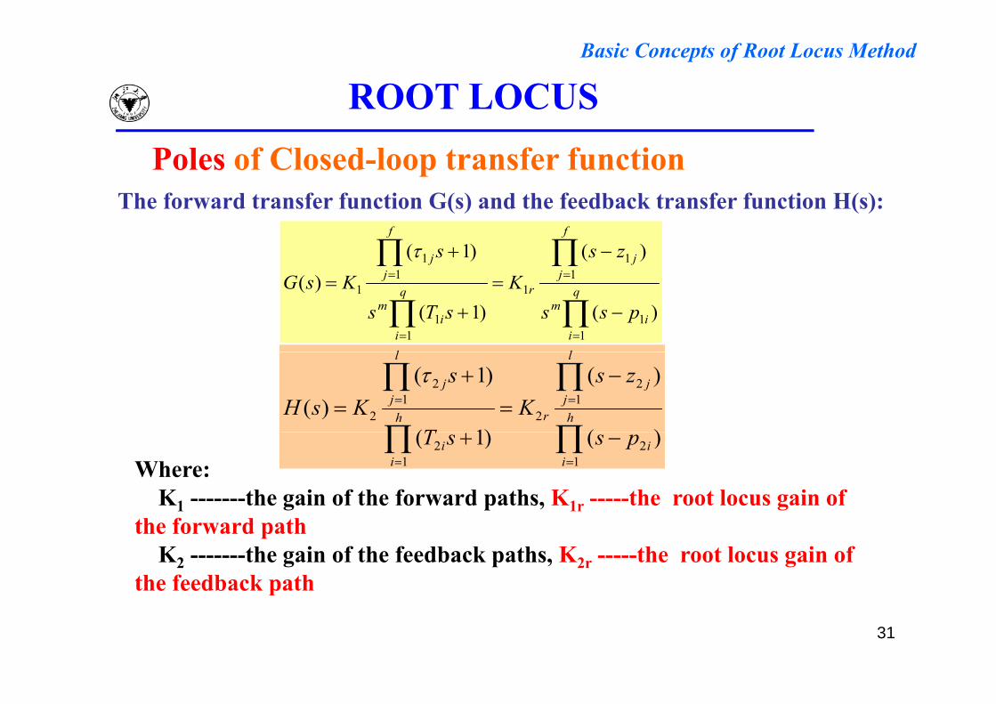
The forward transfer function G(s) and the feedback transfer function H(s):
f
jj
f
jj zss
11
11 )()1(
q
ii
m
jrq
ii
m
j
pssK
sTsKsG
11
11
11
11
)()1()(
ll
h
l
jj
rh
l
jj zs
KT
sKsH 1
2
21
2
2
)(
)(
)1(
)1()(
Where:K1 -------the gain of the forward paths, K1r -----the root locus gain of
i
ii
i pssT1
21
2 )()1(
the forward path K2 -------the gain of the feedback paths, K2r -----the root locus gain of
the feedback path
31
p
Basic Concepts of Root Locus Method
ROOT LOCUSPoles of Closed-loop transfer function
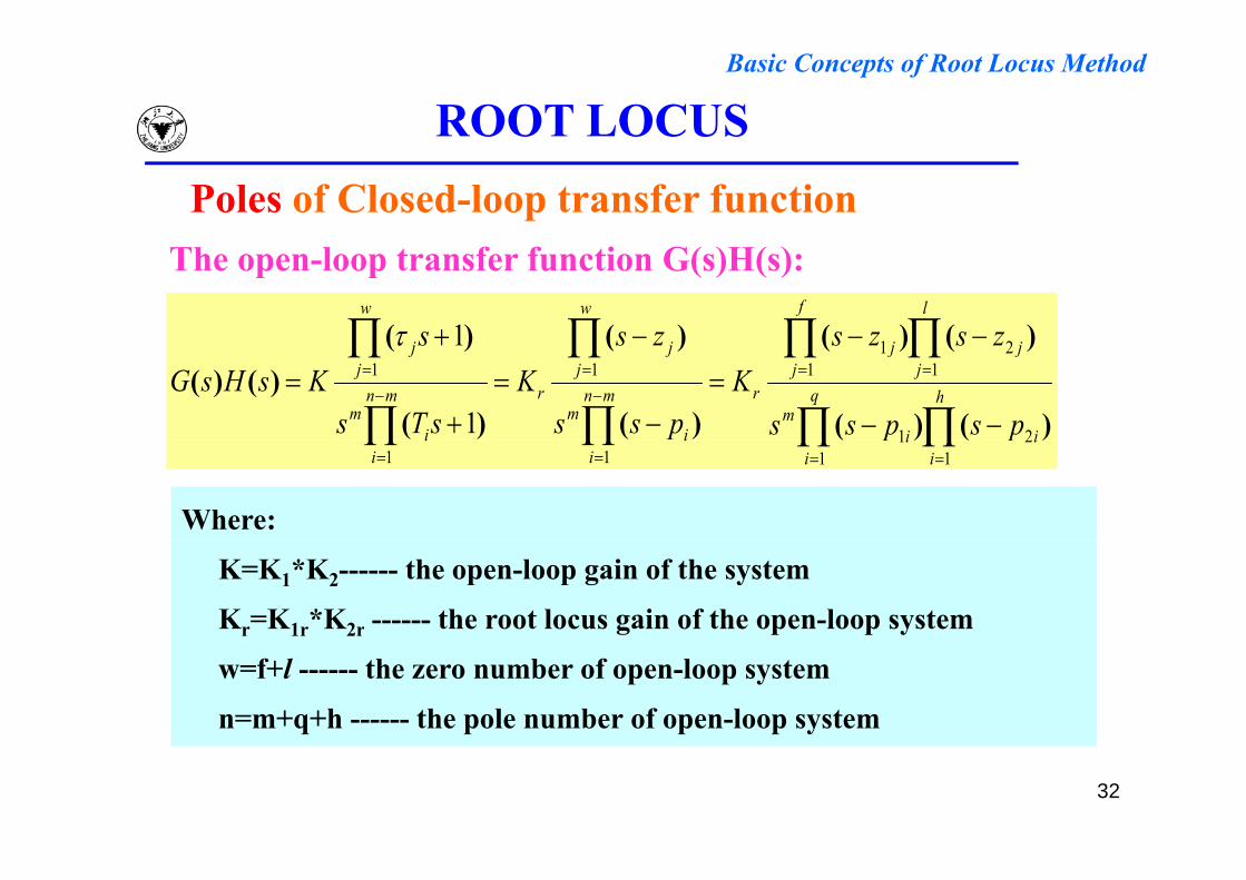
The open-loop transfer function G(s)H(s):
lfww
zszszss 1 )()()()(
h
i
q
im
jj
jj
rmn
im
jj
rmn
im
jj
pspss
zszsK
pss
zsK
sTs
sKsHsG
21
12
11
11
1
1
)()(
)()(
)(
)(
)(
)()()(
i
ii
ii
ii
i pp1
21
111
)()(
Where:
K=K1*K2------ the open-loop gain of the system
Kr=K1r*K2r ------ the root locus gain of the open-loop system
w=f+l ------ the zero number of open-loop system
n=m+q+h ------ the pole number of open-loop system
32
Basic Concepts of Root Locus Method
ROOT LOCUS
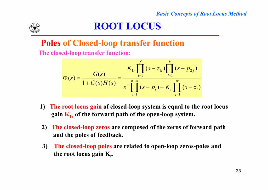
The closed loop transfer function:Poles of Closed-loop transfer function
h
j
f
ir pszsKsG
211 )()()(
The closed-loop transfer function:
w
jir
mn
ii
m
ji
zsKpsssHsG
sGs
11
11
)()()()(1
)()(
ji 11
1) The root locus gain of closed-loop system is equal to the root locus gain K1r of the forward path of the open-loop system. g 1r p p p y
2) The closed-loop zeros are composed of the zeros of forward path and the poles of feedback.p
3) The closed-loop poles are related to open-loop zeros-poles and the root locus gain Kr.
33
Basic Concepts of Root Locus Method
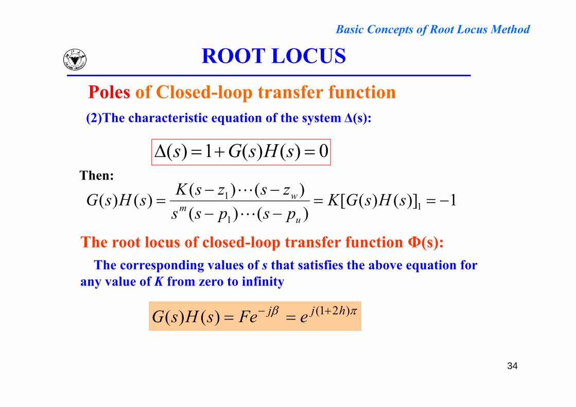
ROOT LOCUSPoles of Closed-loop transfer function(2)The characteristic equation of the system Δ(s):
0)()(1)( sHsGs )()()(
1)]()([)()()()( 11
sHsGKzszsKsHsG w
Then:
The root locus of closed-loop transfer function Φ(s):
1)]()([)()(
)()( 11
sHsGKpspss
sHsGu
m
p ( )The corresponding values of s that satisfies the above equation for
any value of K from zero to infinity
)21()()( hjj eFesHsG
34
Basic Concepts of Root Locus Method
ROOT LOCUS 1)]()([)()()()()()( 1
1
1
sHsGKpspsszszsKsHsGu
mw
Poles of Closed-loop transfer function
)()( 1 pp u
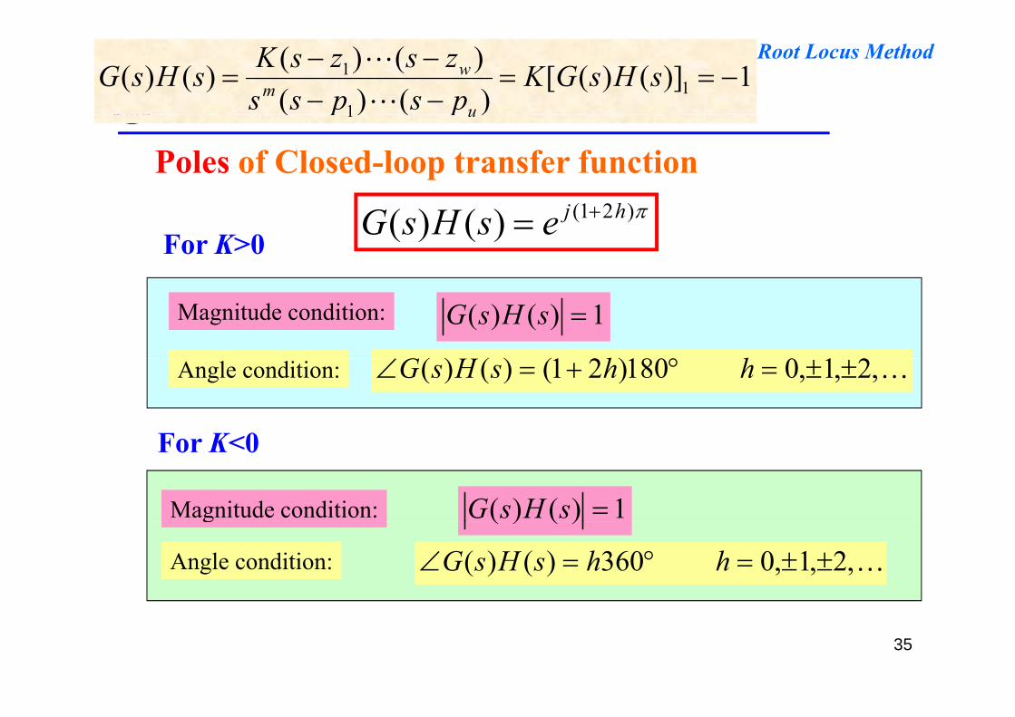
For K>0)21()()( hjesHsG
210180)21()()( hhG
1)()( sHsGMagnitude condition:
For K<0
,2,1,0180)21()()( hhsHsGAngle condition:
For K<0
1)()( sHsGMagnitude condition: )()(
,2,1,0360)()( hhsHsGAngle condition:
g
35
Basic Concepts of Root Locus Method
ROOT LOCUS
E l 6 4Poles of Closed-loop transfer function
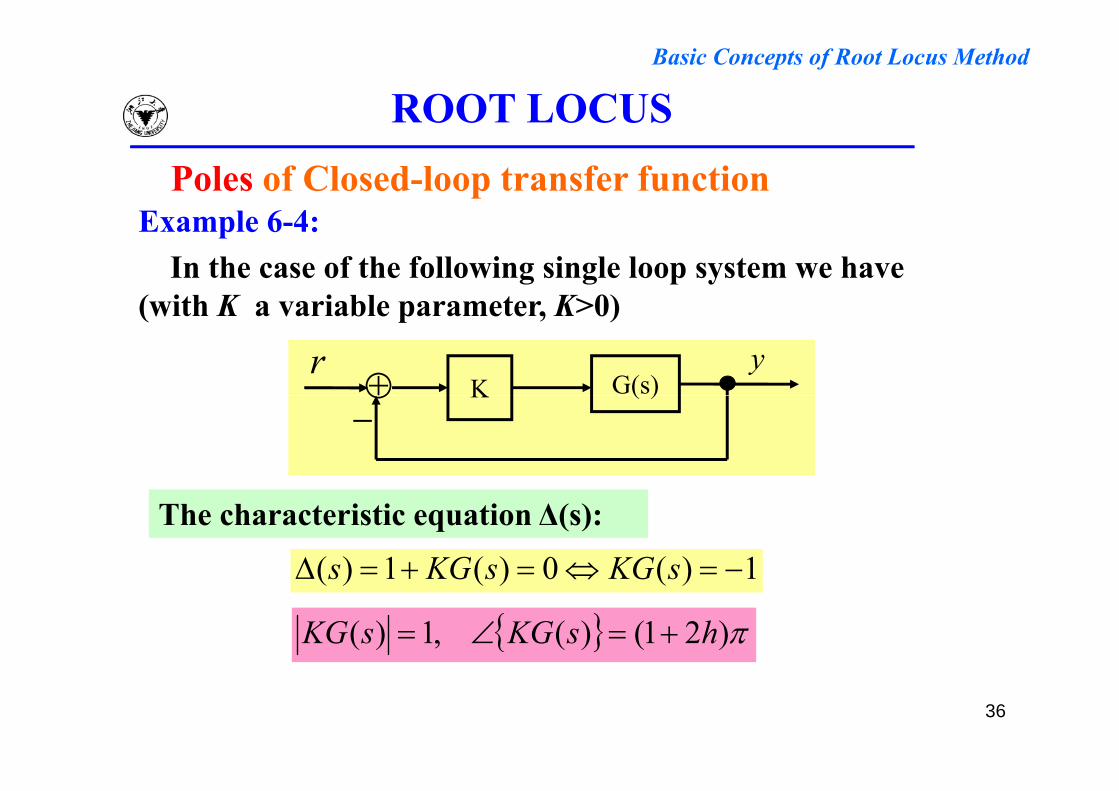
Example 6-4:In the case of the following single loop system we have
(with K a variable parameter K>0)(with K a variable parameter, K>0)
G(s)r y
K ( )_ K
1)(0)(1)( sKGsKGs
The characteristic equation Δ(s):
1)(0)(1)( sKGsKGs
)21()(,1)( hsKGsKG
36
Basic Concepts of Root Locus Method
ROOT LOCUSPoles of Closed-loop transfer function: Conclusion
The only possible locations for the poles in the s-plane are the ones that verify the angle condition above. K is then obtained from the magnitude condition.
From s(angle)K(magnitude)g g
All that needs to be done then is to identify the locations i th l th t lid l ti f th l fin the s-plane that are valid locations for the poles for a given value of the parameter K.
From given K s location
37
Basic Concepts of Root Locus Method
ROOT LOCUSApplication of the magnitude and angle conditions
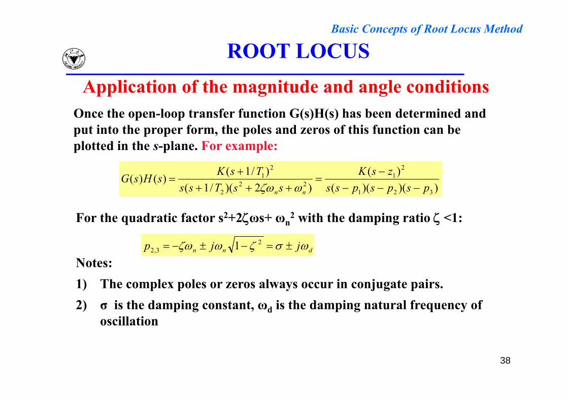
O th l t f f ti G( )H( ) h b d t i d dOnce the open-loop transfer function G(s)H(s) has been determined and put into the proper form, the poles and zeros of this function can be plotted in the s-plane. For example:
))()(()(
)2)(/1()/1()()(
321
21
222
21
pspspsszsK
ssTssTsKsHsG
nn
For the quadratic factor s2+2ωs+ ωn2 with the damping ratio <1:
jjp 21 dnn jjp 3,2 1Notes:1) The complex poles or zeros always occur in conjugate pairs.2) σ is the damping constant, ωd is the damping natural frequency of
oscillation
38
Basic Concepts of Root Locus Method
ROOT LOCUSApplication of the magnitude and angle conditions
jω
p2=σ+jωd s-z1
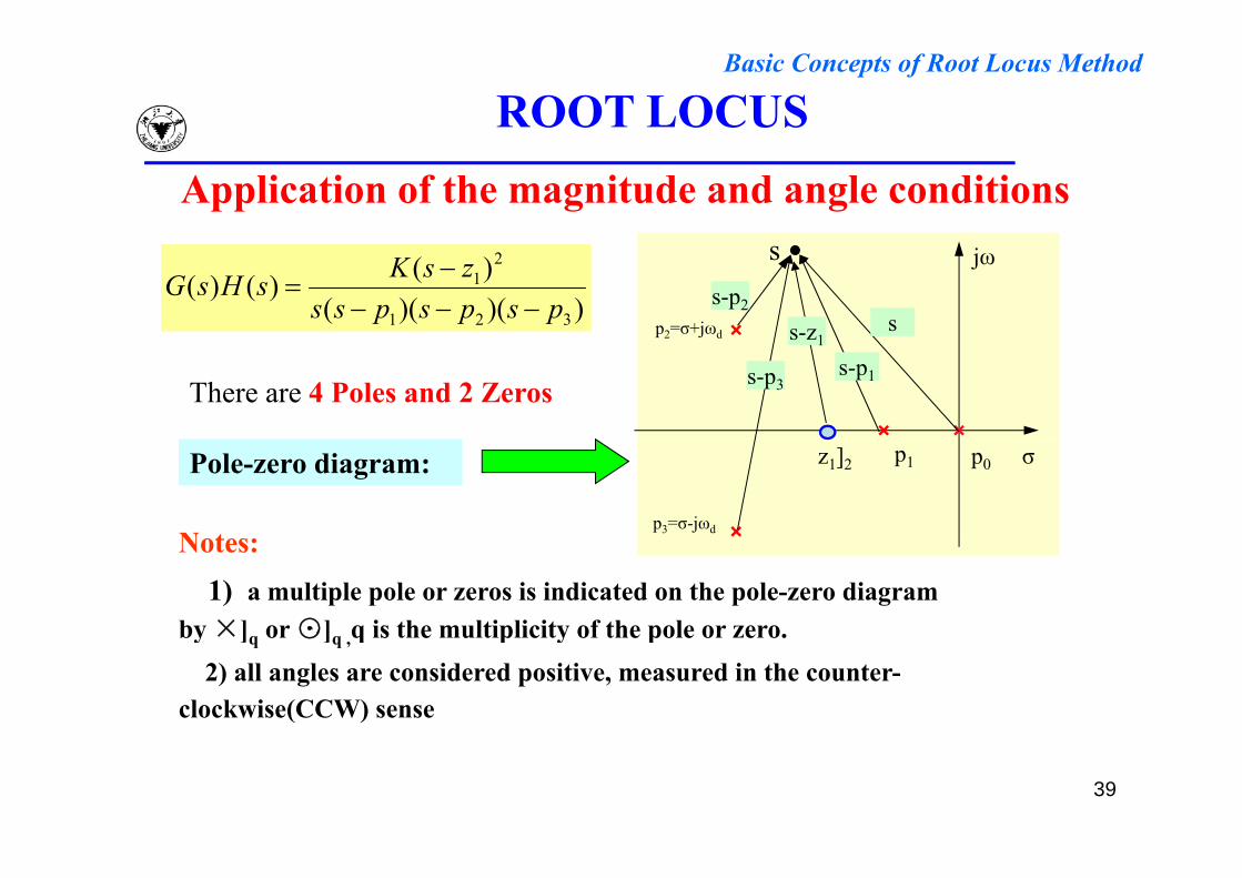
s-p2s))()((
)()()(321
21
pspspsszsKsHsG
s
s-p1
s z1
s-p3There are 4 Poles and 2 Zeros
σz1]2 p0
p3=σ-jωd
p1
Notes:
Pole-zero diagram:
Notes:1) a multiple pole or zeros is indicated on the pole-zero diagram
by ×]q or ⊙]q q is the multiplicity of the pole or zero.y ]q ⊙]q ,q p y p2) all angles are considered positive, measured in the counter-
clockwise(CCW) sense
39
Basic Concepts of Root Locus Method
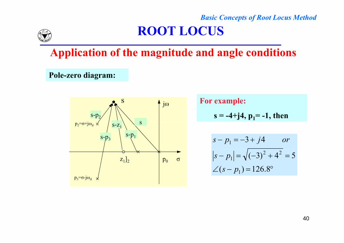
ROOT LOCUSApplication of the magnitude and angle conditions
Pole-zero diagram:
s-p2s
jω For example:
s = -4+j4, p1= -1, then
s
s-p1
s-z1
s-p3
sp2=σ+jωd
431 orjps
z1]2 p0
j
σ
8.126)(54)3(
1
221
psps
p3=σ-jωd
40
Basic Concepts of Root Locus Method
ROOT LOCUS
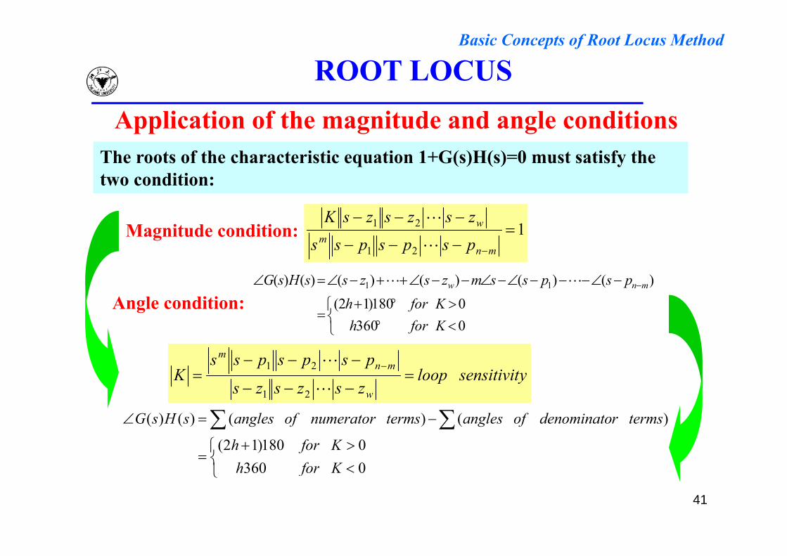
Th t f th h t i ti ti 1+G( )H( ) 0 t ti f th
Application of the magnitude and angle conditionsThe roots of the characteristic equation 1+G(s)H(s)=0 must satisfy the two condition:
zszszsK1
21
21
mnm
w
pspspss
zszszsK
Magnitude condition:
)()()()()()( HG
03600180)12(
)()()()()()( 11
KforhKforh
pspssmzszssHsG mnw Angle condition:
ysensitivitloopzszszs
pspspssK
w
mnm
21
21
03600180)12(
)()()()(
KforhKforh
termsrdenominatoofanglestermsnumeratorofanglessHsG
41
0360 Kforh
Basic Concepts of Root Locus Method
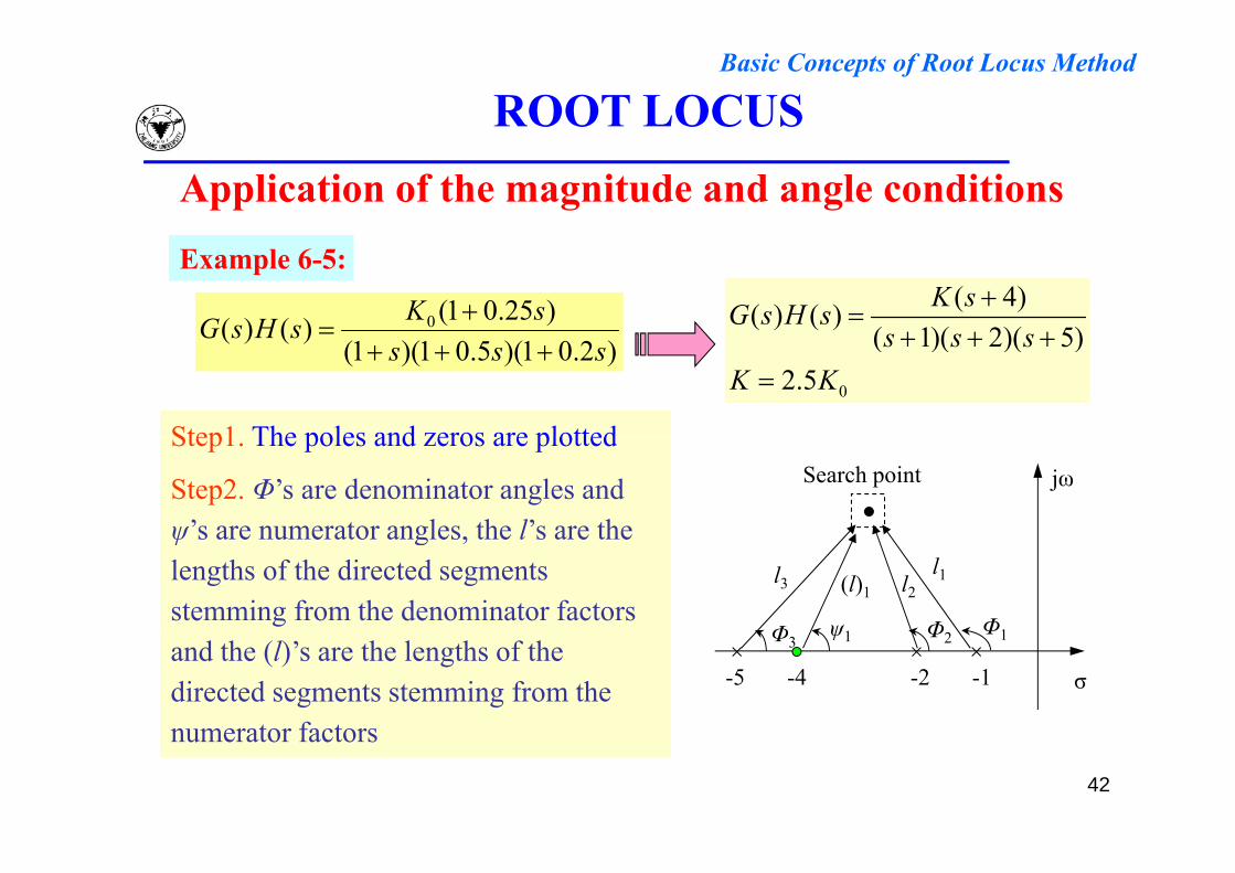
ROOT LOCUSApplication of the magnitude and angle conditionsExample 6-5:
)25.01()()( 0 sKsHsG
( 4)( ) ( )( 1)( 2)( 5)
K sG s H ss s s
)2.01)(5.01)(1()()(
ssssHsG
0
( 1)( 2)( 5)2.5
s s sK K
Step1 The poles and zeros are plottedStep1. The poles and zeros are plotted
Step2. Φ’s are denominator angles and ψ’s are numerator angles the l’s are the
jωSearch point
ψ s are numerator angles, the l s are the lengths of the directed segments stemming from the denominator factors
Φ Φ1Φ2ψ1
l3 (l)1 l2l1
and the (l)’s are the lengths of the directed segments stemming from the numerator factors
σ-1-2-4-5
Φ3 1Φ2ψ1
42
numerator factors
Basic Concepts of Root Locus Method
ROOT LOCUSApplication of the magnitude and angle conditions
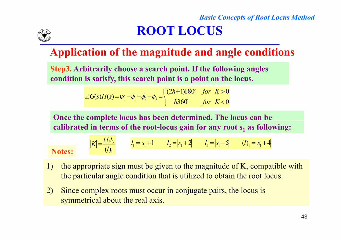
0180)12( Kforh
Step3. Arbitrarily choose a search point. If the following angles condition is satisfy, this search point is a point on the locus.
03600180)12(
)()( 3211 KforhKforh
sHsG
Once the complete locus has been determined. The locus can be pcalibrated in terms of the root-locus gain for any root s1 as following:
321
)(llllK 4)(521 11131211 slslslsl1)(l
1) the appropriate sign must be given to the magnitude of K, compatible with the particular angle condition that is utilized to obtain the root locus
Notes:
the particular angle condition that is utilized to obtain the root locus.
2) Since complex roots must occur in conjugate pairs, the locus is symmetrical about the real axis.
43
symmetrical about the real axis.
Basic Concepts of Root Locus Method
ROOT LOCUS
)4( K
Application of the magnitude and angle conditions
K=∞
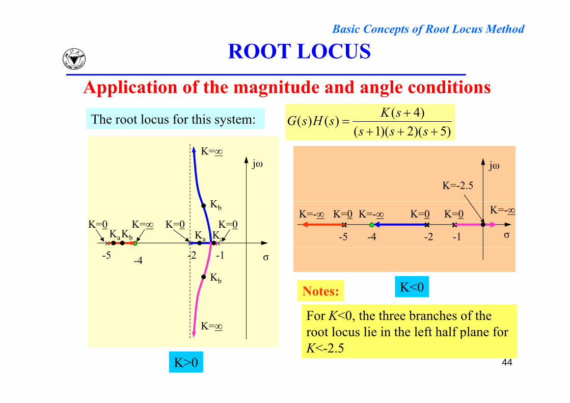
The root locus for this system:)5)(2)(1(
)4()()(
ssssKsHsG
jω
K
jω
K=-2.5
KaKb Ka Ka
Kb
K=0 K=0 K=0K=∞σ-1-2-4-5
K=0 K=-∞K=-∞ K=0 K=0K=-∞
σ-1-2-4-5
Kb K<0Notes:
K=∞For K<0, the three branches of the root locus lie in the left half plane for
Notes:
44K>0
pK<-2.5
Basic Concepts of Root Locus Method
ROOT LOCUS
)4( K
Application of the magnitude and angle conditions
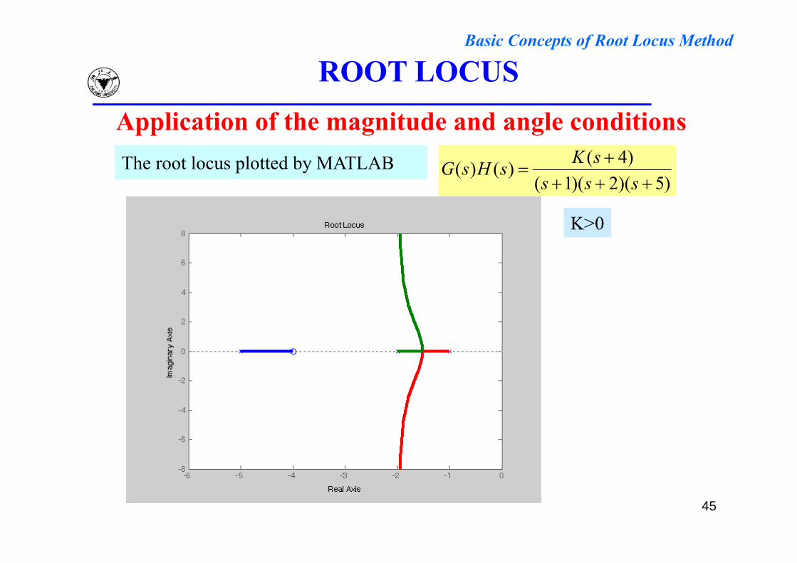
)5)(2)(1()4()()(
ssssKsHsGThe root locus plotted by MATLAB
K 0K>0
45

Basic Concepts of Root Locus Method
The End