CHAPTER 6 STORM SEWER HYDRAULICS - Nashville · Volume No. 2 Chapter 6 - 1 Metropolitan Nashville - Davidson County Stormwater Management Manual Volume 2 - Procedures May 2000 Chapter

Metropolitan Nashville - Davidson CountyStormwater Management ManualVolume 2 - Procedures

May 2000

CHAPTER 6STORM SEWER HYDRAULICS

Volume No. 2Chapter 6 - 1


May 2000

Chapter 6STORM SEWER HYDRAULICS

Synopsis

The general approach for storm sewer system design usually involves iterative sequences ofsystem layout, hydrologic and hydraulic calculations, and outfall design. Basic criteria andprocedures are presented for the design of storm sewer systems. Conditions requiring variancefrom these guidelines should be documented and approved by MWS.

6.1 Design Criteria

6.1.1 Return Periods

Closed conduits shall be designed for the total intercepted flow based on the design event (seeVolume 1, Section 6.3.1). In general, design event return periods are as follows:

Minor Facilities 10-yearMajor Facilities 100-year

Minor and major drainage facilities are defined in Volume 1.

6.1.2 Manning’s n Values

Values for Manning's roughness coefficient for concrete pipe, concrete box culvert, andcorrugated metal pipe (CMP) are given below:

Concrete pipes and box culverts n = 0.013(precast or cast-in-place)

CMP (non-spiral flow, annular n = 0.024corrugations)

CMP (full pipe spiral flow,helical corrugations)

Sizes 15-24" n = 0.017Sizes 30-54" n = 0.021Sizes 60-96"+ n = 0.024



May 2000

Additional details for selecting roughness coefficients for CMP can be obtained from FHWA-TS-80-216 (USDOT, FHWA, 1980).

Full pipe spiral flow occurs only for circular pipes longer than 20 diameters and free of sedimentbuildup when lining is not used. If the conditions for development of full pipe spiral flow arequestionable, the conservative use of the n value for non-spiral flow is more desirable.Conditions where full spiral flow may be appropriate are down drains, detention outlet pipes, andfree outlet or gravity storm sewer systems with a design velocity above 4 feet per second.

6.1.3 Slopes and Hydraulic Gradient

The standard recommended maximum and minimum slopes for storm sewers should conform tothe following criteria:

1. The maximum hydraulic gradient should not produce a velocity that exceeds 20 feet persecond.

2. The minimum desirable physical slope should be that which will produce a velocity of2.5 feet per second when the storm sewer is flowing full.

Systems should generally be designed for non-pressure conditions. When hydraulic calculationsdo not consider minor energy losses such as expansion, contraction, bend, junction, and manholelosses (see Section 6.4.2), the elevation of the hydraulic gradient for design flood conditionsshould be at least 1.0 foot below ground elevation. As a general rule, minor losses should beconsidered when the velocity exceeds 6 feet per second (lower if flooding could causecritical problems). If all minor energy losses are accounted for, it is usually acceptable for thehydraulic gradient to reach the gutter elevation. The maximum hydraulic gradient allowed is 5feet above the crown of the conduit (see Volume 1, Section 6.3.2).

6.1.4 Pipe Size and Length

A minimum pipe size of 15 inches is required when access spacing is 50 feet or less. Whenaccess spacing exceeds 50 feet, a minimum size of 18 inches is required. Designs should usestandard pipe size increments of 6 inches for pipes larger than 18 inches.

A minimum box culvert size of 3 by 3 feet for precast units and 4 by 4 feet for cast-in-place unitsis recommended. Increments of 1 foot in the height or width should be used above thisminimum. The span by height format is used for reporting box culvert dimensions, e.g., in thedimension 10 by 7, the span is 10 feet and the height is 7 feet.

Access spacing shall not exceed 400 feet for conduits less than 54 inches in diameter and shallnot exceed 800 feet without approval from MWS. The two materials for pipes allowed withinRight of Ways (or pipes that carry public water) are concrete and corrugated metal.



May 2000

6.1.5 Minimum Clearances

Minimum clearances for storm sewer pipe shall comply with the following criteria:

1. A minimum of 1 foot is required between the bottom of the road base material and theoutside crown of the storm sewer.

2. For utility conflicts that involve crossing a storm sewer alignment, the recommendedminimum design clearance between the outside of the pipe and the outside of anyconflicting utility should be 0.5 foot if the utility has been accurately located at the pointof conflict. If the utility has been approximately located, the minimum design clearanceshould be 1 foot. Electrical transmission lines or gas mains should never come into directcontact with the storm sewer.

3. Storm sewer systems should not be placed parallel to or below existing utilities in amanner that could cause utility support problems. The recommended clearance is 2 feetextending from each side of the storm sewer and 1:1 side slopes from the trench bottom.

4. When a sanitary line or other utility must pass through a manhole, a minimum 1-footclearance should be maintained between the bottom of the utility and the flow line of thestorm main, and greater clearance is recommended. Flow will be less obstructed whenthe utility is placed above or as close as possible to the crown of the pipe. The head losscaused by an obstruction should be accounted for. (Note: Gas mains shall not passthrough inlet and manhole structures.)

6.1.6 Inlet Location and Spacing

The location and spacing of inlets should be based on inlet capacity and width of spreadcalculations consistent with procedures and criteria presented in Chapter 4.

6.1.7 Easements

Easement requirements are given in Volume 1, Section 6.3.3.

6.2 General Approach

The design of storm sewer systems is usually an iterative process involving the following foursteps:

1. System Layout: Selection of inlet locations and development of a preliminary plan andprofile configurations consistent with design criteria in Section 6.1.



May 2000

2. Hydrologic Calculations: Determination of design flow rates and volumes (see Section6.3).

3. Hydraulic Calculations: Determination of pipe sizes required to carry design flow ratesand volumes, as discussed in Section 6.4.

4. Outfall Design: Outlet protection or detention/retention may be required because ofdownstream constraints; see Chapter 8 for detention/retention , Chapter 10 and Volume 4TCP-25 or PESC-07 for outlet protection.

6.3 Hydrologic Calculations

The two peak flow methods generally appropriate for hydrologic calculations for storm sewersystems are the Rational Method and the inlet hydrograph method. In general, as the time ofconcentration, drainage area, and variability in land use increase, more complex proceduresare warranted. A rule-of -thumb is that flood hydrograph procedures should be considered whenthe time of concentration goes beyond the range of 30 to 45 minutes. In addition, the size andcomplexity of the storm sewer system should be considered. (See Chapter 2 for additionalguidance on selecting hydrologic methods.)

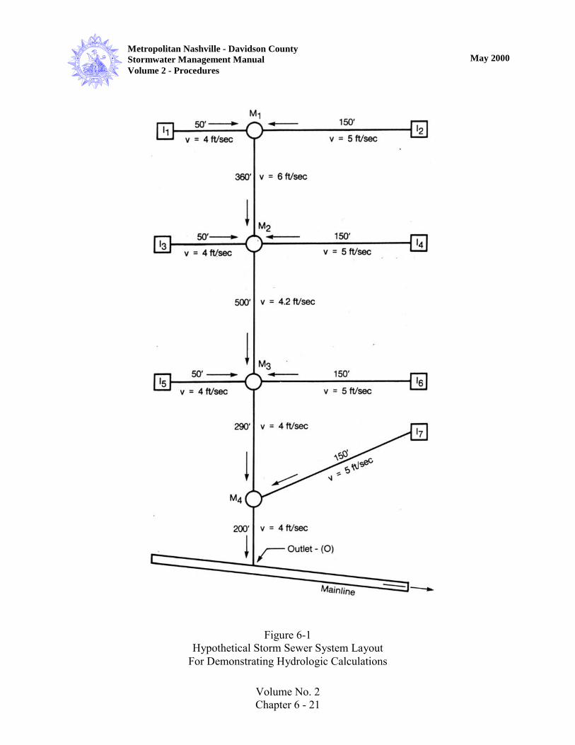
To demonstrate the application of the peak flow methods identified above and to provide a pointof comparison, the example storm sewer system layout shown in Figure 6-1 is evaluated below.Common data for calculating inlet flow rates are presented in Table 6-1.

6.3.1 Rational Method

The Rational Method, expressed in Chapter 2 as Equation 2-11, implicitly assumes that all runofffrom the tributary area is intercepted by the storm sewer system. Bypass must be accounted forby adjusting the tributary drainage area. The method requires a determination of the tributaryarea, time of concentration, rainfall intensity, and runoff coefficient at each design point.

The time of concentration is the sum of the inlet travel time and the storm sewer travel time andmust be calculated for each design point considered. Rainfall intensity is obtained from an IDFcurve (see Figure 2-1), based on the time of concentration and design frequency. The runoffcoefficient should be the composite factor based on tributary land use and soil conditions. Table2-3 (see Section 2.3.1) can provide a good starting point for selecting the runoff coefficient for a10-year return period, but other considerations should include examination of existing facilitiesand a comparison of historical performance with the results of design calculations, if possible.

Results of Rational Method calculations for the example storm sewer data presented in Figure 6-1 and Table 6-1 are shown in Table 6-2.



May 2000

6.3.2 Inlet Hydrograph Method

The inlet hydrograph method is a simplified approach that accounts for channel storage andappears to provide better estimates of observed peak runoff rates than the Rational Method (Jensand McPherson, 1964). The following equation is used to route intercepted flow for eachupstream inlet to the design point:

where:

Qo = Outflow peak runoff rate at the design point, in cfs

Qi = Intercepted flow peak runoff rate, in cfs

T = inlet travel time, in minutes

L = Length of storm sewer, in feet

v = Average velocity for storm sewer flow, in feet/minute

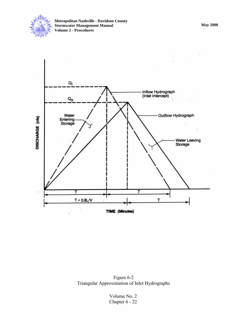
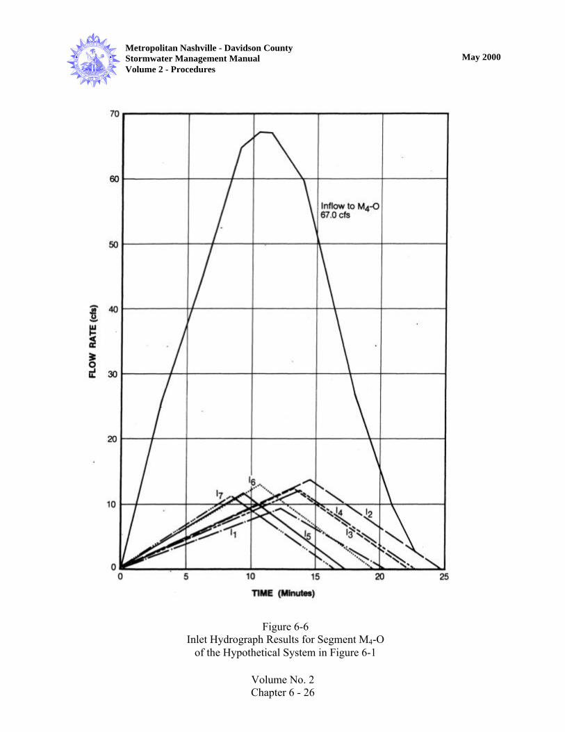
Having calculated the peak outflow, Qo, for intercepted flow from each inlet, Qi, the compositepeak flow at the design point is obtained by summing the ordinates of triangular hydrographs foreach inlet. This summation is accomplished graphically by drawing triangular hydrographs forthe outflow from each inlet with a peak of Qo, a rising limb time of T +0.8 (L/v), and a recessiontime of T. This procedure is illustrated in Figure 6-2, which also illustrates the inflowhydrograph with a peak flow rate equal to the inlet intercept and a time base of 2T. By plottingtriangular outflow hydrographs for each inlet tributary to the design point on the same scale, thecomposite hydrograph can be developed by summing hydrograph ordinates. Dividers arehelpful for accomplishing this summation.

Additional information on the use of the inlet hydrograph method can be found in publicationsby Jens and McPherson (1964) and Kaltenbach (1963).

Results of inlet hydrograph calculations for the example storm sewer data presented in Figure 6-1 and Table 6-1 are shown in Table 6-3. Graphical development of peak flows for each stormsewer segment is shown in Figures 6-3 through 6-6.

+=

vL

T

TQQ io

8.02

2(6-1)



May 2000

6.3.3 Example Comparison

Peak flow calculations from the two methods for the example storm sewer system in Figure 6-1are compared in Table 6-4. The inlet hydrograph method consistently gave the lowest peak flowresults, with the results obtained by the Rational Method corresponding closely. Pipe segmentsbetween inlets and manholes are not compared in Table 6-4 because each method produced thesame results (because 100 percent intercept was assumed).

The design flow for the pipe between the first two manholes, M1-M2, did not vary a great dealbetween methods. Beginning with pipe segment M2–M3, the inlet hydrograph method has lowerresults. The final pipe segment, M4-0, had a 13 percent reduction in peak flow rate for the inlethydrograph method, as compared to the Rational Method.

6.4 Hydraulic Calculations

Hydraulic calculations are used to size conduits to handle the design flows determined fromhydrologic calculations (see Section 6.3). The hydraulic capacity of a storm sewer conduit canbe calculated for the two types of conditions typically referred to as gravity and pressure flow.Hydraulic procedures provided in this section represent a summary of information frompublications by Brater and King (1976), Chow (1959), the American Society of Civil Engineers(1969), the University of Missouri (1958), and the American Iron and Steel Institute (1980).These publications should be consulted if additional details are required.

6.4.1 Pressure Versus Gravity Flow

Guidance is presented in Figure 6-7 for determining whether pressure or gravity flow conditionsoccur in a storm sewer system. In general, if the hydraulic grade line is above the crown of thepipe, pressure flow hydraulic calculations are appropriate. Conversely, if the hydraulic gradeline is below the crown of the pipe, gravity flow calculations are appropriate. Storm sewersystems should generally be designed as gravity systems (see Volume 1, Section 6.3.2).

For storm sewers designed to operate under pressure flow conditions, inlet surcharging andpossible manhole lid displacement can occur if the hydraulic grade line rises above the groundsurface. A design based on gravity conditions must be carefully planned as well, includingevaluation of the potential for excessive and inadvertent flooding created when a storm eventlarger than the design storm pressurizes the system.

Existence of the desired flow condition should be verified for design conditions. Storm sewersystems can alternate between pressure and gravity flow conditions from one section to another.



May 2000

The discharge point of the storm sewer system usually establishes a starting point for evaluatingthe condition of flow. If the discharge is submerged, as when the water level of the receivingwaters are above the crown of the storm sewer, the exit loss should be added to the waterlevel and calculations for head loss in the storm sewer system started from this point, asillustrated in Figure 6-7. If the hydraulic grade line is above the pipe crown at the next upstreammanhole, pressure flow calculations are indicated; if it is below the pipe crown, then gravity flowcalculations should be used at the upstream manhole.

When the discharge point is not submerged, a flow depth should be determined at a knowncontrol section to establish a starting elevation. As illustrated in Figure 6-7, the hydraulic gradeline is then projected from the starting elevation to the upstream manhole. Pressure flowcalculations may be used at the manhole if the hydraulic grade is above the pipe crown.

The assumption of straight hydraulic grade lines, as shown in Figure 6-7, is not entirely correct,since backwater and drawdown conditions can exist, but is generally reasonable. It is alsousually appropriate to assume the hydraulic grade calculations begin at the crown of the outletpipe for simple non-submerged systems. If additional accuracy is needed, as with very largeconduits or where the result can have a significant effect on design, backwater and drawdowncurves should be developed.

6.4.2 Energy Losses

The following energy losses should be considered for storm sewer systems:

1. Friction2. Entrance3. Exit

Additional energy loss parameters should be evaluated for complex or critical systems. Thefollowing losses are especially important when failure to handle the design flood has thepotential to flood offsite areas:

1. Expansion2. Contraction3. Bend4. Junction and manhole

Friction Loss

The energy loss required to overcome friction caused by conduit roughness is generallycalculated as:

gv

R

LnH

229 2

33.1

2

f

= (6-2)



May 2000

where:

Hf = Energy loss due to friction, in feet

n = Manning's roughness coefficient

L = Conduit length, in feet

R = Hydraulic radius of conduit, in feet

v = Average velocity, in feet/second

g = Acceleration due to gravity, 32.2 feet/second2

Entrance, Exit, Expansion, Contraction, and Bend Losses

These head losses due to pipe form conditions are generally calculated as:

where:

HL = Head loss due to pipe form conditions, in feet

K = Loss coefficient for pipe form conditions



The loss coefficient, K, is different for each category of pipe form loss and should be based onoperating characteristics of the specific system. Values for the entrance loss coefficient are thesame as those developed for culverts (see Chapter 5). Expansion and contraction losscoefficients for circular pipes can be selected based on data from Brater and King (1976)presented in Tables 6-5 and 6-6.

The bend loss coefficient for storm sewer systems can be evaluated using Figure 6-8, whichprovides various relationships between the angle of a bend and the loss coefficient.Relationships are presented for bends at manholes with and without deflectors, and for curveddrain alignments with r/D values equal to 2 and greater than or equal to 6.

gv

KH L 2

2

= (6-3)



May 2000

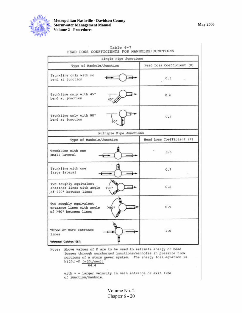
Junction and Manhole Losses

Losses associated with junctions and manholes should be evaluated with the procedures reportedby the University of Missouri (1958). Although details of the procedures are not given in thismanual, the application of important results is discussed below and head loss coefficients fortypical manholes and junctions are presented in Table 6-7.

For straight flow-through conditions, the University of Missouri (1958) indicates that pipesshould be positioned vertically between the limits of inverts aligned or crowns aligned. Anoffset in the plan is allowable, provided that the projected area of the smaller pipe falls withinthat of the larger. It is probably most effective to align the pipe inverts, as the manhole bottomwill then support the bottom of the jet issuing from the upstream pipe.

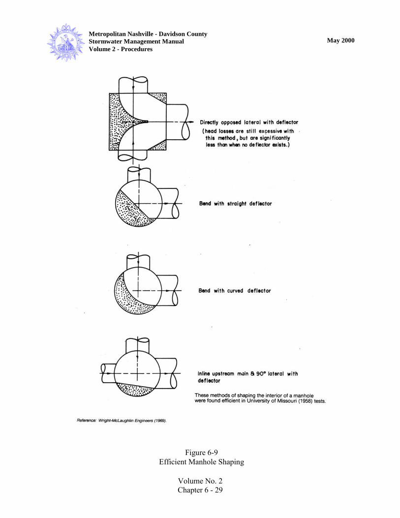
When two laterals intersect at a manhole, pipes should not be oppositely aligned, since the jetscould impinge upon each other. If directly opposing laterals are necessary, the installation of adeflector (as shown in Figure 6-9) will significantly reduce losses. The research conducted onthis type of deflector is limited to the ratios of outlet pipe to lateral pipe diameters equal to 1.25.In addition, lateral pipes should be located such that their centerlines are separated laterally by atleast the sum of the two lateral pipe diameters.

Jets from upstream and lateral pipes must be considered when attempting to shape the inside ofmanholes. Results reported by the University of Missouri (1958) for pressurized pipe flowconditions indicate that very little, if anything, is gained by shaping the bottom of a manhole toconform to the pipe invert. Shaping the manhole bottom to match the pipe invert may even bedetrimental when pressurized laterals flowing full are involved, as the shaping tends todeflect the jet upwards, causing unnecessary head loss. Limited shaping of the manhole bottomfor open channel flow conditions is required.

Figure 6-9 depicts several types of deflectors that can be efficient in reducing losses at junctionsand bends for full flow conditions. In all cases, the bottoms are flat or only slightly rounded (tohandle low flows). As a contrast, several inefficient manhole shapes are shown in Figure 6-10.Several of these inefficient devices would appear to be improvements, indicating that specialshapings deviating from those in Figure 6-9 should be used with caution.

6.4.3 Gravity Flow

The capacity of storm sewers designed to operate under gravity flow conditions should be sizedusing the following form of Manning's Equation:

2/13/2592.0SD

nv = (6-4)



May 2000

Q = vA (6-5)

where:

Q = Design flow rate, in cfs

v = Average velocity of flow, in feet/second


D = Pipe diameter, in feet

A = Cross-sectional area, in square feet

S= Slope of the energy gradient, in feet/foot

Storm sewer capacity calculations based on Manning's Equation can be accomplished usingFigures 6-11, 6-12, and 6-13 as discussed below or procedures published by Brater and King(1976), the American Concrete Pipe Association (1978 and 1980), Chow (1959), and theAmerican Iron and Steel Institute (1980).

Nomograph

The following steps are used for solving Manning's Equation using the circular pipe nomographin Figure 6-11:

1. Determine input data, including slope in feet/foot, Manning's n value, and pipe diameterin inches or feet.

2. Connect a line from the slope scale, Point 1, to the Manning's n scale, Point 2, and notethe point of intersection on the turning line, Point 3.

3. Connect a line from the pipe diameter, Point 5, to the point of intersection obtained inStep 2, Point 3.

4. Extend the line from Step 3 to the discharge and velocity scales to read the discharge atPoint 4 and the velocity at Point 6.

2/13/8465.0SD

nQ = (6-6)



May 2000

Partial Flow Charts

For partial flow in a circular pipe. Figures 6-12 and 6-13 can be used for capacity and velocitycalculations as follows:

1. Determine input data including design discharge, Q, Manning's n value, pipe diameter, D,and channel slope, S.

2. Calculate the circular pipe conveyance factor using the equation:

where:

Kp = Circular pipe open channel conveyance factor

Q = Discharge rate for design conditions, in cfs

n = Manning's roughness coefficient (see Section 6.1.2)

D = Pipe diameter, in ft

S = Slope of the energy grade line, in feet/foot

3. Enter the x-axis of Figure 6-12 with the value of Kp calculated in Step 2 and run a linevertically to the curve.

4. From the point of intersection obtained in Step 3, run a horizontal line to the y-axis andread a value of the normal depth of flow over the pipe diameter, d/D.

5. Multiply the d/D value from Step 4 by the pipe diameter, D, to obtain the normal depth offlow.

6. Enter the y-axis of Figure 6-13 with the d/D value from Step 4 and run a line horizontallyto the curve.

7. From the point of intersection obtained in Step 6, run a line vertically downward and reada value of kv, which equals vn/D2/3 S1/2, from the x-axis.

2/13/8 SD

QnK p = (6-7)



May 2000

8. Calculate the average velocity by the equation:

where:


kv = Pipe velocity factor from Figure 6-13 (Step 7)

D = Pipe diameter, in feet

S = Slope of the energy grade line, in feet/foot

n = Manning's roughness coefficient (see Section 6.1.2)

6.4.4 Pressure Flow

The capacity of storm sewers designed to operate under pressure flow conditions can be sizedusing inlet and outlet control nomographs developed for the evaluation of culverts (see Chapter5). A more general procedure involves the application of the Energy Equation, which can bedeveloped to consider unsteady flow conditions.The capacity of storm sewers flowing full can be evaluated by considering velocity head, pipeform, and friction losses, expressed as:

H = Hv + HL + Hf (6-9)

or

where:

H = Head, determined as the difference between the hydraulic grade line at thedownstream pipe and the energy grade line at the upstream pipe, in feet

Hv = Velocity head, in feet

HL = Head loss due to pipe form conditions, in feet

gv

R

LnKH L 2

2912

33.1

2

++= (6-10)

n

SDKv v

2/13/2

= (6-8)



May 2000

Hf = Head loss due to friction, in feet

KL = Loss coefficient for pipe form losses

n = Manning’s roughness coefficient

L = Length of storm sewer segment, in feet

R = Hydraulic radius, in feet



If H can be determined, the storm sewer capacity is calculated by rearranging Equation 6-8 asfollows:

or

where:


Q = Storm sewer capacity, in cfs


H = Head, determined as the difference between the hydraulic grade line at thedownstream pipe and the energy grade line at the upstream pipe, in feet

KL = Loss coefficient for pipe form losses


L = Length of storm sewer segment, in feet

2/1

33.1

22912

++÷=

R

LnKgHv L

(6-11)

2/1

33.1

22912

++÷=

R

LnKgHAQ L

(6-12)



May 2000

R = Hydraulic radius, in feet

The determination of H will generally involve an evaluation of energy losses to establish thehydraulic and energy gradients. Since the velocity is a required input to energy loss calculations,an iterative trial and error procedure is generally required.

6.5 Construction and Maintenance Considerations

An important step in the design process involves identifying whether special provisions arewarranted to properly construct or maintain proposed facilities. Maintenance concerns of stormsewer system design focus on adequate physical access for cleaning and repair. Volume 4 CP-18and 20 should be considered as a part of the design process.



May 2000

Table 6-1DATA FOR DEMONSTRATING THE APPLICATION OF STORM SEWER HYDROLOGIC METHODS

Inlet aDrainage Area

(acres)

Time ofConcentration

(minutes)

Rainfall bIntensity

(inches/hr)Runoff

CoefficientInlet Flow Rate c

(cfs)1 2.0 8.0 6.4 .9 11.52 3.0 10.0 6.1 .9 16.53 2.5 9.0 6.2 .9 14.04 2.5 9.0 6.2 .9 14.05 2.0 8.0 6.4 .9 11.56 2.5 9.0 6.2 .9 14.07 2.0 8.0 6.4 .9 11.5

a Inlet and storm sewer system configuration are shown in Figure 6-1.

b Data for example calculations only. See Chapter 2 for Nashville IDF data.

c Calculated using the Rational Equation (see Chapter 2).

Table 6-2RESULTS OF RATIONAL METHOD CALCULATIONS FOR THE

HYPOTHETICAL STORM SEWER SYSTEM IN FIGURE 6-1

Storm SewerSegment

Tributary Area a

(acres)

Time ofConcentration b

(minutes)

RainfallIntensity c(inches/hr)

RunoffCoefficient

DesignFlow Rate (cfs)

I1 – M1 2.0 8.0 6.4 .9 11.5I2 – M1 3.0 10.0 6.1 .9 16.5

M1 – M2 5.0 10.5 6.0 .9 27.0I3 – M2 2.5 9.0 6.2 .9 14.0I4 – M2 2.5 9.0 6.1 .9 13.7

M2 – M3 10.0 11.5 5.7 .9 51.3I5 – M3 2.0 8.0 6.4 .9 11.5I6 – M3 2.5 9.0 6.2 .9 14.0

M3 – M4 14.5 13.5 5.4 .9 70.5I7 – M4 2.0 8.0 6.4 .9 11.5M4 – O 16.5 14.7 5.2 .9 77.2

a Tributary area data are presented in Table 6-1.b See Figure 6-1 for details.c Data for example calculations only. See Chapter 2 for Nashville IDF data.



May 2000

Table 6-3RESULTS OF INLET HYDROGRAPH CALCULATIONS FOR THE

HYPOTHETICAL STORM SEWER SYSTEM IN FIGURE 6-1

A. Segment M1 – M2

Inlet2T

(minutes)L/v

(minutes) vL

T

T

8.02

2

+ Qi(cfs)

Qo(cfs)

12

1620

0.20.5

0.990.98

11.516.5

11.416.2

Inflow to Segment M1 – M2 = 24.5 cfs (from Figure 6-3)

B. Segment M2 – M3

Inlet2T

(minutes)L/v

(minutes) vL

T

T

8.02

2

+ Qi(cfs)

Qo(cfs)

1234

16201818

1.21.50.20.5

0.940.940.990.98

11.516.514.014.0

10.815.513.913.7

Inflow to M2 – M3 = 50.0 cfs (from Figure 6-4)

C. Segment M3 – M4

Inlet2T

(minutes)L/v

(minutes) vL

T

T

8.02

2

+ Qi(cfs)

Qo(cfs)

123456

162018181618

3.23.52.22.50.20.5

0.860.880.910.900.990.98

11.516.514.014.011.514.0

9.914.512.712.611.413.7

Inflow to M3 – M4 = 65.5 cfs (from Figure 6-5)



May 2000

Table 6-3(Continued)

D. Segment M4 – O

Inlet2T

(minutes)L/v

(minutes)

vL

T

T

8.02

2

+ Qi(cfs)

Qo(cfs)

1234567

16201818161816

4.44.73.23.71.41.70.5

0.820.840.880.860.930.930.98

11.516.514.014.011.514.011.5

9.413.912.312.010.713.011.3

Inflow to M4 – 0 = 67.0 cfs (from Figure 6-6)

Note: Qi values are calculated in Table 6-1.

168.02

2−

+= Equation

vL

T

TQQ io



May 2000

Table 6-4COMPARISON OF HYDROLOGIC METHODS FOR THE HYPOTHETICAL

STORM SEWER SYSTEM IN FIGURE 6-1

Storm Sewer aSegment

Rational Method b(cfs)

Inlet Hydrograph c(cfs)

M1 – M2

M2 – M3

M3 – M4

M4 – O

27.051.370.577.2

24.550.065.567.0

a Storm sewer configuration is shown in Figure 6-1.

b Results obtained from Table 6-2.

c Results obtained from Table 6-3.

Table 6-5VALUES OF K2 FOR DETERMINING LOSS OF HEAD DUE TO

SUDDEN EXPANSION IN PIPES, FROM THE FORMULAH2 = K2 (V1 2/2g)

d2/d1 = Ratio of larger pipe to smaller pipe diameter

v1 = Velocity in smaller pipe

Velocity, v1 (feet/second)

1

2

d

d

2 3 4 5 6 7 8 10 12 15 20 30 40

1.21.41.61.82.0

.11

.26

.40

.51

.60

.10

.26

.39

.49

.58

.10

.25

.38

.48

.56

.10

.24

.37

.47

.55

.10

.24

.37

.47

.55

.10

.24

.36

.46

.54

.10

.24

.36

.46

.53

.09

.23

.35

.45

.52

.09

.23

.35

.44

.52

.09

.22

.34

.43

.51

.09

.22

.33

.42

.50

.09

.21

.32

.41

.48

.08

.20

.32

.40

.47

2.53.04.05.0

10.0∞

.74

.83

.92

.961.001.00

.72

.80

.89

.93

.991.00

.70

.78

.87

.91

.96

.98

.69

.77

.85

.89

.95

.96

.68

.76

.84

.88

.93

.95

.67

.75

.83

.87

.92

.94

.66

.74

.82

.86

.91

.93

.65

.73

.80

.84

.89

.91

.64

.72

.79

.83

.88

.90

.63

.70

.78

.82

.86

.88

.62

.69

.76

.80

.84

.86

.60

.67

.74

.77

.82

.83

.58

.65

.72

.75

.80

.81

Reference: Brater and King (1976).



May 2000

Table 6-6VALUES OF K3 FOR DETERMINING LOSS OF HEAD DUE TOSUDDEN CONTRACTION IN PIPES, FROM THE FORMULA

H3 = K3 (V2 2/2g)

d2/d1 = Ratio of larger pipe to smaller pipe diameter

v2 = Velocity in smaller pipe

Velocity, v2 (feet/second)

1

2

d

d

2 3 4 5 6 7 8 10 12 15 20 30 40

1.11.21.41.61.8

.03

.07

.17

.26

.34

.04

.07

.17

.26

.34

.04

.07

.17

.26

.34

.04

.07

.17

.26

.34

.04

.07

.17

.26

.34

.04

.07

.17

.26

.34

.04

.07

.17

.26

.33

.04

.08

.18

.26

.33

.04

.08

.18

.26

.32

.04

.08

.18

.25

.32

.05

.09

.18

.25

.31

.05

.10

.19

.25

.29

.06

.11

.20

.24

.27

2.02.22.53.0

.38

.40

.42

.44

.38

.40

.42

.44

.37

.40

.42

.44

.37

.39

.41

.43

.37

.39

.41

.43

.37

.39

.41

.43

.36

.39

.40

.42

.36

.38

.40

.42

.35

.37

.39

.41

.34

.37

.38

.40

.33

.35

.37

.39

.31

.33

.34

.36

.29

.30

.31

.33

4.05.0

10.0∞

.47

.48

.49

.49

.46

.48

.48

.49

.46

.47

.48

.48

.46

.47

.48

.48

.45

.47

.48

.48

.45

.46

.47

.47

.45

.46

.47

.47

.44

.45

.46

.47

.43

.45

.46

.46

.42

.44

.45

.45

.41

.42

.43

.44

.37

.38

.40

.41

.34

.35

.36

.38

Reference: Brater and King (1976).



May 2000



May 2000

Figure 6-1Hypothetical Storm Sewer System Layout

For Demonstrating Hydrologic Calculations



May 2000

Figure 6-2Triangular Approximation of Inlet Hydrographs



May 2000

Figure 6-3Inlet Hydrograph Results for Segment M1-M2

of the Hypothetical System in Figure 6-1



May 2000





May 2000





May 2000

Figure 6-6Inlet Hydrograph Results for Segment M4-O




May 2000

Figure 6-7Determination of Pressure vs. Open Channel Flow Conditions

in Storm Sewer Systems



May 2000

Figure 6-8Storm Sewer Bend Loss Coefficient



May 2000

Figure 6-9Efficient Manhole Shaping



May 2000

Figure 6-10Inefficient Manhole Shaping



May 2000

Figure 6-11Circular Pipe Nomograph for Solving Manning’s Equation



May 2000

Figu

re 6

-12

Circ

ular

Pip

e Pa

rtial

Flo

w C

apac

ity C

hart



May 2000

Figure 6-13Circular Pipe Partial Flow Velocity Chart

Documents

CHAPTER 6 STORM SEWER HYDRAULICS - Nashville · Volume No. 2 Chapter 6 - 1 Metropolitan Nashville - Davidson County Stormwater Management Manual Volume 2 - Procedures May 2000 Chapter