1

Chapter 6 Virtual Work Principles

Principle of virtual Displacement = stiffness method = Displacement method

Principle of virtual force = flexibility method = force method

The principle of virtual displacements finds its most powerful application in the development of approximate solutions.

Advantages:

Without the force-equilibrium, the governing equation ( )Ku P= can be obtained, assuming a displacement function.

Even a displacement function not satisfying the equilibrium can be used to obtain an approximate solution.

Principle of Virtual Displacement

int ( )virtual external work virtual internal work (virtual strain energy)

extW U or W WWU

δ δ δ δδδ

= =

==

2

W u Pδ δ= ⋅

= U Ud U

dδ δ ν δ δε σ

δε σ ν

= ∫ = ⋅

∫ ⋅

6.1 Principle of virtual Displacements – Rigid Bodies

0W Uδ δ= =

For a particle subjected to a system of force in equilibrium, the work due to a virtual displacement is zero.

1 2 and does not induce internal work because of the rigid body motion.v vδ δ

3

1 1 2 2 3 3

1 2

3 33 1 2

3 31 3 1 2 3 2

1 (satisfy the compatibility for rigid body)

1

1 0

y y y

y y y y

W F v F v P v

x xv v vL Lx xv v vL L

x xW F P v F P vL L

δ δ δ δ

δ δ δ

δ δ δ

δ δ δ

= + −

= − + = − +

= − − + − = // // 0 0

A particle is in equilibrium under the action of a system of forces if the virtual work is zero for every independent virtual displacement.

31 3

3 32

1y y

yy

xF PL

P xF

L

= −

=

4

Example 6.1

After releasing member force 3 6F − , lateral displacement 5uδ cause a rigid body motion which does not cause internal deformation and energy.

3 6

5 5 3 6 5

3 6

0 solve

1.52 ( ) ( ) ( ) 03.25

=2 3.25 P

W F

W P u P u F u

F

δ

δ δ δ δ

−

−

−

= ⇒

= + − =

5

6.2 Principle of virtual Displacements – Deformable bodies

Principle of virtual displacement for deformable bodies

W Uδ δ=

For a deformable structure in equilibrium under the action of a system of applied force, the external virtual work due to an admissible virtual displaced state is equal to the internal virtual work due to the same virtual displacements.

W U Ku Pδ δ= ⇒ =

General Mechanics Energy Principle

force – equilibrium principle of virtual displacement

Displacement – compatibility ⇒ Displacement - compatibility

force – Displ. Relationship force – Displ. Relationship

Since energy is expressed as displacement ｘ force, in order to satisfy

W Uδ δ= , at least internal force ≈ external force in average sense if the

6

displacement-compatibility is satisfied.

Internal force is defined as the function of the assumed displacement.

6.3 Virtual Displacement analysis procedure and Detailed Expressions

6.3.1 General procedure

The principle of virtual displacements finds its most powerful application in the development of approximate solutions.

Only displacement functions, which satisfy b/c, are required while force-equilibrium is assumed to be satisfied by using the condition of energy conservation.

6.3.2 Internal virtual work

1) Axial force member

( )virtual energy de

nsity= x x

Uδδε σ

Internal work is defined as the function of

displacement.

7

( ) =

=

= d

=

virtual ener

= ( ) ( )

gy

x x

L

x xo

L L

x xo o

U

UdV

dV

x

d u duEA dx EA dxdx dx

δ

δ

δε σ

δε σ

δδε ε

∫∫∫

∫ ∫

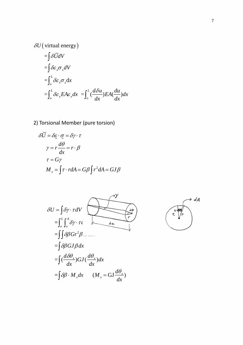
2) Torsional Member (pure torsion)

2

x

Udr rdx

G

M rdA G r dA GJ

δ δε σ δγ τθγ β

τ γ

τ β β

= ⋅ = ⋅

= = ⋅

=

= ⋅ = =∫ ∫

2

=

=

=

= ( ) ( )

= ( GJ )

L A

o o

x x

xx x

U dV

dAdx

Gr dAdx

GJ dx

d dGJ dxdx dx

dM dx Mdx

δ δγ τ

δγ τ

δβ β

δβ β

δθ θ

θδβ

= ⋅

⋅

⋅ =

∫∫ ∫∫ ∫∫

∫

∫

8

3) flexural member

2

2

x x

x

x x

U

d vy ydx

E Ey

δ δε σ δε σ

δδε δφ

σ ε φ

= ⋅ =

= − = −

= = −

2

2

2 2

2 2

=

=

= ( )

= EI

= ( )

x x

x xL A

A

z z

L

zo

L

z z zo

U dV

dA dx

Ey dA dx

EI dx y dA I

d v d v dxdx dx

M dx M EI

δ δε σ

δε σ

δφ φ

δφ φ

δ

δφ φ

=

=

=

∫∫ ∫∫ ∫∫ ∫

∫ ∫

∫

6.3.3 External virtual work

(or )

i iW u P u b dV

u b dx

δ δ δ

δ

= ∑ + ⋅

⋅

∫∫

Example 6.2

9

6.4 Construction of Analytical Solutions by the principle of virtual displacements

6.4.1 Exact solutions

2select u= x uL

which satisfy the B/C’s: 2

at 0 0at

x ux L u u= == =

2u= x uL

2x

du udx L

ε = =

2= xu uL

δ δ 21

x uL

δε δ=

0

2 20

2 2

=

( )

L

x x

L

U dV

EA dx

u uEA dxL L

EA u uL

δ δε σ

δε ε

δ

δ

⋅

=

=

=

∫∫

∫

10

2 2

2 2=

x

x

W u FEAU W F uL

LdEA

δ δ

δ δ

=

⇒ =

=

Why is 2= xu uL

exact displacement function?

The exact displacement function is the one that satisfies the force-equilibrium.

By equilibrium, 0xdF b dx+ =

xdFbdx

= −

When 0, 0xdFbdx

= =

( ) 0

duF A EA EAdx

d duEAdx dx

σ ε= ⋅ = =

⇒ =

11

When E and A are constant,

2

2

2

2 2

0 the condition for the exact displacement function

u= satisfies ( 0)

d udx

x d uuL dx

= ⇒

=

Virtual displacement with different B/C

displacement shape

yields the same equilibrium equation

U dVδ δεσ= ∫

For virtual displacement 1 2(1 )v

x xu u uL L

δ δ δ= − + Eq. 1

- Virtual displacement is applied to the equilibrium system and is not related to the actual displ. B/C. Thus vuδ in Eq. 1 is valid.

- 1 2 2 Reaction can be calculatedEAF F uL

= − = − ⇒

- 2vxu uL

δ δ= is a special case of Eq. 1

12

2

1 2

1 2 2 2

= ( )

=

v rr

r

d u du xU EA dx u udx dx L

u u duEA dxL L dxEA EAu u u uL L

δδ

δ δ

δ δ

= =

− +

− +

∫

∫

1 1 2 2

1 2

2 2

W u F u FEAU W F uL

EAF uL

δ δ δ

δ δ

= +

= ⇒ = −

=

If we use for both real displacement and virtual displacement,

1 2

1 2

1 2 1 2

(1 )

(1 )

= ( ) ( )

r

v

v r

x xu u uL L

x xu u uL L

d u duU EA dxdx dx

u u u uEA dxL L L L

δ δ

δδ

δ δ

= − +

= − +

=

− + − +

∫

∫

13

1 1 2 2

1 1 2

2 2 1

1 1

2 2

( )

( )

1 -1-1 1

W u F u FEAU W F u uL

EAF u uL

F uEAF uL

δ δ δ

δ δ

= +

= = −

= −

=

Different displacement shape for virtual displacement

22

2

( )

sin2

v

v

xu uL

xu uL

δ δ

πδ δ

= →

=

satisfy displacement boundary condition.

but not satisfy the force-equilibrium.

Real displacement 2rxu uL

=

v rd u duU EA dxdx dxδδ = ∫

Integration by part

2 2

2 20

0

' , ' = - '

= 0 0

=

v r

v r

Lr r r

v v

Lr

v

d u duU EA dxdx dx

d u dua b a b ab abdx dx

du d u d u dFEA u EA u dxdx dx dx dx

duEA udx

δδ

δ

δ δ

δ

=

= =

− = =

∫

∫ ∫

∫

14

This result indicates that Uδ is affected by the values at the starting and last points, regardless of the shape of the vu

Thus if virtual displacement vuδ satisfies the displacement B/C, any form of virtual displacement can be used.

(Here, 20 0 , v vx u x L u uδ δ δ= = = = )

However, the real displacement 2u ( )rx uL

= should satisfy

2

2 0 (when 0)rx

d u bdx

= = , which is the force-equilibrium condition.

2

2

2

2

v

r

xu uL

xu uL

δ δ =

=

2

2

sin( )2

sin( )2

v

r

xu uL

xu uL

πδ δ

π

= =

⇒ cannot get the exact solution, because 2

2 0rd udx

≠

If the chosen read displacements corresponds to stresses that satisfy identically the conditions of equilibrium, any form of admissible virtual displacement will suffice to produce the exact solution.

15

6.4.2 Approximate solutions and the significance of the chosen virtual displacements

Principle of virtual work is applicable to seeking approximate solutions for

Frame work Analysis: tapered section, nonlinearity, instability, dynamics

All finite element analysis

For example, tapered truss element.

Equilibrium condition

xdF bdx

= −

If 0xb = , 0dFdx

=

If 2xu uL

= is used,

2x

du uE E Edx L

σ ε= = =

16

But, 21 1(1 ) / = E (1 ) / 0

2 2x

xdF x u xd A dx d A dxdx L L L

σ = − − ≠

⇒ violate the force-equilibrium condition

Nevertheless, we can use the approximate displacement function

2xu uL

= which is exact only for prismatic elements.

2 21

12 2

2 2

12 2

21

2 2 2

2

= (1 )2

3 = 4

3 4

2for 3

L

o

L

o

x

x

x

d u duU EA dxdx dxu u xEA dxL L L

EAu uL

W u F

EAU W F uL

xu uL EAF u

Lxu uL

δδ

δ

δ

δ δ

δ δ

δ δ

=

−

= ⋅

= ⇒ =

= ⇒ = =

∫

∫

21

2 2

2

0.6817for sin

2

x

xu uL EAF u

x Lu uL

πδ δ

= ⇒ =

=

Exact solution = 120.721 EA u

L

17

Discussions

1) Although u is not exact displacement function,

W Uδ δ= (energy conservation) force to provide a basis for the calculation of the undetermined parameter 2u

2) Although the approximate real displacement cannot satisfy the equilibrium conditions at every locations, the enforcement of the condition W Uδ δ= results in average satisfaction of the equilibrium throughout the structure.

3) The standard procedure for choosing the form of virtual displacement is to adopt the same form as the real displacement for convenience and to make the stiffness matrix symmetric.

Requirement of displacement function (real displacement)

1) Displacement Boundary condition should be satisfied.

In case of 2-node truss element, there are two nodes. Thus, only two terms can be used when a polynomial equation is used.

For example 0 1u a a x= +

2 11 2 0 1 10, , , u ux u u x L u u a u a

L−

= = = = ⇒ = =

2) Rigid body motion (no strain) and constant strain should be described.

1 2

(nodal displacements) = ( , )u f

f u u=

18

0 1

0 1

(O.K)

= sin (Not OK)2

u a a x

u a a xLπ

= +

+

3) Force-equilibrium should be satisfied.

For axial force member

( )x xdF d dub EA bdx dx dx

= ⇒ =

1) is the essential condition to get at least an approximate solution

2) is the convergence condition to get a reasonably accurate solution by increasing the number of elements.

3) is the condition to obtain the exact solution.

Generally, virtual displacement function is the same as the real displacement Function.

⇒ symmetric matrix

Example 6.5

Rayleigh-Ritz method

1 2

1 2

2sin sin

, generalized displacements

solve approximate solution

x xa aL L

a a

W U

π πu

δ δ

= +

=

= ⇒

19

6.5 Principle of Virtual Force

Principle of Virtual Force

≡ flexibility method

≡ Force method

6.5.1 Equations of Equilibrium

The fundamental requirement on virtual force systems is that they meet the relevant conditions of equilibrium.

For axial force member,

/

x

x A

dF bdx

F Aσ

= −

=

For torsional member,

xx

dM mdx

= −

= xM rJ

τ

20

For flexural member,

2

2

0

0

y y y

yy

z z y

zy

zy

F dF b dxdF

bdx

M dM F dxdM Fdx

d M bdx

∑ = − + =

⇒ =

∑ = − ⋅ =

⇒ =

=

6.5.2 Characteristics of virtual force systems

External Equilibrium Equation. 0F∑ =

Internal Equilibrium Equation.

and =

xx

xx

y zy y

dF bdxdM mdx

dF dMb Fdx dx

= − = − =

21

Virtual complementary Strain energy

* *

1

U U dv

dv

E dv

δ δ

δσ ε

δσ σ−

=

= ⋅

=

∫∫∫

* *W Uδ δ= gives the conditions of compatibility.

The strains and displacements in a deformable system are compatible and consistent with the constraints if and only if the external complementary virtual work is equal to the internal complementary virtual work for every system of virtual force and stresses that satisfy the conditions of equilibrium.

Even if the real force state does not correspond to a deformational state that exactly satisfies compatibility, * *W Uδ δ= can be used to enforce an approximate satisfaction of the conditions of compatibility.

22

For axial force member,

* 1

1

( = )

1 d

x x

x x

U E dV

dVEA dxE

F FE E

F F xEA

δ δσ σ

δσ σ

δσ σ

δσ δσ

δ

−=

=

=

=

=

∫

∫

∫

∫

For torsional member

* 1

22

1

1

1 d

x

x x

x x

U E dV

M rdVG J

M r M dA dxGJ

M M xGJ

δ δσ σ

δτ τ τ

δ

δ

−=

= =

= ⋅

=

∫

∫

∫ ∫

∫

For flexural member

* 1

1

1

U E dV

MydVE I

M M dxEI

δ δσ σ

δσ σ σ

δ

−=

= = −

= ⋅

∫

∫

∫

23

6.5.4 Construction of Analytical Solutions by virtual force principle

Axial force member

*2

2 2

*2 2

* *2 2

xx x x

x x

x

x

FU F dx F FEALF F

EAW F u

LW U U FEA

δ δ

δ

δ δ

δ δ

= ⋅ =

=

= ⋅

= ⇒ =

∫

Flexural member

2

2

PM x

xM Pδ δ

=

= ⋅

*

2/2

0

3

2 4

48

MU M dxEI

xP P dxEI

P PEI

δ δ

δ

δ

=

= ⋅ ⋅

= ⋅

∫

∫

By using equilibrium equation with low orders, the solution can be found conveniently.

24

*

3* *

48

W P vPW U v

EI

δ δ

δ δ

= ⋅

= ⇒ =

If we set 1Pδ = ,

The principle of virtual force ≡ unit load method.

25

Discussion on virtual force system

* * * *U U U Uδ δ δ δ= = =① ② ③ ④

The force-equilibrium cause a relative displacement (deformation).

On the other hand, with different support conditions, the relative displacement could be the same when the force-equilibrium is the same.

26

Discussion on stiffness method vs flexibility method

For principle of virtual displacement

4

4

( 0)

W U

W dV

d vvEIv dxdx

δ δ

δ δεσ

δ

=

=

= =

∫

∫

v ⇒ 3rd order equation to satisfy the force-equilibrium

If the cross-section is variable along the length, v function becomes more complicated.

On the other hand, for principle of virtual force,

* *

*

W U

U dV

MM dVEI

δ δ

δ δσ ε

δ

=

= ⋅

=

∫

∫

M ⇒ 1st order equation for the determinate system.

As the element properties become more complicate, the flexibility method is easier in the derivation of the flexibility matrix and stiffness matrix.