Chapter 7: 2D and 3D Image Analysis by Gaussian–Hermite ...library.utia.cas.cz/separaty/2014/ZOI/flusser-0429813.pdf · 2D and 3D Image Analysis by Gaussian Hermite Moments 145

CHAPTER 7

2D and 3D Image Analysis by Gaussian�Hermite Moments

Bo Yang, Tomas Suk, Mo Dai and Jan Flusser

This chapter introduces 2D and 3D Gaussian�Hermite moments and rotation invari-ants constructed from them. Thanks to their numerical stability, Gaussian�Hermitemoments provide better reconstruction and recognition power than the geometric andmost of other orthogonal moments while keeping the simplicity of design of the invari-ants. This is illustrated by experiments on real 2D and 3D data.

7.1 Introduction

Although moments have been used in many image analysis tasks and areas, probablytheir most important and most frequent application is in object recognition. The key

Bo Yang, Tomas Suk, Jan FlusserInstitute of Information Theory and Automation of ASCR182 08 Prague 8, Czech Republice-mail: {yang, suk, �usser}@utia.cas.cz

Mo DaiENSEGID, Institut Polytechnique de Bordeaux 1Allee Daguin, 33607 Pessac Cedex, Francee-mail: [email protected]

Editor: G.A. Papakostas, Moments and Moment Invariants - Theory and Applications

DOI: 10.15579/gcsr.vol1.ch7, GCSR Vol. 1, c©Science Gate Publishing 2014143

144 B. Yang et al.

point is to �nd descriptors that can represent the object regardless of certain trans-formations and/or deformations. Moment invariants were proved to be very powerfultools for feature representation and it has been demonstrated many times that momentinvariants perform e�ectively in object recognition [7].

So far, various kinds of moment invariants to spatial transformations of the objecthave been proposed. Among all transformations that have been studied in this context,rotation plays a central role. Being a part of rigid-body transformation, object rotationis present almost in all applications, even if the imaging system is well set up and theexperiment has been prepared in a laboratory. On the other hand, rotation is not trivialto handle mathematically, unlike for instance translation and scaling. For these tworeasons, invariants to rotation have been in focus of researchers since the beginning.

The development of rotation invariants in 2D space has a long history. As earlyas in 1962, Hu �rst derived seven rotation invariants that formed an incomplete anddependent system [12]. After Hu, various approaches to the theoretical derivation ofmoment-based rotation invariants were published. Li employed Fourier-Mellin trans-formation to derive rotation invariants up to order nine [17]. Wong et al., on theother hand, derived the rotation invariants up to order �ve based on the theory ofalgebraic invariants [31]. Flusser o�ered the solution for complete and independentset constructed from complex moments [5]. Zernike moments were also consideredfor developing rotation invariants. Khotanzad and Hong pointed out that magnitudesof Zernike moments possess rotation invariance [16]. Wallin and Kubler formulatedan approach to derive a complete set of rotation invariants from Zernike moments[29]. Some other polynomial bases (Legendre, Krawtchouk, Gaussian�Hermite) wereemployed in a similar manner [10, 37, 36].

With the rapid progress of applied mathematics, computer science and sensor tech-nology, 3D imaging comes into engineering and practice. Undoubtedly, developingrotation invariants for 3D images has become a hot topic in the computer vision com-munity. However, 3D rotation is more di�cult to handle than its 2D counterpart,since it has three independent parameters. That is probably why only few papers on3D rotation moment invariants have appeared so far. The �rst attempts to derive3D rotation moment invariants are relatively old. Sadjadi and Hall explored ternaryquadratics extensively and derived three translation, rotation and scaling (TRS) mo-ment invariants. Their derivation was accomplished by using the invariant propertiesof the coe�cients in a ternary form [24]. Guo proved Sadjadi and Hall's results inthe di�erent way and he derived more invariants to translation and rotation in 3Dspace [9]. Cyganski and Orr applied tensor theory to derive 3D rotation invariants[2]. This method was also mentioned by [23], who used invariant image features torecognize planar objects. Xu and Li developed the invariants in both 2D and 3D spacebased on geometric primitives such as distance, area, and volume [32]. Galvez andCanton [8] and Canterakis [1] employed normalization approaches for constructing 3Dmoment invariants, which overcame the necessity of an explicit deriving the invariantsbut introduced potential numerical instability. Another method to derive 3D rota-tion invariants is based on complex moments [18, 6]. Several application papers werepublished, for example [19], where the authors used 3D TRS invariants for tests ofhandedness and sex from MRI snaps of brains as well as two other papers [14] and[28] discussing utilization of invariants in registration. Most recently, [26] proposed an

2D and 3D Image Analysis by Gaussian�Hermite Moments 145

automatic algorithm to generate 3D rotation invariants from geometric moments upto an arbitrary order.

Although moments are probably the most popular 3D shape descriptors, it shouldbe mentioned that they are not the only features providing rotation invariance. Forexample, Kakarala and Mao used the bispectrum, well-known from statistics for featurecomputation [13]. Kazhdan used an analogy of phase correlation based on sphericalharmonics for comparison of two objects [14]. In this particular case it was usedfor registration, but can be also utilized for recognition. In [15], the authors usedamplitude coe�cients as the features. Fehr used the power spectrum and bispectrumcomputed from a tensor function describing an object composed of patches [3]. In[4] the same author employed local binary patterns and in [25] he used local sphericalhistograms of oriented gradients.

There have been numerous discussions what kind of moments (i.e. what polyno-mial basis) provide the best performance. The criteria could be discrimination andreconstruction power, robustness to noise, computational e�ciency, and also suitabil-ity and accessibility for theoretical considerations. Traditional geometric and complexmoments are excellent for theoretical analysis but their numerical properties are notoptimal. On the other hand, the main advantage of orthogonal moments is their bet-ter numerical stability, limited range of values and existing recurrent relations for theircalculation. Note that there is no di�erence from theoretical point of view becauseany two polynomial bases of the same degree are equivalent. Hence, several authorshave tried to derive the 2D invariants from orthogonal moments. In 3D, however,the situation is more di�cult than in 2D, but one can still expect that 3D orthogonalmoments preserve their favorable numerical properties.

Both in 2D and 3D, there exist polynomials orthogonal inside a unit ball and othersthat are orthogonal on a unit cube. Seemingly, the polynomials de�ned on a unitball are more convenient for deriving rotation invariants because the ball is mappedonto itself and the polynomials are transformed relatively easily under rotation. Theinvariance is achieved by proper phase cancellation. The most popular basis of thiskind is the Zernike basis. However, real images coming from CT and MRI are de�nedon a cube and must be mapped into a unit ball before the moments are calculated.Such mapping requires resampling which always lead to a loss of precision.

Polynomial system orthogonal on a cube is (mostly but not necessarily) a productof three 1D polynomials. Since 1D orthogonal polynomials can be evaluated by e�-cient recurrent formulas, we can expect good numerical stability. On the other hand,derivation of invariants is in general very di�cult, because the basis polynomials aretransformed in a complicated way under rotation.

In this chapter we show that Gaussian�Hermite moments could be a good choice.Gaussian�Hermite basis is orthogonal on a cube which implies good numerical proper-ties. At the same time, Gaussian�Hermite polynomials are transformed under rotationin the same way as the monomials xpyq. Thanks to this, the respective rotationinvariants have the same forms as the rotation invariants from geometric moments.Under our knowledge, Gaussian�Hermite polynomials are the only ones showing thisproperty. This is an important conclusion valid in both 2D and 3D which allows usto reduce rotation invariant derivation from Gaussian�Hermite moments to that fromgeometric moments, which is much easier to accomplish but we still bene�t from the

146 B. Yang et al.

numerical stability of Gaussian�Hermite moments.The chapter is organized as follows. First we introduce Gaussian�Hermite polynomi-

als and moments. Then we formulate the central Theorem on the form of Gaussian�Hermite rotation invariants in 2D and 3D. Finally, we demonstrate the invarianceproperty and the discrimination power on simulated as well as real 2D and 3D data.

7.2 Gaussian�Hermite Moments

Before we discuss Gaussian�Hermite moments, it is necessary to introduce Hermitepolynomials �rstly. Hermite polynomials are orthogonal polynomials de�ned on theinterval (−∞,∞)

Hp(x) = (−1)p exp (x2)dp

dxpexp (−x2). (7.1)

It can be e�ciently computed by the following 3-term recurrence relation

Hp+1(x) = 2xHp(x)− 2pHp−1(x) for p ≥ 1, (7.2)

with the initial conditions H0(x) = 1 and H1(x) = 2x. Hermite polynomials areorthogonal when weighted by a Gaussian function

ˆ ∞−∞

Hp(x)Hq(x) exp (−x2)dx = 2pp!√πδpq, (7.3)

where δpq is the Kronecker delta. The basis functions we use for the de�nition ofGaussian�Hermite moments are normalized versions of Hermite polynomials. Hermitepolynomials are scaled and modulated by a Gaussian

Hp(x;σ) =1√

2pp!√πσ

Hp

(xσ

)exp

(− x2

2σ2

). (7.4)

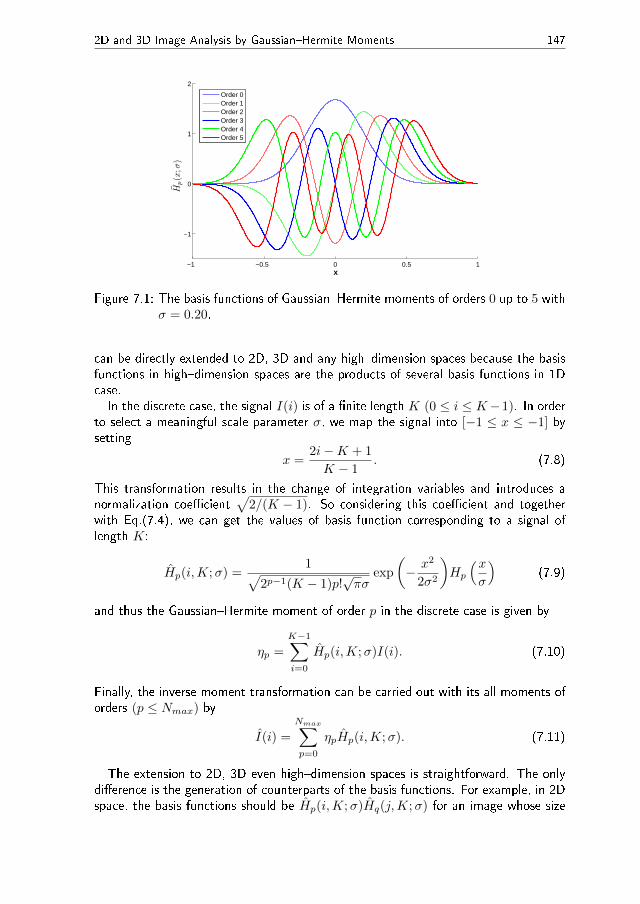
The scaling parameter σ is common to both factors. Figure 7.1 shows the basisfunctions of orders 0 up to order 5. Obviously, Eq.(7.4) is not only orthogonal butalso orthonormal, which means that

ˆ ∞−∞

Hp(x;σ)Hq(x;σ)dx = δpq. (7.5)

Given any image function f(x, y) its Gaussian�Hermite moments are therefore de�nedas

ηpq =

ˆ ∞−∞

ˆ ∞−∞

Hp(x;σ)Hq(y;σ)f(x, y)dxdy. (7.6)

For a 3D image f(x, y, z), its Gaussian�Hermite moments are computed directly by

ηpqr =

ˆ ∞−∞

ˆ ∞−∞

ˆ ∞−∞

Hp(x;σ)Hq(y;σ)Hr(z;σ)f(x, y, z)dxdydz. (7.7)

Discrete implementation of Gaussian�Hermite moments is mainly focused on thediscretization of the basis functions. Here we only discuss the 1D case. The results


−1 −0.5 0 0.5 1

−1

0

1

2

x

Hp(x;σ

)

Order 0Order 1Order 2Order 3Order 4Order 5

Figure 7.1: The basis functions of Gaussian�Hermite moments of orders 0 up to 5 withσ = 0.20.

can be directly extended to 2D, 3D and any high�dimension spaces because the basisfunctions in high�dimension spaces are the products of several basis functions in 1Dcase.In the discrete case, the signal I(i) is of a �nite length K (0 ≤ i ≤ K−1). In order

to select a meaningful scale parameter σ, we map the signal into [−1 ≤ x ≤ −1] bysetting

x =2i−K + 1

K − 1. (7.8)

This transformation results in the change of integration variables and introduces anormalization coe�cient

√2/(K − 1). So considering this coe�cient and together

with Eq.(7.4), we can get the values of basis function corresponding to a signal oflength K:

Hp(i,K;σ) =1√

2p−1(K − 1)p!√πσ

exp

(− x2

2σ2

)Hp

(xσ

)(7.9)

and thus the Gaussian�Hermite moment of order p in the discrete case is given by

ηp =

K−1∑

i=0

Hp(i,K;σ)I(i). (7.10)

Finally, the inverse moment transformation can be carried out with its all moments oforders (p ≤ Nmax) by

I(i) =

Nmax∑

p=0

ηpHp(i,K;σ). (7.11)

The extension to 2D, 3D even high�dimension spaces is straightforward. The onlydi�erence is the generation of counterparts of the basis functions. For example, in 2Dspace, the basis functions should be Hp(i,K;σ)Hq(j,K;σ) for an image whose size

148 B. Yang et al.

is K ×K pixels. In 3D space, they should be Hp(i,K;σ)Hq(j,K;σ)Hr(k,K;σ) foran image in a K ×K ×K voxels cube.

7.3 Rotation Invariants of Gaussian�Hermite

Moments

Gaussian�Hermite polynomials belong to the family of functions orthogonal on a squarein 2D and on a cube in 3D. Generally, it is di�cult to derive rotation invariants fromsuch moments because they transform themselves under rotation in a complicatedmanner. That is why most authors, when dealing with orthogonal moments, havepreferred polynomial systems orthogonal on a unit disc, such as Zernike and Pseudo-Zernike polynomials, where the invariance can be easily achieved by a proper phasecancellation. However, working with these polynomials requires image mapping intothe unit disc, which introduces resampling errors.In case of traditional geometric and complex moments, the rotation invariants are

known and comprehensively studied [7]. In this section we derive rotation invariantsfrom Gaussian�Hermite moments. We accomplish this using an interesting propertyof Hermite polynomials. We show that Gaussian�Hermite moments are transformedunder rotation in exactly the same way as geometric moments. This property enablesus to construct rotation invariants from Gaussian�Hermite moments in both 2D and3D cases indirectly and very easily.

7.3.1 Rotation Invariants in 2D Case

7.3.1.1 Mathematical Preliminaries

We de�ne non�coe�cient Gaussian�Hermite moments as

ηpq =

ˆ ∞−∞

ˆ ∞−∞

Hp(x;σ)Hq(y;σ)f(x, y)dxdy, (7.12)

with

Hp(x;σ) =

√2pp!√πσHp(x;σ). (7.13)

In order to achieve translation invariance, we use central moments

ηpq =

ˆ ∞−∞

ˆ ∞−∞

Hp(x− x0;σ)Hq(y − y0;σ)f(x, y)dxdy, (7.14)

where x0 = m10/m00 and y0 = m01/m00 are computed by the geometric moments

mpq =

ˆ ∞−∞

ˆ ∞−∞

xpyqf(x, y)dxdy, (7.15)

In 2D space, there is only one parameter θ determining the rotation. Yang et al.discovered an important rotation property of Hermite polynomials [36].


Theorem 1. Let p, q be two non�negative integers. Let the coordinates be rotatedas (

xy

)=

(cos θ − sin θsin θ cos θ

)(xy

)(7.16)

Then the following equation holds

xpyq =

p+q∑

r=0

k(r, p, q, θ)xp+q−ryr, (7.17)

where k(r, p, q, θ) is a coe�cient which is determined by p, q, and θ. Moreover theproduct of Hermite polynomials can also be expressed as:

Hp(x)Hq(y) =

p+q∑

r=1

k(r, p, q, θ)Hp+q−r(x)Hr(y). (7.18)

The proof of Theorem 1 can be found in Appendix of [36].Assume an original image f(x, y) is rotated by angle θ. Here, we use fθ to denote

the rotated image. After rotation the original coordinates (x, y) are changed to (x, y).According to Eq.(7.12), non�coe�cient Gaussian�Hermite moments of fθ are thereforecomputed by

ηθpq =

ˆ ∞−∞

ˆ ∞−∞

Hp(x;σ)Hq(y;σ)fθ(x, y)dxdy. (7.19)

Rotation does not change image intensity function and the scaling of image, whichmeans {

fθ(x, y) = f(x, y)

dxdy = det(R)dxdy. (7.20)

Matrix R is the transform matrix in Eq.(7.16). Using Theorem 1 and Eq.(7.20) aswell, Eq.(7.19) is reduced into

ηθpq =

ˆ ∞−∞

ˆ ∞−∞

Hp

(x

σ

)Hq

(y

σ

)exp

(−x

2 + y2

2σ2

)f(x, y)dxdy

=

p+q∑

r=0

k(r, p, q, θ)ηp+q−r,r.

(7.21)

On the other hand, geometric moments also have similar relations before and afterrotation

mθpq =

p+q∑

r=0

k(r, p, q, θ)mp+q−r,r. (7.22)

In case of geometric moments, any rotation invariant can be expressed as a combina-tion of certain set of moments χ which is capable of eliminating the angle θ. Accordingto this fact, Eq.(7.21) and Eq.(7.22) altogether, we have an important conclusion re-lated to the construction of rotation invariants from Gaussian�Hermite moments. Wesummarize the conclusion as the following theorem.

150 B. Yang et al.

Theorem 2. If χ is a rotation invariant in geometric moments

χ(mθp1q1 ,m

θp2q2 , · · · ,m

θpiqi

)= χ (mp1q1 ,mp2q2 , · · · ,mpiqi) . (7.23)

then χ is also a rotation invariant in central non-coe�cient Gaussian�Hermite mo-ments, i.e.

χ(ηθp1q1 , η

θp2q2 , · · · , η

θpiqi

)= χ

(ηp1q1 , ηp2q2 , · · · , ηpiqi

). (7.24)

In Theorem 2 the usage of the central moments ηpq enables the constructed invariantto possess translation invariance simultaneously. Theorem 2 means that we can usethe formation of 2D rotation invariants from geometric moments to build the invari-ants from Gaussian�Hermite moments. The operation is very simple: just replacinggeometric moments by the corresponding non�coe�cient Gaussian�Hermite momentsin the expressions of geometric rotation invariants.

7.3.1.2 Complete Set of Rotation Invariants in 2D Case

We are interested in generating a complete set of rotation invariants from Gaussian�Hermite moments in 2D case. This is straightforward because Flusser proposed amethod, how to compute a complete and independent set of rotation invariants fromcomplex moments [5]. Thanks to the above Theorems and a direct link betweengeometric and complex moments [5] we just follow that way and propose a design ofa complete set of Gaussian�Hermite invariants. Firstly, we de�ne the variable dpq

dpq =

p∑

k=0

q∑

j=0

(pk

)(qj

)(−1)q−jip+q−k−j ηk+j,p+q−k−j . (7.25)

Note that dpq is intentionally de�ned such that it resembles the complex moment.Hence, dpq works as a bridge between Gaussian�Hermite moments and the expressionsof rotation invariants expressed by complex moments. We can also prove that dpq hasproperties similar to complex moments:

dpq = (dqp)∗

(7.26)

and

dθpq = ei(p−q)θdpq, (7.27)

where �*� denotes conjugation. Hence, we construct the rotation invariants accordingto [5] as

Ψpq(p0, q0) ≡ dpqdp−qq0p0 , with p ≥ q, p0 − q0 = 1. (7.28)

The indices p0, q0 should be chosen as low as possible to obtain good numericalstability. In the experiments in this paper we set p0 = 2, q0 = 1.


(a) (b) (c) (d)

Figure 7.2: The images of F�16 �ghter of the size 350× 350 pixels used in the exper-iment. (a) The original images. (b)-(d) transformed images.

7.3.1.3 Invariance Veri�cation

In this section we test the proposed 2D invariants on both synthesized and real rota-tions. Firstly, we verify rotation invariance of the invariants Eq.(7.28) under computer-generated rotations. An image of �F�16� �ghter is used as the test image. We generate7 random rotations and translations. Figure 7.2 shows the original image and 3 exam-ples of the transformed versions. We compute 6 invariants in vector V for these testimages.

V =[Re(d4,3d1,2), Im(d5,3d

21,2), d6,7d7,6, Re(d8,7d1,2), d10,10, Im(d11,10d1,2)

].

(7.29)The elements of V were selected in such a way that they contain invariants of variousorders. Since the rotation model is perfectly valid, the computed invariants are ex-pected to keep exact invariance even for the invariants of high orders (up to order 21 inthis experiment). We set σ = 0.3. The values of the selected invariants are plotted inFig.(7.3). It should be noted that we plot the scaled values (throwing away the ordersof magnitude of the computed invariants) instead of their real values. For instance, V1computed from the original image is equal to −1.8292× 105, while we plot −1.8292instead. It enables to plot these 6 invariants in the same range of values. As can beseen from Fig.(7.3), for each invariant the values computed from the di�erent imagesare kept almost constant. Consequently, the plots appear to be straight lines. In orderto directly demonstrate the invariance, we use Mean Relative Error (MRE) to measurethe computational error of the i-th invariant in V. The MRE of the ith invariant isde�ned as

MREi =1

N

N∑

j=1

∣∣∣∣∣V ji − ViVi

∣∣∣∣∣× 100%, (7.30)

where Vi and Vji are the i-th invariants computed from the original image and the

j-th rotated version, respectively. N was the number of rotated versions. All MREs(caused mainly by resampling errors) are below 2.0% (see the caption of Fig.(7.3)).The second experiment works not only with real images of a large size but also with

real physical rotations. In this experiment we generate 8 images by scanning a hotelnotice card in various orientations. The scanner does not change the scale of the cardand it also produces almost the same illuminations of each scan. We segment the

152 B. Yang et al.

1 2 3 4 5 6 7 8

−4

−3

−2

−1

0

1

2

3

4

Index of image

Sca

led

val

ue

of

inva

rian

t

V1×10−5 V

2×10−6 V

3×10−14 V

4×10−10 V

5×10−12 V

6×10−14

Figure 7.3: The values of the selected invariants computed from the F�16 images.Index 1 indicates the original image. The MREs of the invariants over 7transformed versions are respectively 0.02%, 0.09%, 0.26%, 0.15%, 1.55%and 1.36%, respectively.

scanned images and put each into a square whose size is 1000 × 1000 pixels. Figure7.4 displays the scanned images that we use in this experiment. We compute severalGaussian�Hermite invariants for these images. These invariants are elements of vectorW

W =[Im(d5,4d1,2), d6,7d7,6, Re(d8,7d1,2), Re(d9,8d1,2), d10,10, d12,12

]. (7.31)

We intentionally include di�erent invariants from those in the previous experiment.This time we cannot calculate relative error because there is no �original� image. Weuse the ratio between the standard deviation of each invariants σv and its average µv tomeasure the error of each invariant. Figure 7.5 shows the values of the invariants. Ascan be seen from the �gure, there are more visible changes in the values of invariantsthan those in Fig.(7.3). However, the changes are acceptable since all the errors arebelow 4.0%, which demonstrates the rotation invariance of the invariants and alsoshows their capability of working with real images.

7.3.2 Rotation Invariants in 3D Case

7.3.2.1 Mathematical Preliminaries

To describe 3D rotation mathematically, several conventions can be used. Two mostwidely applied conventions are Euler angle convention and Tait�Bryan angle convention[30]. They di�er from each other in such a way that the Tait�Bryan convention alwaysuses three angles around x, y, z axes while Euler convention may use the same axistwice. In other words, the Euler convention has one repeated axis in its de�nition while


(a) (b) (c) (d)

(e) (f) (g) (h)

Figure 7.4: The scans of a notice card whose sizes are 1000× 1000 pixels.

1 2 3 4 5 6 7 8−6

−4

−2

0

2

4

6

8

10

12

Index of scan

Sca

led

val

ue

of

inva

rian

t

W1×10−6 W

2×10−14 W

3×10−10 W

4×10−12 W

5×10−13 W

6×10−16

Figure 7.5: The values of the selected invariants computed from the scanned noticecards. The errors of the invariants over 8 transformed versions are 2.56%,3.70%, 1.97%, 2.22%, 1.60% and 2.85%, respectively.

154 B. Yang et al.

the Tait�Bryan convention always describes the rotation with the di�erent axes. Inspite of this, there are �intrinsic� rotation and �extrinsic� rotation for both Euler angleand Tait�Bryan angle conventions. Suppose that the reference coordinate systemis denoted as (x, y, z); correspondingly, the mobile coordinate system is denoted as(X,Y, Z). �Intrinsic� rotation means that all rotations are performed along the movingaxes. For example, an �intrinsic� rotation described by Euler angles is carried out withmoving axes (Z − X ′ − Z ′′). Comparatively, �extrinsic� rotation is implemented byrotating along the static axes (z − y − x). Both Euler angle and Tait�Bryan angleconventions can be used to describe 3D rotation. For convenience, we use �extrinsic�Tait�Bryan angle convention (z− y−x) in this Chapter. More speci�cally, we discussthe rotation which rotates �rstly along z axis by angle α. The rotation matrix is,

Rz(α) =

cosα − sinα 0sinα cosα 0

0 0 1

. (7.32)

Consequently, a rotation along y axis by angle −β has the rotation matrix as follows,

Ry(−β) =

cosβ 0 sinβ0 1 0

− sinβ 0 cosβ

. (7.33)

Finally, a rotation along x axis by angle γ is formulated by,

Rx(γ) =

1 0 00 cos γ − sin γ0 sin γ cos γ

. (7.34)

So, such a 3D rotation can be directly represented by a matrix multiplication,

R = Rx(γ)Ry(−β)Rz(α). (7.35)

Any rotation in 3D space can be decomposed into three successive rotations as de�nedby Eq.(7.35). In other words, the rotation (z−y−x) by (α,−β, γ) can accomplish anarbitrary rotation in 3D space. So, we only discuss this speci�c case. The conclusionis also valid for other rotation conventions.

7.3.2.2 Constructing Rotation Invariants

Theorem 1 o�ers an opportunity of studying the behavior of Hermite polynomialsunder 3D rotation, because a 3D rotation is actually composed of three successiverotations in 2D. We have proved that when 3D rotation occurs, Hermite polynomi-als behave similarly to monomials. The following Theorem formulates this conclusionmore formally.

Theorem 3. Let p, q, and r be non-negative integers. Let the coordinates be ro-tated as

(x y z)T

= R (x y z)T, (7.36)


where T is a matrix transposition. Then

xpyq zr =

L(p,q,r)∑

i=1

coni (p, q, r, α, β, γ)xpiyqizri , (7.37)

where L(p, q, r) is a certain number determined by p, q, r. The coni represents aconstant sequence speci�cally related to p, q, r, α, β and γ. The pi, qi, ri are integersdetermined by p, q, r. Hermite polynomials are transformed in the same way, i.e. itholds

Hp(x)Hq(y)Hr(z) =

L(p,q,r)∑

i=1

coni (p, q, r, α, β, γ)Hpi(x)Hqi(y)Hri(z). (7.38)

The proof of Theorem 3 can be found in Appendix A of [35]. It is easy to prove thatwith the same standard deviations σx = σy = σz, a 3D Gaussian function is rotationinvariant. So, multiplying both sides of Eq.(7.38) by a 3D Gaussian function does notviolate the equality. Finally, we can draw the central conclusion that rotation invari-ants of Gaussian-Hermite moments have the same constructing formations as those ofrotation invariants of geometric moments in 3D space, which is formally expressed inthe following Theorem.

Theorem 4. If χ is a rotation invariant in geometric moments

χ(mαβγp1q1r1 ,m

αβγp2q2r2 , · · · ,m

αβγpiqiri

)= χ (mp1q1r1 ,mp2q2r2 , · · · ,mpiqiri) (7.39)

then χ is also a rotation invariant in Gaussian�Hermite moments, i.e.

χ(ηαβγp1q1r1 , η

αβγp2q2r2 , · · · , η

αβγpiqiri

)= χ

(ηp1q1r1 , ηp2q2r2 , · · · , ηpiqiri

), (7.40)

where ηpqr is a non-coe�cient central 3D Gaussian�Hermite moment

ηpqr =

ˆ ∞−∞

ˆ ∞−∞

ˆ ∞−∞

Hp(x− xc;σ)Hq(y − yc;σ)Hr(z − zc;σ)f(x, y, z)dxdydz.

(7.41)The centroid of the image f(x, y, z) is calculated by xc = m100/m000, yc = m010/m000

and zc = m001/m000. The proof of Theorem 4 is given in Appendix B of [35].Rotation invariant construction based on Gaussian�Hermite moments becomes con-

venient in 3D space as well. If we �nd a rotation invariant of geometric momentsand then replace the geometric moments by the corresponding Gaussian�Hermite mo-ments, we obtain a rotation invariant from Gaussian�Hermite moments.Recently, Suk and Flusser proposed and implemented an automatic method for

generating 3D rotation invariants from geometric moments. Their complete resultsare summarized in [27]. A list of 1185 irreducible rotation invariants in 3D space isavailable there. These invariants are built up from the moments of order 2 up to order16. For example,

I1 = µ200 + µ020 + µ002, (7.42)

I2 = µ2200 + µ2

020 + µ2002 + 2µ2

110 + 2µ2101 + 2µ2

011, (7.43)

156 B. Yang et al.

I3 = µ3200 + 3µ200µ

2110 + 3µ200µ

2101 + 3µ2

110µ020

+ 3µ2101µ002 + µ3

020 + 3µ020µ2011 + 3µ2

011µ002

+ µ3002 + 6µ110µ101µ011,

(7.44)

I4 = µ2300 + µ2

030 + µ2003 + 3µ2

210 + 3µ2201

+ 3µ2120 + 3µ2

102 + 3µ2021 + 3µ2

012 + 6µ2111,

(7.45)

I5 = µ2300 + 2µ300µ120 + 2µ300µ102 + 2µ210µ030

+ 2µ201µ003 + µ2030 + 2µ030µ012 + 2µ021µ003

+ µ2003 + µ2

210 + 2µ210µ012 + µ2201 + 2µ201µ021

+ µ2120 + 2µ120µ102 + µ2

102 + µ2021 + µ2

012

(7.46)

are the �rst �ve rotation invariants. According to Theorem 4, we replace every ge-ometric moment by the corresponding Gaussian�Hermite moment in these invariantsand then we obtain rotation invariants of Gaussian�Hermite moments. For example,the �rst rotation invariant from Gaussian�Hermite moments is

Φ1 = η200 + η020 + η002. (7.47)

It is possible to use all invariants presented in [27] to build the invariants of Gaussian�Hermite moments. Following this way, we can easily obtain totally 1185 rotationinvariants of orthogonal Gaussian�Hermite moments.

7.3.2.3 Invariance Veri�cation

As in the 2D case, we verify rotation invariance in 3D space via both synthesizedand real images. A shape showing a dog is selected from Princeton Shape Benchmark(PSB) [22]. We rasterized this mesh model and inscribed it into 200×200×200 volume,which is illustrated as the original image in Fig.(7.6a). This original image only hadtwo values to its voxels: 1 for the object voxels and 0 for those of the background. Tenrandom rotations of the original image are generated (see Fig.(7.6b)) and Gaussian�Hermite invariants Φ4, Φ43, Φ243, Φ584, Φ841 and Φ1012 are calculated for originalimage and all its rotated versions. These invariants are respectively constructed fromthe moments of di�erent orders (from order 3 to 8). So they represent the invariantsof di�erent orders. The parameter σ = 0.3 is set for invariant computation.The results are illustrated in Fig.(7.7), from which we can observe that each selected

invariant almost has unchanged values. The corresponding plotting looks like a line.Moreover, MREs (replacing Vi by Φi in Eq.(7.30)) are also quite tiny and they are farbelow 1.0% absolutely. So, rotation invariance is well con�rmed.We carry out a similar experiment with the real images � real 3D object and its real

rotations in the space. We use a teddy bear and scan it by means of Kinect device,then we repeat this process �ve times with di�erent orientations of the teddy bear inthe space. Hence, we obtain six 3D scans di�ering from each other by rotation andalso slightly by scale, quality of details and perhaps by some random errors. Figure 7.8illustrates two samples of the scanned bear. The generating of the scanned image isas follows. Firstly, it needs scan the bear from several views and Kinect software then


(a) Original image (b) Rotated image

Figure 7.6: The �Dog� from Princeton Shape Benchmark (PSB).

1 2 3 4 5 6 7 8 9 10 11−0.8

−0.6

−0.4

−0.2

0

0.2

0.4

0.6

0.8

1

Index of rotated image

Sca

led

val

ue

of

inva

rian

t

Φ4×103 Φ

43Φ

243 Φ584

×10−1 Φ841

×10−2 Φ1012

×10−3

Figure 7.7: The values of six selected invariants of the �Dog�. Index 1 indicates theoriginal image. The errors of the invariants over ten rotations are 0.15%,0.10%, 0.21%, 0.14%, 0.28%, and 0.18% respectively.

158 B. Yang et al.

(a) The �rst scan (b) The second scan

Figure 7.8: Two scans of a teddy bear.

produces a triangulated surface of the object automatically. Secondly, we converteach teddy bear �gure into 3D volumetric representation of the size approximately150× 150× 150 voxels. We calculate the �rst 21 invariants Φ1 to Φ21 of each scan,with the choice of σ = 0.3. For measuring the stability of the invariance, we alsouse |σv/µv|% of each invariant. In Fig.(7.9) we show 6 randomly selected invariantscomputed from the di�erent scans. Note that we plot the scaled values of the invariantsagain for display reason. As can be seen from this �gure, the values of the invariantshave only slight variances; For invariants Φ8 and Φ21 their variances are relativelygreater. The plots look like fold lines. The errors show the details information aboutthe variances. However, the errors are in reasonably low degree (below 5.0%). So, theyall con�rm the desirable invariance of the proposed invariants in a real environment.

7.4 Image Reconstruction from Gaussian�Hermite

Moments

Image reconstruction is in fact an inverse moment transform and illustrates the dis-crimination power of the (complete or partial) set of moments. An obvious advantageof orthogonal moments is their e�ciency in image reconstruction. This e�ciency isbrought by the orthogonality of their basis functions. Generally, it is easy to reconstructan image from its orthogonal moments. For orthogonal basis functions ψpq(x, y), im-age reconstruction from the orthogonal moments Mpq is computed as

f(x, y) =

Nmax∑

p=0

Nmax∑

q=0

Mpqψpq(x, y) (7.48)


1 2 3 4 5 6−0.2

0

0.2

0.4

0.6

0.8

1

1.2

Scan number

Sca

led

val

ue

of

inva

rian

t

Φ4

Φ5 Φ

8×102 Φ

11×10 Φ

13×10 Φ

21×102

Figure 7.9: The values of six selected invariants of the teddy bear. The errors of theinvariants over six rotations are 2.21%, 1.92%, 3.80%, 2.22%, 2.55%, and4.90% respectively.

160 B. Yang et al.

(an analogous relation holds in any dimension). This reconstruction is �optimal� be-cause it minimizes the mean square error when using only a �nite set of moments. Onthe other hand, image reconstruction from geometric moments cannot be performeddirectly in the spatial domain. It is carried out in the Fourier domain using the factthat geometric moments form Taylor coe�cients of the Fourier transform F (u, v)

F (u, v) =

∞∑

p=0

∞∑

q=0

(−2πi)p+q

p!q!upvqmpq. (7.49)

Reconstruction of f(x, y) is then achieved via inverse Fourier transform [7]. In thisSection, we �rst recall 2D image reconstruction using Gaussian�Hermite moments asit was originally presented in [34, 33] and then we extend the reconstruction also to a3D case.

7.4.1 Image Reconstruction in 2D Case

7.4.1.1 Parameter Selection

Image reconstruction from Gaussian�Hermite moments in 2D space is described by

I(i, j) =

Nmax∑

p=0

Nmax∑

q=0

ηpqHp(i,K;σ)Hq(j,K;σ). (7.50)

There is a scale parameter σ in the basis functions of Gaussian�Hermite momentswhich in�uences the quality of the reconstruction. Given the same moments for imagereconstruction, greater σ produces a larger reconstructed area but a relatively pooraccuracy while less σ results in a smaller reconstructed area, however with betteraccuracy. We demonstrate this via reconstructing an image �baboon� whose size is128 × 128 pixels (see Fig.(7.10a)). The reconstructed images from the same setof moments are given in Fig.(7.10b) and Fig.(7.10c). Apparently, the reconstructedimages are quite di�erent if we use di�erent σ.

(a) (b) (c) (d)

Figure 7.10: Images reconstructed from Gaussian�Hermite moments. (a) The originalgray�level image �baboon� of size 128×128 pixels. (b) The reconstructedimage from the moments of orders (0, 0) up to (49, 49) with σ = 0.30. (c)The reconstructed image from the same moments as (b) with σ = 0.1189.(d) The reconstructed image (c) followed by the normalization.


Therefore, σ should be selected carefully. We should make a compromise, whichbalances the size of the reconstruction area and the accuracy. The role of the σ is tosuppress the boundary part of the image which is prone to reconstruction errors.

It is di�cult or even impossible to �nd any "theoretically optimal" σ. It is a func-tion of the image size K × K and of the order Nmax of the moments used in thereconstruction. We solved this experimentally for the complete reconstruction, i.e.Nmax = K − 1. Provided that σ is a power function of Nmax, we discovered anempirical relation

σ = 0.9×N−0.52max . (7.51)

In the sequel, we use this choice of σ. For example, Fig.(7.10c) is calculated withsuch σ and we can observe that the reconstruction is relatively good, particularly incomparison with Fig. 7.10(b) where higher σ was used.

There are some defects appearing as horizontal and vertical textures around theborder of image in Fig.(7.10c). We suggest a normalization operation to get rid ofthese textures. The normalization operation is described mathematically by

I(i, j) =I(i, j)

∑Nmax

p=0

∑Nmax

q=0 µpqHp(i,K;σN )Hq(j,K;σN ), (7.52)

where

µpq =

K−1∑

i=0

K−1∑

j=0

Hp(i,K;σN )Hq(j,K;σN ). (7.53)

I(i, j) and I(i, j) denote respectively the reconstructed image from Eq.(7.50) andthe �nal reconstructed image after normalization operation. Figure 7.10d shows thee�ect of normalization operation. Compared with Fig.(7.10c), the textures around theborder have disappeared.

7.4.1.2 Reconstruction of a Binary Image

An example of reconstructing a binary image is given in this section. A binary imageshowing a scorpion serves as the test image. This image has a size 96 × 96 pixels.We compare the reconstruction power of Gaussian�Hermite moments with the mostpopular other moments such as exact Legendre [11], discrete Tchebichef [20] andKrawtchouk [37] moments. The measure of the reconstruction quality is the numberof di�erent pixels between the original image and the reconstructed image:

e =

K−1∑

i=0

K−1∑

j=0

∣∣∣I(i, j)− T (I(i, j))∣∣∣ , (7.54)

where T (z) is the threshold operator:

T (z) =

{1 z ≥ 0.5

0 z < 0.5(7.55)

162 B. Yang et al.

Figure 7.11: Binary image reconstruction of the image �scorpion� whose size is 96×96pixels. From left to right, the maximum moment indices are (6, 6),(12, 12), (27, 27), (42, 42), (57, 57), (72, 72), and (90, 90). From thetop to bottom, each row shows the reconstructions from exact Legen-dre, discrete Tchebichef, Krawtchouk and Gaussian�Hermite moments,respectively.

The reconstructed images are displayed in Fig.(7.11) with the corresponding recon-struction errors recorded in Table 7.1. As can be seen from Fig.(7.11), Gaussian�Hermite moments produce better reconstruction than the other moments on the whole.This can be demonstrated visually by the separated claws, however some methods cre-ate the claws which are connected to be a mass. For each maximum order of thereconstruction, the reconstruction error corresponding to Gaussian�Hermite momentsis almost the lowest one among all tested methods. This indicates the best performancein image representation ability of Gaussian�Hermite moments when the reconstructionof a binary image is required.

7.4.1.3 Reconstruction of a Gray�Level Image

A gray�level image �Lena� whose size is 100 × 100 is used as the test image forreconstruction. As a measure of the reconstruction quality, we adopt Peak Signal-to-Noise Ratio (PSNR). The PSNR value is de�ned by

PSNR = 10log10

2552

MSE, (7.56)


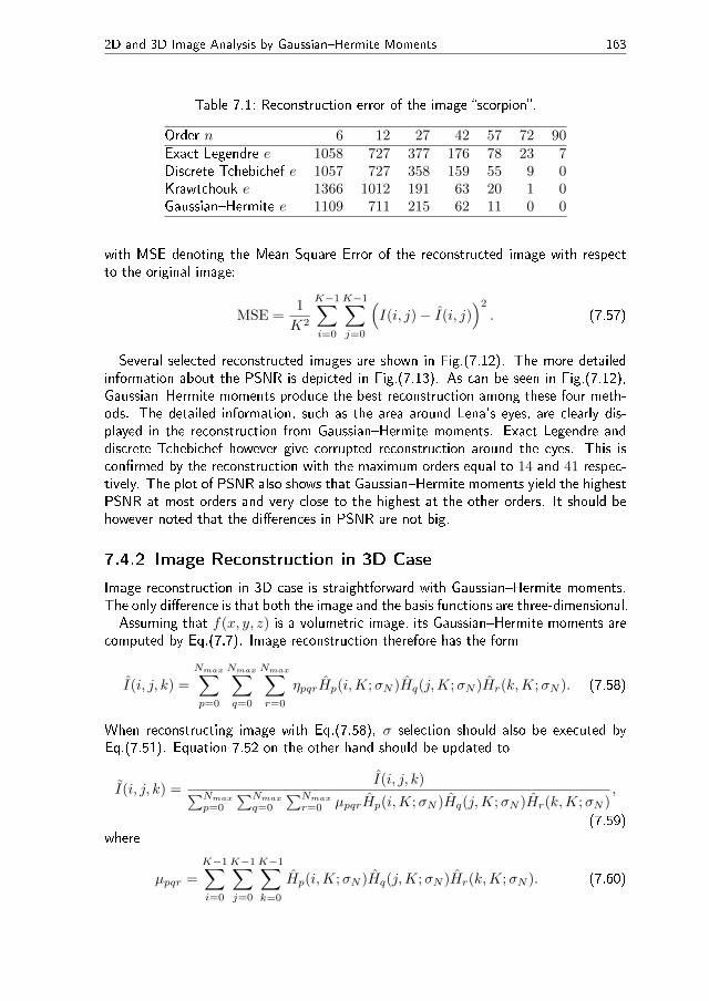
Table 7.1: Reconstruction error of the image �scorpion�.

Order n 6 12 27 42 57 72 90Exact Legendre e 1058 727 377 176 78 23 7Discrete Tchebichef e 1057 727 358 159 55 9 0Krawtchouk e 1366 1012 191 63 20 1 0Gaussian�Hermite e 1109 711 215 62 11 0 0

with MSE denoting the Mean Square Error of the reconstructed image with respectto the original image:

MSE =1

K2

K−1∑

i=0

K−1∑

j=0

(I(i, j)− I(i, j)

)2. (7.57)

Several selected reconstructed images are shown in Fig.(7.12). The more detailedinformation about the PSNR is depicted in Fig.(7.13). As can be seen in Fig.(7.12),Gaussian�Hermite moments produce the best reconstruction among these four meth-ods. The detailed information, such as the area around Lena's eyes, are clearly dis-played in the reconstruction from Gaussian�Hermite moments. Exact Legendre anddiscrete Tchebichef however give corrupted reconstruction around the eyes. This iscon�rmed by the reconstruction with the maximum orders equal to 14 and 41 respec-tively. The plot of PSNR also shows that Gaussian�Hermite moments yield the highestPSNR at most orders and very close to the highest at the other orders. It should behowever noted that the di�erences in PSNR are not big.

7.4.2 Image Reconstruction in 3D Case

Image reconstruction in 3D case is straightforward with Gaussian�Hermite moments.The only di�erence is that both the image and the basis functions are three-dimensional.Assuming that f(x, y, z) is a volumetric image, its Gaussian�Hermite moments are

computed by Eq.(7.7). Image reconstruction therefore has the form

I(i, j, k) =

Nmax∑

p=0

Nmax∑

q=0

Nmax∑

r=0

ηpqrHp(i,K;σN )Hq(j,K;σN )Hr(k,K;σN ). (7.58)

When reconstructing image with Eq.(7.58), σ selection should also be executed byEq.(7.51). Equation 7.52 on the other hand should be updated to

I(i, j, k) =I(i, j, k)

∑Nmax

p=0

∑Nmax

q=0

∑Nmax

r=0 µpqrHp(i,K;σN )Hq(j,K;σN )Hr(k,K;σN ),

(7.59)where

µpqr =

K−1∑

i=0

K−1∑

j=0

K−1∑

k=0

Hp(i,K;σN )Hq(j,K;σN )Hr(k,K;σN ). (7.60)

164 B. Yang et al.

Figure 7.12: Image reconstruction of the gray-level image �Lena� of size 100 × 100pixels. From left to right, the maximum indices of the moments are(14, 14), (41, 41), (68, 68) and (95, 95). From top to the bottom, theexact Legendre, discrete Tchebichef, Krawtchouk and Gaussian�Hermitemoments were used.


0 10 20 30 40 50 60 70 80 90 1005

10

15

20

25

30

35

40

Maximum order for reconstruction

PS

NR

Exact LegendreDiscrete TchebichefKrawtchoukGaussian−Hermite

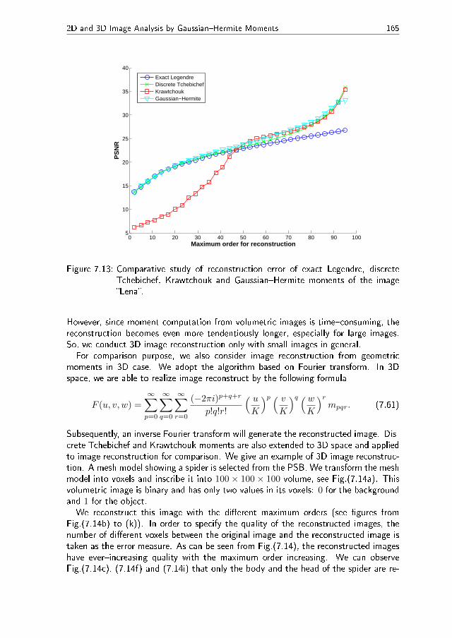
Figure 7.13: Comparative study of reconstruction error of exact Legendre, discreteTchebichef, Krawtchouk and Gaussian�Hermite moments of the image�Lena�.

However, since moment computation from volumetric images is time�consuming, thereconstruction becomes even more tendentiously longer, especially for large images.So, we conduct 3D image reconstruction only with small images in general.For comparison purpose, we also consider image reconstruction from geometric

moments in 3D case. We adopt the algorithm based on Fourier transform. In 3Dspace, we are able to realize image reconstruct by the following formula

F (u, v, w) =

∞∑

p=0

∞∑

q=0

∞∑

r=0

(−2πi)p+q+r

p!q!r!

( uK

)p ( vK

)q (wK

)rmpqr. (7.61)

Subsequently, an inverse Fourier transform will generate the reconstructed image. Dis-crete Tchebichef and Krawtchouk moments are also extended to 3D space and appliedto image reconstruction for comparison. We give an example of 3D image reconstruc-tion. A mesh model showing a spider is selected from the PSB. We transform the meshmodel into voxels and inscribe it into 100× 100× 100 volume, see Fig.(7.14a). Thisvolumetric image is binary and has only two values in its voxels: 0 for the backgroundand 1 for the object.We reconstruct this image with the di�erent maximum orders (see �gures from

Fig.(7.14b) to (k)). In order to specify the quality of the reconstructed images, thenumber of di�erent voxels between the original image and the reconstructed image istaken as the error measure. As can be seen from Fig.(7.14), the reconstructed imageshave ever�increasing quality with the maximum order increasing. We can observeFig.(7.14c), (7.14f) and (7.14i) that only the body and the head of the spider are re-

166 B. Yang et al.

constructed with lower orders. With the maximum order increasing, Gaussian�Hermiteand Krawtchouk moments reconstruct vividly the legs; however, discrete Tchebichefmoments fail to reconstruct these parts. When the maximum order reaches to 84,Gaussian�Hermite moments can completely reconstruct the original image (with error0), which exhibits the best performance in comparison with Krawtchouk moments(with error only 17) and discrete Tchebichef moments (with error 98). The maximumachievable order of geometric moment is 84 for the image �Spider�. The computationof moments whose order is greater than 84 will result in numerical over�ow. However,even if we use the moments up to the maximum achievable order, the reconstructionis still of a poor, insu�cient quality (see Fig.(7.14b)). As a result, this experimentshows that in the 3D case, Gaussian�Hermite moments have better image representa-tion ability than geometric moments and some orthogonal moments such as discreteTchebichef and Krawtchouk moments.

7.5 Application of Gaussian�Hermite Invariants in

Image Registration

In this Section, we demonstrate the application of Gaussian�Hermite invariants (GHIs)in template matching as well as in image registration. The experiment is carried outon an aerial image in Fig.(7.15a) which was downloaded from [21]. We rotated thisimage by 30◦ clockwise and then shifted it horizontally and vertically by 30 and 40pixels, respectively. The rotated image served as our reference image. We detected100 most prominent corners, road junctions and other signi�cant points which we tookas the control point candidates (CPC). Around each CPC we took a circular templateof a diameter 51 pixels, see Fig.(7.16).

To simulate real image degradations, we blurred the original image by a simulatedatmospheric turbulence blur and then a Gaussian white noise was added. We createdtwo instances with mild and heavy noise, see Fig.(7.15b) and (7.15c). These imagesplayed the role of sensed images (i.e. images to be registered).

Our goal is to locate these 100 templates in two degraded sensed images. Thetemplate matching is carried out by two methods: Geometric invariants (GEIs) andGHIs. The feature vector is composed of 18 invariants up to the order 5. Accordingto [5], the feature vector corresponding to GEIs is

Vg =[c11, c21c12, Re(c20c

212), Im(c20c

212), Re(c30c

312), Im(c30c

312), c22,

Re(c31c212), Im(c31c

212), Re(c40c

412), Im(c40c

412), c32c23, Re(c32c12),

Im(c32c12), Re(c41c312), Im(c41c

312), Re(c50c

512), Im(c50c

512)],

(7.62)


(a) Original image (b) Order 84 error 8561

(c) Order 26 error 1333 (d) Order 46 error 1003 (e) Order 84 error 98

(f) Order 26 error 955 (g) Order 46 error 435 (h) Order 84 error 17

(i) Order 26 error 1054 (j) Order 46 error 370 (k) Order 84 error 0

Figure 7.14: The reconstruction of a volumetric image by di�erent kinds of moments.(a) The original image whose size is 100 × 100 × 100 voxels; the re-constructed images by (b) geometric moments of orders (0, 0, 0) up to(84, 84, 84), (c) (d) and (e) by discrete Tchebichef moments, (f) (g) and(h) by Krawtchouk moments. (i) (j) and (k) by Gaussian�Hermite mo-ments.

168 B. Yang et al.

(a) (b) (c)

Figure 7.15: The images used in the experiment. (a) The original aerial image. (b)The degraded image with mild noise. (c) The degraded image with heavynoise.

Figure 7.16: The reference image of the size 800× 800 pixels, which is created by 30◦

clockwise rotation of Fig.(7.15a) and then shifted 30 pixels along x axisdirection and 40 pixels along y axis direction. We selected 100 templates,four of them are displayed as examples.


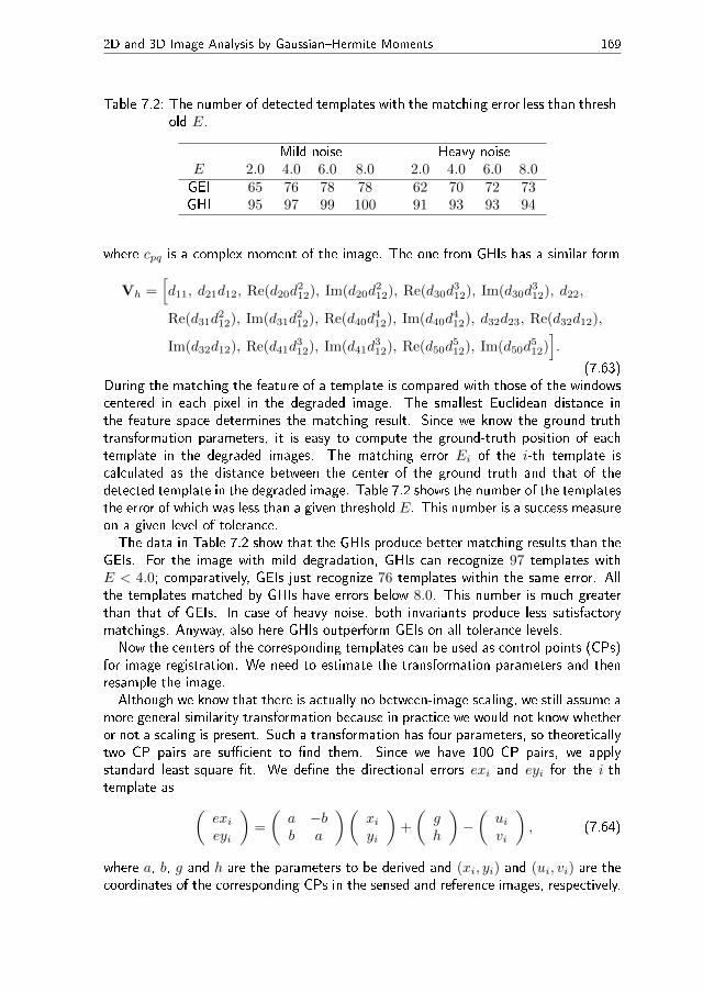
Table 7.2: The number of detected templates with the matching error less than thresh-old E.

Mild noise Heavy noiseE 2.0 4.0 6.0 8.0 2.0 4.0 6.0 8.0GEI 65 76 78 78 62 70 72 73GHI 95 97 99 100 91 93 93 94

where cpq is a complex moment of the image. The one from GHIs has a similar form

Vh =[d11, d21d12, Re(d20d

212), Im(d20d

212), Re(d30d

312), Im(d30d

312), d22,

Re(d31d212), Im(d31d

212), Re(d40d

412), Im(d40d

412), d32d23, Re(d32d12),

Im(d32d12), Re(d41d312), Im(d41d

312), Re(d50d

512), Im(d50d

512)].

(7.63)During the matching the feature of a template is compared with those of the windowscentered in each pixel in the degraded image. The smallest Euclidean distance inthe feature space determines the matching result. Since we know the ground-truthtransformation parameters, it is easy to compute the ground-truth position of eachtemplate in the degraded images. The matching error Ei of the i-th template iscalculated as the distance between the center of the ground truth and that of thedetected template in the degraded image. Table 7.2 shows the number of the templatesthe error of which was less than a given threshold E. This number is a success measureon a given level of tolerance.The data in Table 7.2 show that the GHIs produce better matching results than the

GEIs. For the image with mild degradation, GHIs can recognize 97 templates withE < 4.0; comparatively, GEIs just recognize 76 templates within the same error. Allthe templates matched by GHIs have errors below 8.0. This number is much greaterthan that of GEIs. In case of heavy noise, both invariants produce less satisfactorymatchings. Anyway, also here GHIs outperform GEIs on all tolerance levels.Now the centers of the corresponding templates can be used as control points (CPs)

for image registration. We need to estimate the transformation parameters and thenresample the image.Although we know that there is actually no between-image scaling, we still assume a

more general similarity transformation because in practice we would not know whetheror not a scaling is present. Such a transformation has four parameters, so theoreticallytwo CP pairs are su�cient to �nd them. Since we have 100 CP pairs, we applystandard least-square �t. We de�ne the directional errors exi and eyi for the i-thtemplate as

(exieyi

)=

(a −bb a

)(xiyi

)+

(gh

)−(uivi

), (7.64)

where a, b, g and h are the parameters to be derived and (xi, yi) and (ui, vi) are thecoordinates of the corresponding CPs in the sensed and reference images, respectively.

170 B. Yang et al.

The relationship between a and b on one hand and the scaling s and rotation angle αis a = s cosα and b = s sinα.We minimize a sum of error squares (N = 100 in our case)

λ =

N∑

i=1

(ex2i + ey2i ), (7.65)

which is done by setting partial derivatives of λ to zero

∂λ

∂a= 0,

∂λ

∂b= 0,

∂λ

∂g= 0,

∂λ

∂h= 0. (7.66)

Eq.(7.66) leads to a linear system of equations which directly provides the unknownparameters

∑Ni=1(x2i + y2i ) 0

∑Ni=1 xi

∑Ni=1 yi

0∑Ni=1(x2i + y2i ) −

∑Ni=1 yi

∑Ni=1 xi∑N

i=1 xi −∑Ni=1 yi N 0∑N

i=1 yi∑Ni=1 xi 0 N

×

abgh

=

∑Ni=1(xiui + yivi)∑Ni=1(xivi − yiui)∑N

i=1 ui∑Ni=1 vi

. (7.67)

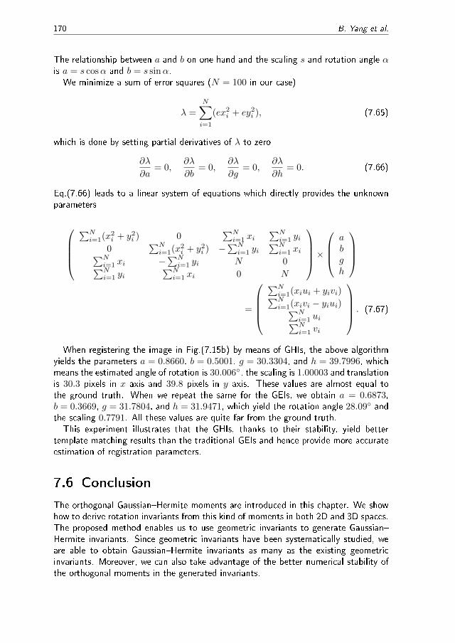
When registering the image in Fig.(7.15b) by means of GHIs, the above algorithmyields the parameters a = 0.8660, b = 0.5001, g = 30.3304, and h = 39.7996, whichmeans the estimated angle of rotation is 30.006◦, the scaling is 1.00003 and translationis 30.3 pixels in x axis and 39.8 pixels in y axis. These values are almost equal tothe ground truth. When we repeat the same for the GEIs, we obtain a = 0.6873,b = 0.3669, g = 31.7804, and h = 31.9471, which yield the rotation angle 28.09◦ andthe scaling 0.7791. All these values are quite far from the ground truth.This experiment illustrates that the GHIs, thanks to their stability, yield better

template matching results than the traditional GEIs and hence provide more accurateestimation of registration parameters.

7.6 Conclusion

The orthogonal Gaussian�Hermite moments are introduced in this chapter. We showhow to derive rotation invariants from this kind of moments in both 2D and 3D spaces.The proposed method enables us to use geometric invariants to generate Gaussian�Hermite invariants. Since geometric invariants have been systematically studied, weare able to obtain Gaussian�Hermite invariants as many as the existing geometricinvariants. Moreover, we can also take advantage of the better numerical stability ofthe orthogonal moments in the generated invariants.


The better image representation ability is also demonstrated in comparison withexact Legendre algorithm, discrete Tchebichef and Krawtchouk moments. The ex-perimental results show that Gaussian�Hermite moments outperform these popularmoments in image reconstruction. Besides, the reconstruction can also be extendedto 3D case.

The application in image registration was presented to show the potential usage ofGaussian�Hermite moments and their invariants. It indicates that Gaussian�Hermitemoments and their invariants are useful tools in image processing and pattern recog-nition and may replace the other moments used so far in many applications.

Acknowledgement

This work has been partially supported by the Czech Science Foundation under theGrant No. P103/11/1552, by the Academy of Sciences of the Czech Republic underthe program of Human Resources Support, and by the ERCIM.

References

[1] N. Canterakis. 3D Zernike moments and Zernike a�ne invariants for 3D imageanalysis and recognition. In Scandinavian Conference on Image Analysis (SCIA),pages 85�93. DSAGM, 1999.

[2] D. Cyganski and J.A. Orr. Object recognition and orientation determination bytensor methods. JAI Press, Greenwich, United Kingdom, �rst edition, 1988.

[3] J. Fehr. Local rotation invariant patch descriptors for 3D vector �elds. In Inter-national Conference on Pattern Recognition (ICPR), pages 1381�1384, August2010.

[4] J. Fehr and H. Burkhardt. 3D rotation invariant local binary patterns. In Inter-national Conference on Pattern Recognition (ICPR), pages 1�4, December 2008.

[5] J. Flusser. On the independence of rotation moment invariants. Pattern Recog-nition, 33(9):1405�1410, 2000.

[6] J. Flusser, J. Boldys, and B. Zitova. Moment forms invariant to rotation andblur in arbitrary number of dimensions. IEEE Transactions on Pattern Analysisand Machine Intelligence, 25(2):234�246, 2003.

[7] J. Flusser, T. Suk, and B. Zitova. Moments and Moment Invariants in PatternRecognition. Wiley, Chichester, United Kingdom, 2009.

[8] J.M. Galvez and M. Canton. Normalization and shape recognition of three-dimensional objects by 3D moments. Pattern Recognition, 26(5):667�681, 1993.

[9] X. Guo. Three dimensional moment invariants under rigid transformation. InInternational Conference on Computer Analysis of Images and Patterns (CAIP),volume 719 of LNCS, pages 518�522, Budapest, Hungary, 1993.

[10] K. M. Hosny. New set of rotationally Legendre moment invariants. InternationalJournal of Electrical and Electronics Engineering, 4(3):176�180, 2010.

[11] K.M. Hosny. Exact Legendre moment computation for gray level images. PatternRecognition, 40(12):3597�3605, 2007.

172 B. Yang et al.

[12] M.K. Hu. Visual pattern recognition by moment invariants. IRE Transactions onInformation Theory, 8(2):179�187, 1962.

[13] R. Kakarala and D. Mao. A theory of phase-sensitive rotation invariance withspherical harmonic and moment-based representations. In IEEE Conference onComputer Vision and Pattern Recognition (CVPR), pages 105�112, June 2010.

[14] M. Kazhdan. An approximate and e�cient method for optimal rotation alignmentof 3D models. IEEE Transactions on Pattern Analysis and Machine Intelligence,29(7):1221�1229, 2007.

[15] M. Kazhdan, T. Funkhouser, and S. Rusinkiewicz. Rotation invariant sphericalharmonic representation of 3D shape descriptors. In Eurographics/ACM SIG-GRAPH symposium on Geometry processing (SGP), pages 156�164, Aire-la-Ville,Switzerland, June 2003. Eurographics Association.

[16] A. Khotanzad and Y.H. Hong. Invariant image recognition by Zernike moments.IEEE Transactions on Pattern Analysis and Machine Intelligence, 12(5):489�497,1990.

[17] Y.J. Li. Reforming the theory of invariant moments for pattern recognition.Pattern Recognition, 25(7):723�730, 1992.

[18] C.H. Lo and H.S. Don. 3-D moment forms: Their construction and applicationto object identi�cation and positioning. IEEE Transactions on Pattern Analysisand Machine Intelligence, 11(10):1053�1064, 1989.

[19] J.F. Mangin, F. Poupon, E. Duchesnay, D. Riviere, A. Cachia, D.L. Collins, A.C.Evans, and J. Regis. Brain morphometry using 3D moment invariants. MedicalImage Analysis, 8(3):187�196, 2004.

[20] R. Mukundan. Some computational sspects of discrete orthonormal moments.IEEE Transactions on Image Processing, 13(8):1055�1059, 2004.

[21] County Orange. Aerial image sample, 2012. [online] - Available:http://www.co.orange.nc.us/soilwater/AerialPhotos.asp.

[22] Princeton. Princeton Shape Benchmark, 2013. [online] - Available:http://shape.cs.princeton.edu/benchmark/.

[23] T.H. Reiss. Recognizing planar objects using invariant image features. Springer-Verlag, Berlin, Germany, �rst edition, 1993.

[24] F A. Sadjadi and E.L. Hall. Three-Dimensional moment invariants. IEEE Trans-actions on Pattern Analysis and Machine Intelligence, PAMI-2(2):127�136, 1980.

[25] H. Skibbe, M. Reisert, and H. Burkhardt. SHOG-Spherical HOG descriptors forrotation invariant 3D object detection. In R. Mester and M. Felsberg, editors,Deutsche Arbeitsgemeinschaft für Mustererkennung (DAGM), volume 6835 ofLNCS, pages 142�151. Springer Berlin Heidelberg, 2011.

[26] T. Suk and J. Flusser. Tensor method for constructing 3D moment invariants. InInternational Conference on Computer Analysis of Images and Patterns (CAIP),volume 6855 of LNCS, pages 212�219, Seville,Spanien, 2011.

[27] T. Suk and J. Flusser. 3D rotation invariants, 2012. [online] - Available:http://zoi.utia.cas.cz/3DRotationInvariants.

[28] M. Trummer, H. Suesse, and J. Denzler. Coarse registration of 3D surface trian-gulations based on moment invariants with applications to object alignment andidenti�cation. In International Conference on Computer Vision (ICCV), pages1273�1279, October 2009.


[29] A. Wallin and O. Kubler. Complete sets of complex Zernike moment invariantsand the role of the pseudoinvariants. IEEE Transactions on Pattern Analysis andMachine Intelligence, 17(11):1106�1110, 1995.

[30] Wikipedia. Euler angles, 2012. [online] - Available:http://en.wikipedia.org/wiki/Euler_angles.

[31] W.H. Wong, W.C. Siu, and K.M. Lam. Generation of moment invariants andtheir uses for character recognition. Pattern Recognition Letters, 16(2):115�123,1995.

[32] D. Xu and H. Li. Geometric moment invariants. Pattern Recognition, 41(1):240�249, 2008.

[33] B. Yang and M. Dai. Image analysis by Gaussian�Hermite moments. SignalProcessing, 91(10):2290�2303, 2011.

[34] B. Yang and M. Dai. Image reconstruction from continuous Gaussian�Hermitemoments implemented by discrete algorithm. Pattern Recognition, 45:1602�1616,2012.

[35] B. Yang, J. Flusser, and T. Suk. 3D rotation invariants of Gaussian�Hermitemoments. submitted to Pattern Recognition Letters.

[36] B. Yang, G. Li, H. Zhang, and M. Dai. Rotation and translation invariantsof Gaussian�Hermite moments. Pattern Recognition Letters, 32(9):1283�1298,2011.

[37] P.T. Yap, R. Paramesran, and S.H. Ong. Image analysis by Krawtchouk moments.IEEE Transactions on Image Processing, 12(11):1367�1377, 2003.

Documents

Chapter 7: 2D and 3D Image Analysis by Gaussian–Hermite ...library.utia.cas.cz/separaty/2014/ZOI/flusser-0429813.pdf · 2D and 3D Image Analysis by Gaussian Hermite Moments 145