Chapter 7. COMPLETELY RANDOMIZED DESIGN WITH AND WITHOUT SUBSAMPLES

Responses among experimental units vary due to many different causes, known and unknown. The process of the separation and comparison of sources of variation is called the Analysis of Variance (AOV). The process is more general than the t-test as any number of treatment means can be simultaneously compared. The sugar beet experiment discussed in Chapter 5 and 6 involved six rates of nitrogen fertilizer. Table 7-1 gives root yield data for the five replications of all six treatments.

Table 7-1. Root yields (tons/acre) of plots fertilized with six levels of nitrogen.

Treatment (lb. /acre)

Replications Total (Yi.)

Mean ( ).Yi

A(0) 31.3 33.4 29.2 32.2 33.9 160.0 32.00

B(50) 38.8 37.5 37.4 35.8 38.4 187.9 37.58

C(100) 40.9 39.2 39.5 38.6 39.8 198.0 39.60

D(150) 40.9 41.7 39.4 40.1 40.0 202.1 40.42

E(200) 39.7 40.6 39.2 38.7 41.9 200.1 40.02

F(250) 40.6 41.0 41.5 41.1 39.8 204.0 40.80

Overall 1152.1 38.40

In this case, the experimenter may want to compare the six treatment means simultaneously to decide if there is any difference among treatments. The AOV can be used for this purpose. It involves:

1. The partitioning of the total sum of squares of the experiment into each specified source of variation.

2. The estimation of the variance per experimental unit from these sources of variation.

3. The comparison of these variances by F-tests, which will lead to conclusions concerning the

equality of the means. For the experiment in Table 7-1, the total sum of squares for root yield can be separated into a sum of squares representing variability among treatment means (a between treatment sum of squares) and a sum of squares resulting from random variation among plots within treatments (within treatment sum of squares). Each sum of squares divided by its appropriate df results in a mean square. The within treatment mean square measures the random variability among experimental units, an estimate of the population variance, σ2. If there are no treatment effects, the between treatment mean square is also an estimate of σ2. The ratio of between treatment mean square divided by within treatment mean square provides an F-test of the equality of treatment means. Experiments must be designed to provide valid estimates of the population variance from various classifications of the experimental units. A principal feature of experimental design is the way in which experimental units are grouped, for example into treatments, blocks, locations, litters, years, etc., so that mean squares can be obtained for each source of variation. The exact form of the AOV therefore

depends on the design used for the experiment. In chapters that follow, the AOV will be developed in the context of several designs. Certain assumptions must be satisfied for an appropriate use of the AOV. These are: 1) Measurements made on experimental units within a classification are normally distributed. For data in Table 7-1, this means that root yields within the treatments are normally distributed. 2) An observation made on one experimental unit is independent from any other experimental unit. That is the root yield from one plot is not influenced by any other plot. 3) The variances of different samples are homogeneous, i.e., each treatment variance estimates the same population variance. 4) Treatment and environmental effects are additive. 7.1 Completely Randomized Design Without Subsamples As the name implies, the completely randomized design (CRD) refers to the random assignment of experimental units to a set of treatments. It is essential to have more than one experimental unit per treatment to estimate the magnitude of experimental error and to make probability statements concerning treatment effects. Randomization To illustrate the procedure for the random assignment of experimental units to treatments, we will show how the treatments of Table 7-1 might have been assigned to the 30 experimental units (plots of land) of that experiment.

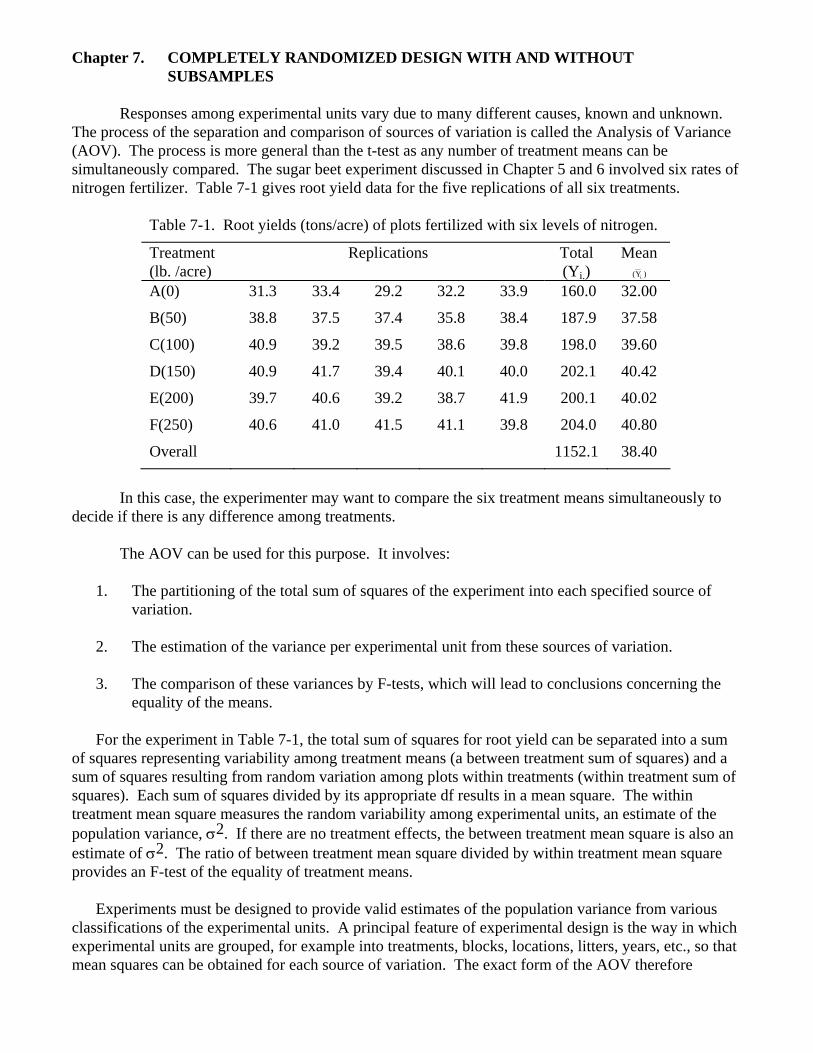
1. Arbitrarily number the experimental units (top left number in each plot of Figure 7-1).

2. Refer to a table of random numbers (Appendix Table A-1). Note that some of our experimental units are two-digit numbers. Therefore we must use two lines or columns of the random number table. Start at some arbitrary point -- say we will read down columns 7 and 8 of Appendix Table A-1 and record the two digit numbers as we go, skipping those previously recorded, until we have a random number for each experimental unit (the number in the top middle of each plot of Figure 7-1).

3. Rank the random numbers (top right number in each lot of Figure 7-1).

4. Assign each treatment in order (A through F) to plots according to the necessary ranks, to give

as many replications as needed for each treatment. In this case, we want five replications per treatment.

1-58-18 D(0.9)

7-96-29 F(41.0)

13-64-21 E(39.2)

19-20-07 B(37.5)

25-25-08 B(38.4)

2-97-30 F(40.6)

8-51-15 C(39.5)

14-52-16 D(41.7)

20-73-23 E(38.7)

26-60-19 D(40.1)

3-42-11 C(40.9)

9-74-24 E(39.7)

15-62-20 D(39.4)

21-44-12 C(39.8)

27-95-28 F(39.8)

4-07-02 A(31.3)

10-79-25 E(40.6)

16-28-09 B(38.8)

22-01-01 A(32.2)

28-15-04 A(33.9)

5-49-14 D(39.2)

11-13-03 A(29.2)

17-92-27 F(41.1)

23-31-10 B(37.4)

29-53-17 D(40.0)

6-14-05 A(33.4)

12-85-26 F(41.5)

18-45-13 C(38.6)

24-17-06 B(35.8)

30-65-22 E(41.9)

Figure 7-1. Thirty sugar beet plots numbered in sequence; randomly assigned two digit numbers

from Appendix Table A-1 (top middle); a ranking of the random number (top right); the assignment treatment (A through F); and resulting root yields (parentheses). See Table 7-1 for the root yields organized by treatments.

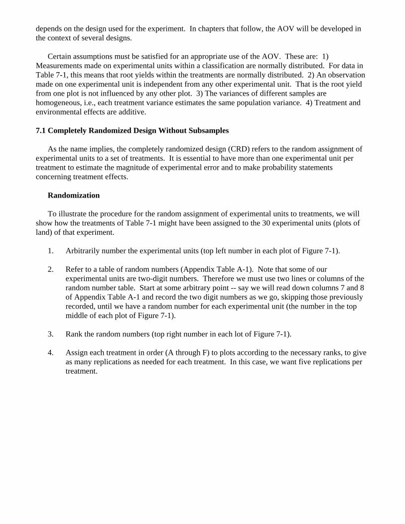
Analysis of Variance The null hypothesis to be tested is:

H0: μ1 = μ2 = ... = μk for k treatments The procedure for testing this hypothesis results in the construction and completion of an AOV table (Table 7-2). Note that there are only two sources of variation in the CRD, between and within treatments and that the total df in the experiment are partitioned into these two sources.

Table 7-2. Analysis of variance of a CRD. Source

df

Sum of squares (SS)

Mean squares (MS)

Observed F

Total kr - 1 TSS

Between treatments k - 1 SST MST MST/MSE

Within treatments (experimental error)

k(r - 1) SSE MSE

where r is the replication number per treatment. Table 7-3 is the completed AOV for the experiment of Figure 7-1.

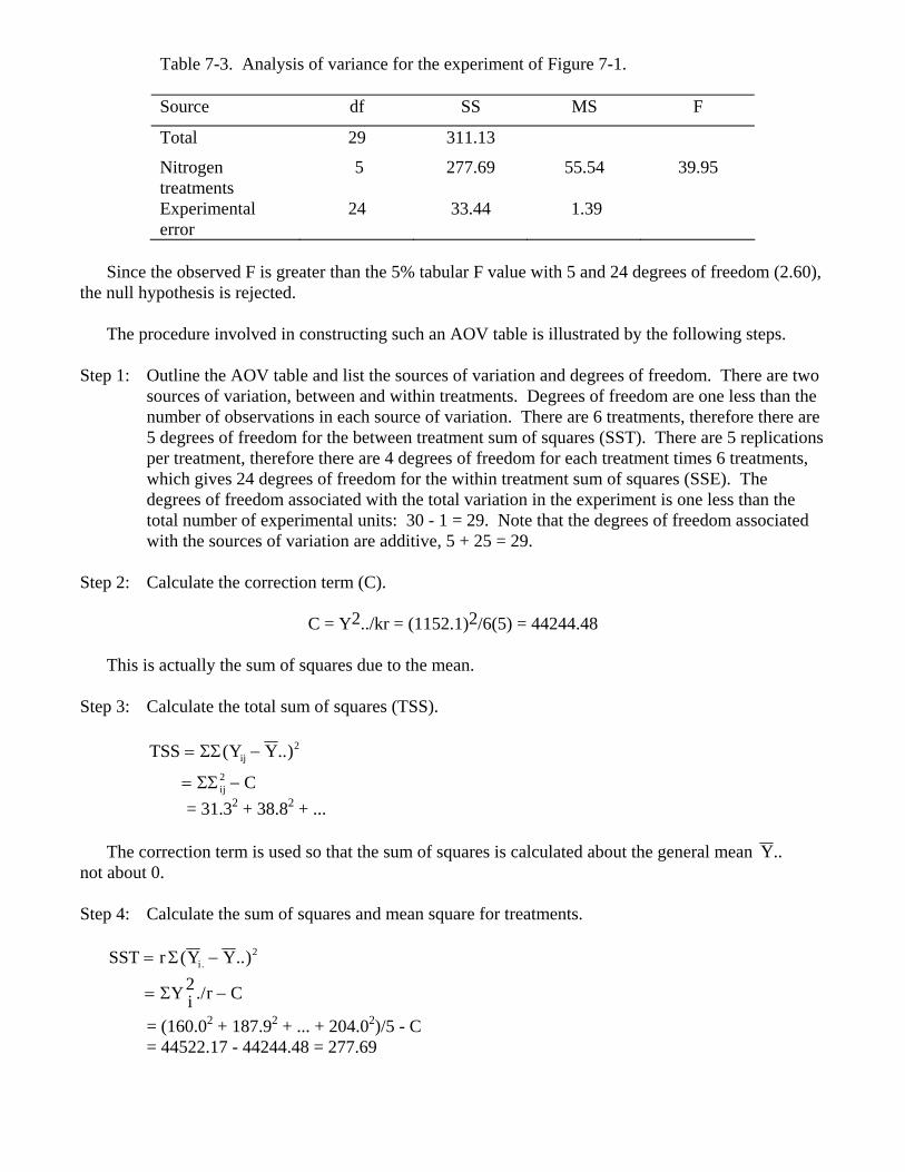
Table 7-3. Analysis of variance for the experiment of Figure 7-1. Source df SS MS F

Total 29 311.13

Nitrogen treatments

5 277.69 55.54 39.95

Experimental error

24 33.44 1.39

Since the observed F is greater than the 5% tabular F value with 5 and 24 degrees of freedom (2.60), the null hypothesis is rejected. The procedure involved in constructing such an AOV table is illustrated by the following steps. Step 1: Outline the AOV table and list the sources of variation and degrees of freedom. There are two

sources of variation, between and within treatments. Degrees of freedom are one less than the number of observations in each source of variation. There are 6 treatments, therefore there are 5 degrees of freedom for the between treatment sum of squares (SST). There are 5 replications per treatment, therefore there are 4 degrees of freedom for each treatment times 6 treatments, which gives 24 degrees of freedom for the within treatment sum of squares (SSE). The degrees of freedom associated with the total variation in the experiment is one less than the total number of experimental units: 30 - 1 = 29. Note that the degrees of freedom associated with the sources of variation are additive, 5 + 25 = 29.

Step 2: Calculate the correction term (C).

C = Y2../kr = (1152.1)2/6(5) = 44244.48 This is actually the sum of squares due to the mean. Step 3: Calculate the total sum of squares (TSS).

TSS Y Y

Cij

ij

= −

= −

ΣΣ

ΣΣ

( . 2

2

.)

= 31.32 + 38.82 + ... The correction term is used so that the sum of squares is calculated about the general mean Y.. not about 0. Step 4: Calculate the sum of squares and mean square for treatments.

SST r Y Y

Y i r C

i= −

= −

Σ

Σ

( .

./

.2

2.)

= (160.02 + 187.92 + ... + 204.02)/5 - C = 44522.17 - 44244.48 = 277.69

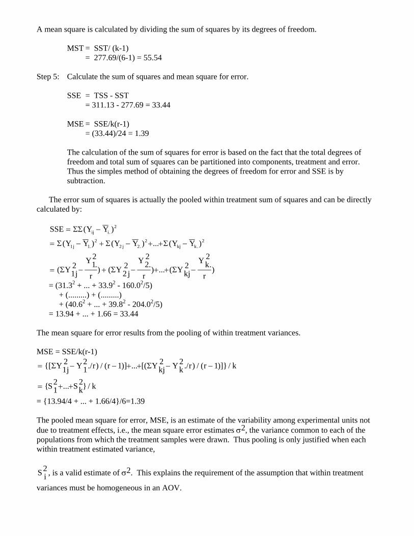
A mean square is calculated by dividing the sum of squares by its degrees of freedom. MST = SST/ (k-1) = 277.69/(6-1) = 55.54 Step 5: Calculate the sum of squares and mean square for error. SSE = TSS - SST = 311.13 - 277.69 = 33.44 MSE = SSE/k(r-1) = (33.44)/24 = 1.39 The calculation of the sum of squares for error is based on the fact that the total degrees of

freedom and total sum of squares can be partitioned into components, treatment and error. Thus the simples method of obtaining the degrees of freedom for error and SSE is by subtraction.

The error sum of squares is actually the pooled within treatment sum of squares and can be directly calculated by:

SSE Y Y

Y Y Y Y Y Y

Y jY

rY j

Y

rYkj

Ykr

ij i

j j kj

= −

= − + − + + −

= − + − + + −

ΣΣ

Σ Σ Σ

Σ Σ Σ

( )

( ) ( ) ... ( )

( .) ( .) ... ( .)

.

. .

2

1 12

2 22 2

21

21 2

2

22 2

2k.

k

= (31.32 + ... + 33.92 - 160.02/5) + (.........) + (.........) + (40.62 + ... + 39.82 - 204.02/5) = 13.94 + ... + 1.66 = 33.44 The mean square for error results from the pooling of within treatment variances. MSE = SSE/k(r-1)

= − − + + − −

= + +

{[ ./ ) / ( )] ... [( ./ ) / ( )]} /

{ ... } /

Σ ΣY j Y r r Ykj Yk r r

S Sk k

21

21 1 2 2 1

21

2

= {13.94/4 + ... + 1.66/4}/6=1.39 The pooled mean square for error, MSE, is an estimate of the variability among experimental units not due to treatment effects, i.e., the mean square error estimates σ2, the variance common to each of the populations from which the treatment samples were drawn. Thus pooling is only justified when each within treatment estimated variance,

S i2 , is a valid estimate of σ2. This explains the requirement of the assumption that within treatment

variances must be homogeneous in an AOV.

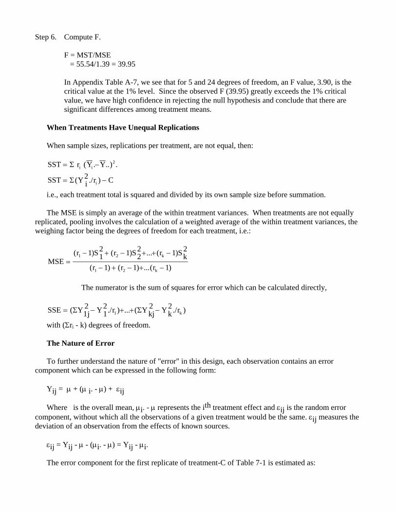
Step 6. Compute F. F = MST/MSE = 55.54/1.39 = 39.95 In Appendix Table A-7, we see that for 5 and 24 degrees of freedom, an F value, 3.90, is the

critical value at the 1% level. Since the observed F (39.95) greatly exceeds the 1% critical value, we have high confidence in rejecting the null hypothesis and conclude that there are significant differences among treatment means.

When Treatments Have Unequal Replications When sample sizes, replications per treatment, are not equal, then:

SST r Y Y

SST Y i r C

i i

i

= −

= −

Σ

Σ

( . ..)

( ./ )

2

2.

i.e., each treatment total is squared and divided by its own sample size before summation. The MSE is simply an average of the within treatment variances. When treatments are not equally replicated, pooling involves the calculation of a weighted average of the within treatment variances, the weighing factor being the degrees of freedom for each treatment, i.e.:

MSEr S r S r Sk

r r r

k

k

=− + − + + −

− + − + −

( ) ( ) ... ( )

( ) ( ) ...( )

1 2

1 2

1 21 1 2

2 1 2

1 1 1

The numerator is the sum of squares for error which can be calculated directly,

SSE Y j Y r Ykj Yk rk= − + + −( ./ ) ... ( ./ )Σ Σ21

21

2 21

with (Σri - k) degrees of freedom. The Nature of Error To further understand the nature of "error" in this design, each observation contains an error component which can be expressed in the following form: Yij = μ + (μ i. - μ) + εij Where is the overall mean, μi. - μ represents the ith treatment effect and εij is the random error component, without which all the observations of a given treatment would be the same. εij measures the deviation of an observation from the effects of known sources. εij = Yij - μ - (μi. - μ) = Yij - μi. The error component for the first replicate of treatment-C of Table 7-1 is estimated as:

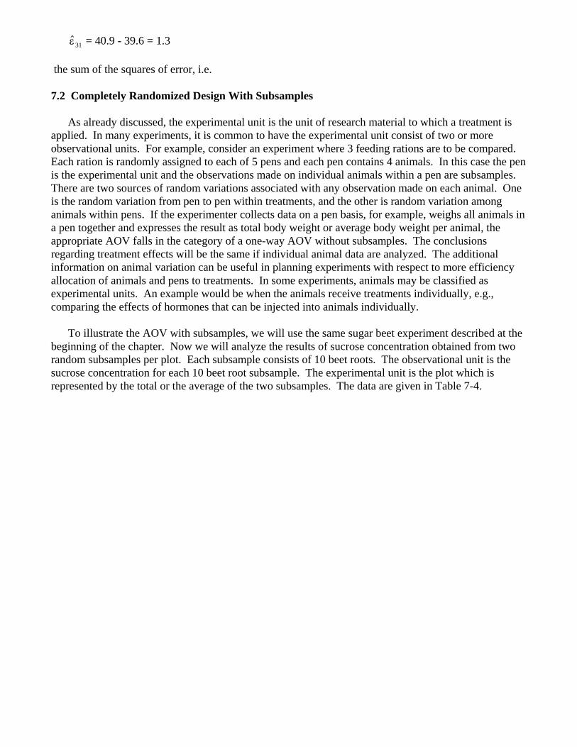
= 40.9 - 39.6 = 1.3 $ε31

the sum of the squares of error, i.e. 7.2 Completely Randomized Design With Subsamples As already discussed, the experimental unit is the unit of research material to which a treatment is applied. In many experiments, it is common to have the experimental unit consist of two or more observational units. For example, consider an experiment where 3 feeding rations are to be compared. Each ration is randomly assigned to each of 5 pens and each pen contains 4 animals. In this case the pen is the experimental unit and the observations made on individual animals within a pen are subsamples. There are two sources of random variations associated with any observation made on each animal. One is the random variation from pen to pen within treatments, and the other is random variation among animals within pens. If the experimenter collects data on a pen basis, for example, weighs all animals in a pen together and expresses the result as total body weight or average body weight per animal, the appropriate AOV falls in the category of a one-way AOV without subsamples. The conclusions regarding treatment effects will be the same if individual animal data are analyzed. The additional information on animal variation can be useful in planning experiments with respect to more efficiency allocation of animals and pens to treatments. In some experiments, animals may be classified as experimental units. An example would be when the animals receive treatments individually, e.g., comparing the effects of hormones that can be injected into animals individually. To illustrate the AOV with subsamples, we will use the same sugar beet experiment described at the beginning of the chapter. Now we will analyze the results of sucrose concentration obtained from two random subsamples per plot. Each subsample consists of 10 beet roots. The observational unit is the sucrose concentration for each 10 beet root subsample. The experimental unit is the plot which is represented by the total or the average of the two subsamples. The data are given in Table 7-4.

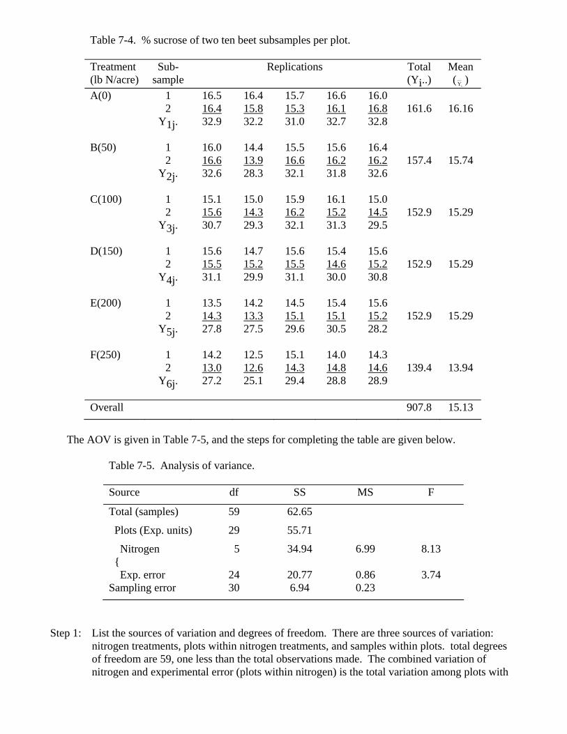
Table 7-4. % sucrose of two ten beet subsamples per plot. Treatment (lb N/acre)

Sub- sample

Replications Total (Yi..)

Mean (Yi. .

) A(0)

1 2

Y1j.

16.5 16.432.9

16.4 15.832.2

15.7 15.331.0

16.6 16.132.7

16.0 16.832.8

161.6

16.16

B(50) 1 2

Y2j.

16.0 16.632.6

14.4 13.928.3

15.5 16.632.1

15.6 16.231.8

16.4 16.232.6

157.4

15.74

C(100) 1 2

Y3j.

15.1 15.630.7

15.0 14.329.3

15.9 16.232.1

16.1 15.231.3

15.0 14.529.5

152.9

15.29

D(150) 1 2

Y4j.

15.6 15.531.1

14.7 15.229.9

15.6 15.531.1

15.4 14.630.0

15.6 15.230.8

152.9

15.29

E(200) 1 2

Y5j.

13.5 14.327.8

14.2 13.327.5

14.5 15.129.6

15.4 15.130.5

15.6 15.228.2

152.9

15.29

F(250) 1 2

Y6j.

14.2 13.027.2

12.5 12.625.1

15.1 14.329.4

14.0 14.828.8

14.3 14.628.9

139.4

13.94

Overall 907.8 15.13

The AOV is given in Table 7-5, and the steps for completing the table are given below.

Table 7-5. Analysis of variance. Source df SS MS F

Total (samples) 59 62.65

Plots (Exp. units) 29 55.71

Nitrogen { Exp. error

5

24

34.94

6.99

0.86

8.13

20.77 3.74 Sampling error 30 6.94 0.23

Step 1: List the sources of variation and degrees of freedom. There are three sources of variation:

nitrogen treatments, plots within nitrogen treatments, and samples within plots. total degrees of freedom are 59, one less than the total observations made. The combined variation of nitrogen and experimental error (plots within nitrogen) is the total variation among plots with

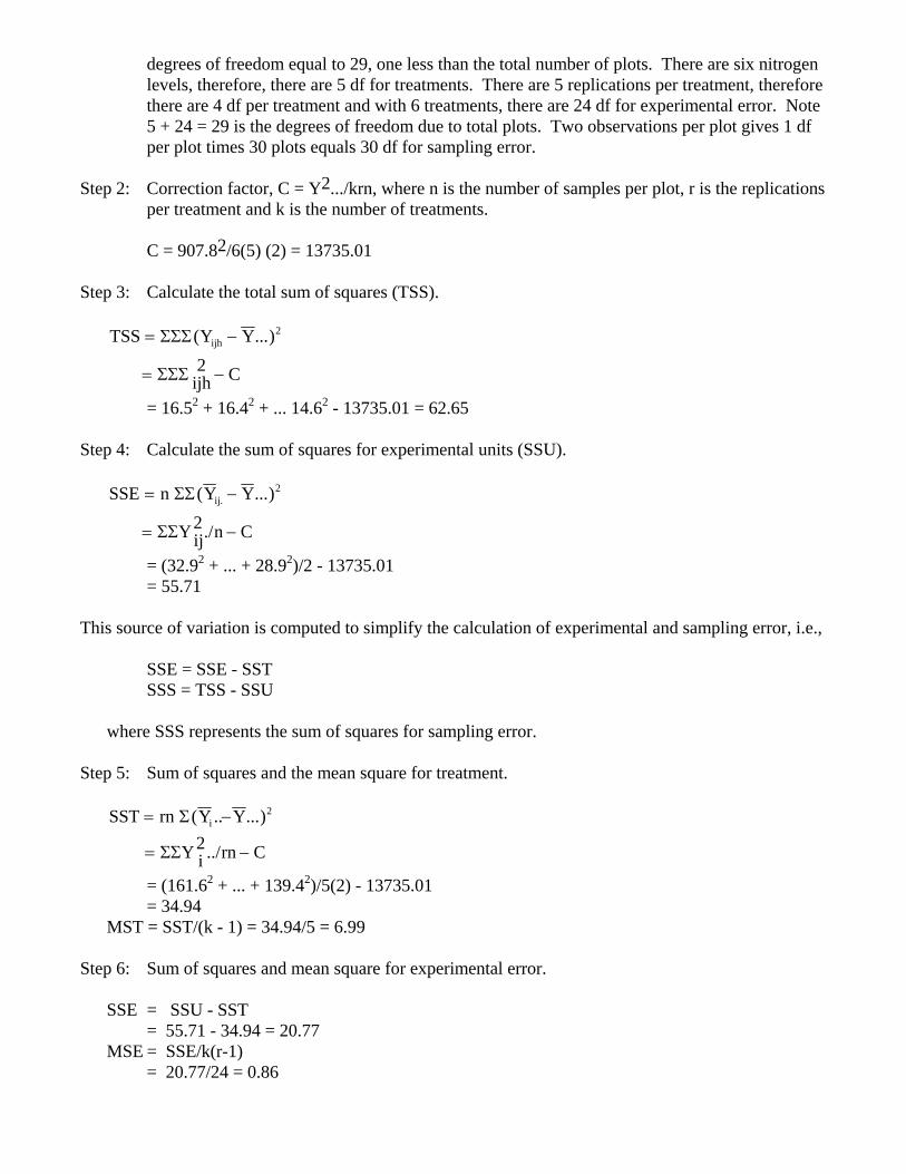
degrees of freedom equal to 29, one less than the total number of plots. There are six nitrogen levels, therefore, there are 5 df for treatments. There are 5 replications per treatment, therefore there are 4 df per treatment and with 6 treatments, there are 24 df for experimental error. Note 5 + 24 = 29 is the degrees of freedom due to total plots. Two observations per plot gives 1 df per plot times 30 plots equals 30 df for sampling error.

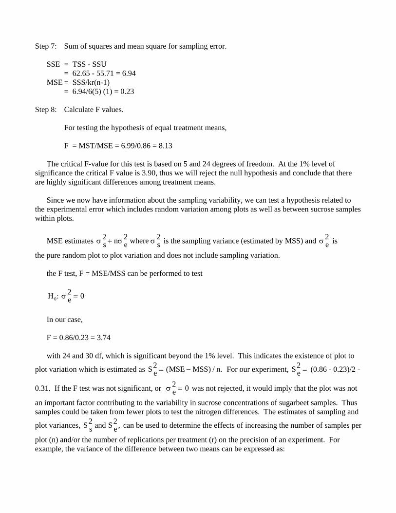
Step 2: Correction factor, C = Y2.../krn, where n is the number of samples per plot, r is the replications

per treatment and k is the number of treatments. C = 907.82/6(5) (2) = 13735.01 Step 3: Calculate the total sum of squares (TSS).

TSS Y Y

ijh C

ijh= −

= −

ΣΣΣ

ΣΣΣ

( ...)2

2

= 16.52 + 16.42 + ... 14.62 - 13735.01 = 62.65 Step 4: Calculate the sum of squares for experimental units (SSU).

SSE n Y Y

Yij n C

ij= −

= −

ΣΣ

ΣΣ

( ..

./

.2

2.)

= (32.92 + ... + 28.92)/2 - 13735.01 = 55.71 This source of variation is computed to simplify the calculation of experimental and sampling error, i.e., SSE = SSE - SST SSS = TSS - SSU where SSS represents the sum of squares for sampling error. Step 5: Sum of squares and the mean square for treatment.

SST rn Y Y

Y i rn C

i= −

= −

Σ

ΣΣ

( .. ...)

../

2

2

= (161.62 + ... + 139.42)/5(2) - 13735.01 = 34.94 MST = SST/(k - 1) = 34.94/5 = 6.99 Step 6: Sum of squares and mean square for experimental error. SSE = SSU - SST = 55.71 - 34.94 = 20.77 MSE = SSE/k(r-1) = 20.77/24 = 0.86

Step 7: Sum of squares and mean square for sampling error. SSE = TSS - SSU = 62.65 - 55.71 = 6.94 MSE = SSS/kr(n-1) = 6.94/6(5) (1) = 0.23 Step 8: Calculate F values. For testing the hypothesis of equal treatment means, F = MST/MSE = 6.99/0.86 = 8.13 The critical F-value for this test is based on 5 and 24 degrees of freedom. At the 1% level of significance the critical F value is 3.90, thus we will reject the null hypothesis and conclude that there are highly significant differences among treatment means. Since we now have information about the sampling variability, we can test a hypothesis related to the experimental error which includes random variation among plots as well as between sucrose samples within plots.

MSE estimates σ σ is the sampling variance (estimated by MSS) and σ is σ2 2s n e where s+ 2

) / .

2

2e

the pure random plot to plot variation and does not include sampling variation. the F test, F = MSE/MSS can be performed to test

H e02 0: σ =

In our case, F = 0.86/0.23 = 3.74 with 24 and 30 df, which is significant beyond the 1% level. This indicates the existence of plot to

plot variation which is estimated as For our experiment, (0.86 - 0.23)/2 -

0.31. If the F test was not significant, or was not rejected, it would imply that the plot was not

an important factor contributing to the variability in sucrose concentrations of sugarbeet samples. Thus samples could be taken from fewer plots to test the nitrogen differences. The estimates of sampling and

plot variances, S can be used to determine the effects of increasing the number of samples per

plot (n) and/or the number of replications per treatment (r) on the precision of an experiment. For example, the variance of the difference between two means can be expressed as:

S e MSE MSS n2 = −( S e2 =

σ2 0e =

s and S e2 ,

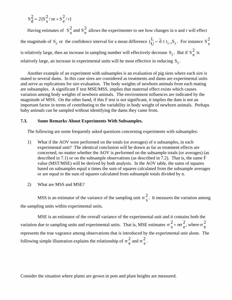
Sd S s nr S e r2 2 2 2= +{ / / }

2

Having estimates of S allows the experimenter to see how changes in n and r will effect

the magnitude of

s and S e2

Sd or the confidence interval for a mean difference ( /LU d t Sd= ± α 2 . For instance

is relatively large, then an increase in sampling number will effectively decrease

S s2

Sd . But if S is

relatively large, an increase in experimental units will be most effective in reducing e2

Sd . Another example of an experiment with subsamples is an evaluation of pig sires where each sire is mated to several dams. In this case sires are considered as treatments and dams are experimental units and serve as replications for sire evaluation. The body weights of newborn animals from each mating are subsamples. A significant F test MSE/MSS, implies that maternal effect exists which causes variation among body weights of newborn animals. The environment influences are indicated by the magnitude of MSS. On the other hand, if this F test is not significant, it implies the dam is not an important factor in terms of contributing to the variability in body weight of newborn animals. Perhaps baby animals can be sampled without identifying the dams they came from. 7.3. Some Remarks About Experiments With Subsamples. The following are some frequently asked questions concerning experiments with subsamples: 1) What if the AOV were performed on the totals (or averages) of n subsamples, in each

experimental unit? The identical conclusion will be drawn as far as treatment effects are concerned, no matter whether the AOV is performed on the subsample totals (or averages) (as described in 7.1) or on the subsample observations (as described in 7.2). That is, the same F value (MST/MSE) will be derived by both analysis. In the AOV table, the sums of squares based on subsamples equal n times the sum of squares calculated from the subsample averages or are equal to the sum of squares calculated from subsample totals divided by n.

2) What are MSS and MSE?

MSS is an estimator of the variance of the sampling unit . It measures the variation among

the sampling units within experimental units.

σ2s

MSE is an estimator of the overall variance of the experimental unit and it contains both the

variation due to sampling units and experimental units. That is, MSE estimates

represents the true vagrance among observations that is introduced by the experimental unit alone. The

following simple illustration explains the relationship of .

σ σ σ2 2s n e where e+ , 2

σ σ2 2e and s

Consider the situation where plants are grown in pots and plant heights are measured.

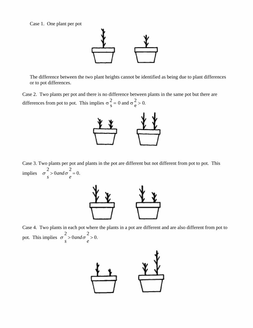
Case 1. One plant per pot

The difference between the two plant heights cannot be identified as being due to plant differences or to pot differences.

Case 2. Two plants per pot and there is no difference between plants in the same pot but there are

differences from pot to pot. This implies σ σ2 0 2 0s and e= > .

Case 3. Two plants per pot and plants in the pot are different but not different from pot to pot. This

implies .02

02

=>e

ands

σσ

Case 4. Two plants in each pot where the plants in a pot are different and are also different from pot to

pot. This implies .02

02

>>e

ands

σσ

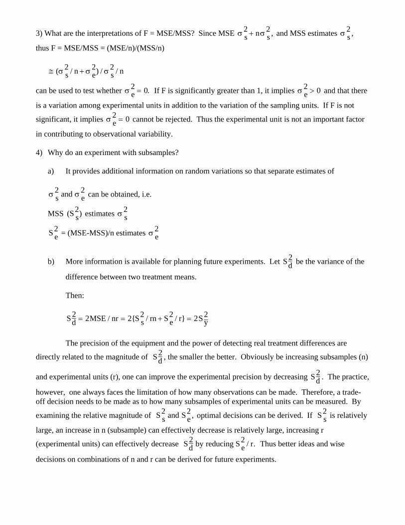
3) What are the interpretations of F = MSE/MSS? Since MSE σ and MSS estimates σ

thus F = MSE/MSS = (MSE/n)/(MSS/n)

σ2s n s+ ,2

2

)

2s ,

≅ +( / ) / /σ σ σ2 2 2s n e s n

can be used to test whether If F is significantly greater than 1, it implies and that there

is a variation among experimental units in addition to the variation of the sampling units. If F is not

significant, it implies cannot be rejected. Thus the experimental unit is not an important factor

in contributing to observational variability.

σ2 0e = . σ2 0e >

σ2 0e =

4) Why do an experiment with subsamples? a) It provides additional information on random variations so that separate estimates of

can be obtained, i.e. σ σ2s and e

MSS ( estimates S s2 σ2

s

= (MSE-MSS)/n estimates S e2 σ2

e

b) More information is available for planning future experiments. Let Sd2 be the variance of the

difference between two treatment means. Then:

Sd MSE nr S s rn S e r S y2 2 2 2 2 2 2= = + =/ { / / }

The precision of the equipment and the power of detecting real treatment differences are

directly related to the magnitude of Sd2 , the smaller the better. Obviously be increasing subsamples (n)

and experimental units (r), one can improve the experimental precision by decreasing Sd2 . The practice,

however, one always faces the limitation of how many observations can be made. Therefore, a trade-off decision needs to be made as to how many subsamples of experimental units can be measured. By

examining the relative magnitude of S optimal decisions can be derived. If is relatively

large, an increase in n (subsample) can effectively decrease is relatively large, increasing r

(experimental units) can effectively decrease

s and S e2 ,2 S s

2

Sd by reducing S e r2 2 / . Thus better ideas and wise

decisions on combinations of n and r can be derived for future experiments.

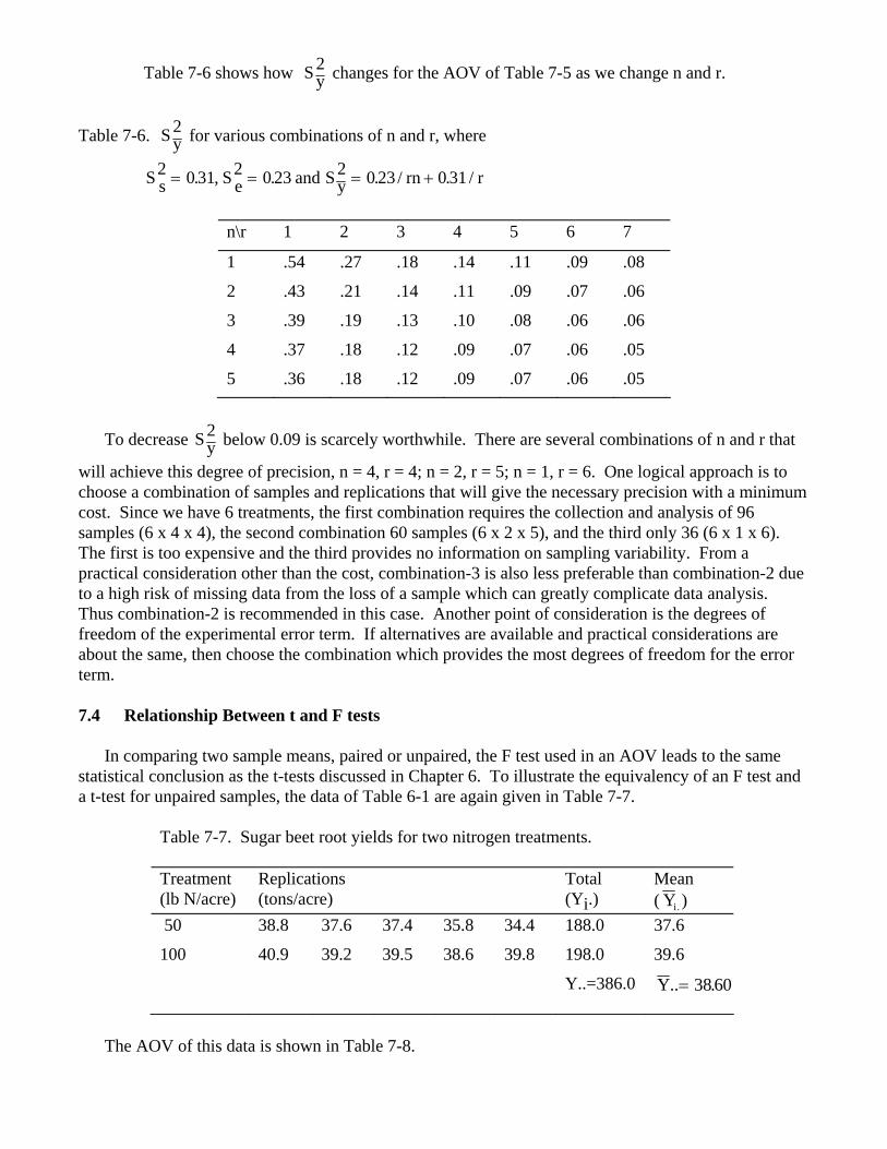
Table 7-6 shows how S y2 changes for the AOV of Table 7-5 as we change n and r.

Table 7-6. S y2 for various combinations of n and r, where

S s S e and S y rn r2 0 31 2 0 23 2 0 23 0 31= = = +. , . . / . /

n\r 1 2 3 4 5 6 7

1 .54 .27 .18 .14 .11 .09 .08

2 .43 .21 .14 .11 .09 .07 .06

3 .39 .19 .13 .10 .08 .06 .06

4 .37 .18 .12 .09 .07 .06 .05

5 .36 .18 .12 .09 .07 .06 .05

To decrease S y2 below 0.09 is scarcely worthwhile. There are several combinations of n and r that

will achieve this degree of precision, n = 4, r = 4; n = 2, r = 5; n = 1, r = 6. One logical approach is to choose a combination of samples and replications that will give the necessary precision with a minimum cost. Since we have 6 treatments, the first combination requires the collection and analysis of 96 samples (6 x 4 x 4), the second combination 60 samples (6 x 2 x 5), and the third only 36 (6 x 1 x 6). The first is too expensive and the third provides no information on sampling variability. From a practical consideration other than the cost, combination-3 is also less preferable than combination-2 due to a high risk of missing data from the loss of a sample which can greatly complicate data analysis. Thus combination-2 is recommended in this case. Another point of consideration is the degrees of freedom of the experimental error term. If alternatives are available and practical considerations are about the same, then choose the combination which provides the most degrees of freedom for the error term. 7.4 Relationship Between t and F tests In comparing two sample means, paired or unpaired, the F test used in an AOV leads to the same statistical conclusion as the t-tests discussed in Chapter 6. To illustrate the equivalency of an F test and a t-test for unpaired samples, the data of Table 6-1 are again given in Table 7-7.

Table 7-7. Sugar beet root yields for two nitrogen treatments. Treatment (lb N/acre)

Replications (tons/acre)

Total (Yi.)

Mean ( Yi. )

50 38.8 37.6 37.4 35.8 34.4 188.0 37.6

100 40.9 39.2 39.5 38.6 39.8 198.0 39.6

Y..=386.0 Y.. .= 38 60

The AOV of this data is shown in Table 7-8.

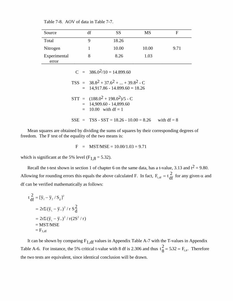
Table 7-8. AOV of data in Table 7-7. Source df SS MS F

Total 9 18.26

Nitrogen 1 10.00 10.00 9.71

Experimental 8 8.26 1.03 error

C = 386.02/10 = 14.899.60 TSS = 38.82 + 37.62 + ... + 39.82 - C = 14,917.86 - 14.899.60 = 18.26 STT = (188.02 + 198.02)/5 - C = 14,909.60 - 14,899.60 = 10.00 with df = 1 SSE = TSS - SST = 18.26 - 10.00 = 8.26 with df = 8 Mean squares are obtained by dividing the sums of squares by their corresponding degrees of freedom. The F test of the equality of the two means is: F = MST/MSE = 10.00/1.03 = 9.71 which is significant at the 5% level (F1,8 = 5.32). Recall the t-test shown in section 1 of chapter 6 on the same data, has a t-value, 3.13 and t2 = 9.80.

Allowing for rounding errors this equals the above calculated F. In fact, for any given α and

df can be verified mathematically as follows:

F t dfdf12

, =

t df y y S

r y y r Sdr y y r S r

d

i

i

2

2 2

2 2

1 22

2

2 2

= −

= −

= −

[ / ]

( ..) /

( ..) / ( /

.

.

Σ

Σ )

F .

= MST/MSE = F1,df It can be shown by comparing F1,df values in Appendix Table A-7 with the T-values in Appendix

Table A-6. For instance, the 5% critical t-value with 8 df is 2.306 and thus Therefore

the two tests are equivalent, since identical conclusion will be drawn.

t 28 532 1 8= =. ,

SUMMARY

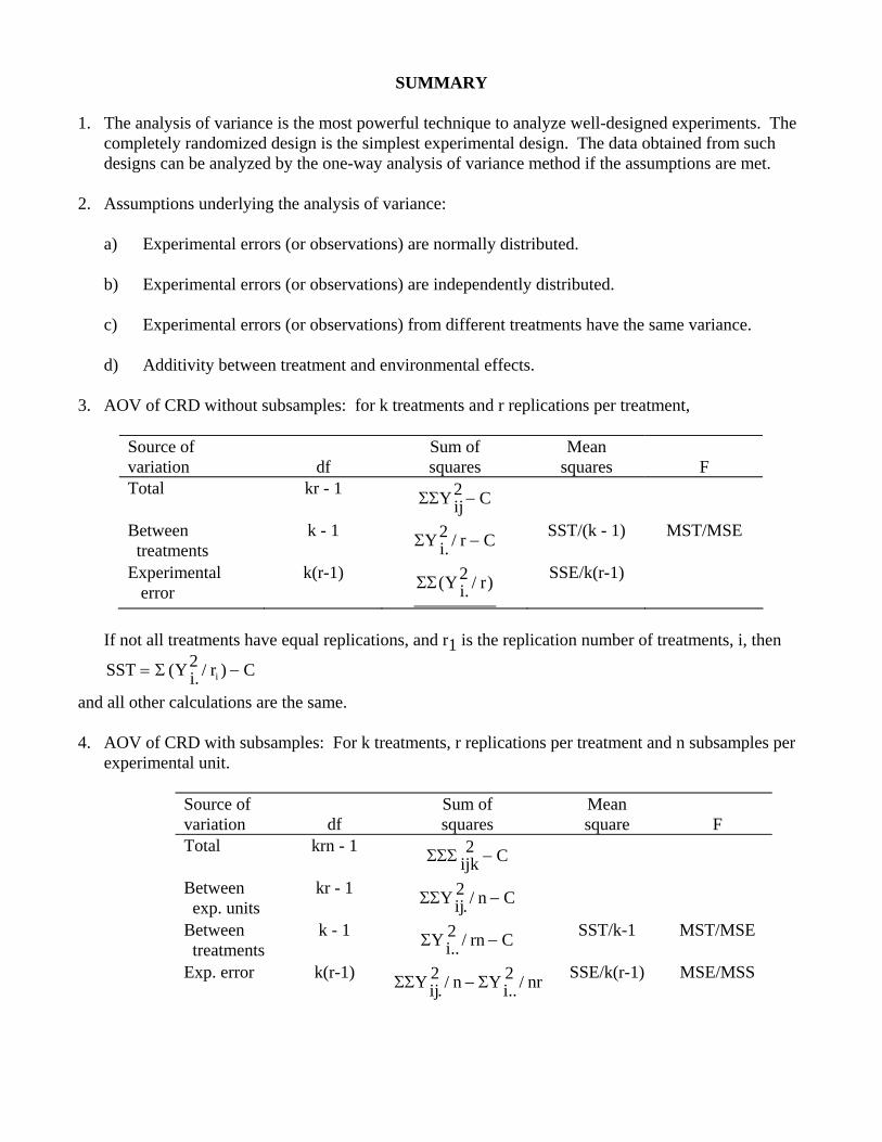
1. The analysis of variance is the most powerful technique to analyze well-designed experiments. The

completely randomized design is the simplest experimental design. The data obtained from such designs can be analyzed by the one-way analysis of variance method if the assumptions are met.

2. Assumptions underlying the analysis of variance: a) Experimental errors (or observations) are normally distributed. b) Experimental errors (or observations) are independently distributed. c) Experimental errors (or observations) from different treatments have the same variance. d) Additivity between treatment and environmental effects. 3. AOV of CRD without subsamples: for k treatments and r replications per treatment,

Source of variation

df

Sum of squares

Mean squares

F

Total kr - 1 ΣΣYij C2 −

Between treatments

k - 1 SST/(k - 1) MST/MSE ΣY i r C2. / −

Experimental k(r-1) ΣΣ( . / )Y i r2 error SSE/k(r-1)

If not all treatments have equal replications, and r1 is the replication number of treatments, i, then

SST Y i r Ci= −Σ ( . / )2

and all other calculations are the same. 4. AOV of CRD with subsamples: For k treatments, r replications per treatment and n subsamples per

experimental unit.

Source of variation

df

Sum of squares

Mean square

F

Total krn - 1 ΣΣΣ 2ijk C−

Between exp. units

kr - 1 ΣΣYij n C2. / −

Between treatments

k - 1 ΣYi rn C2.. / − SST/k-1 MST/MSE

Exp. error k(r-1) ΣΣ ΣYij n Yi nr2 2. / .. /−

SSE/k(r-1) MSE/MSS

SSS/kr(n-1) Sampling kr(n-1) ΣΣΣ ΣΣ2 2ijk ij n− . / error

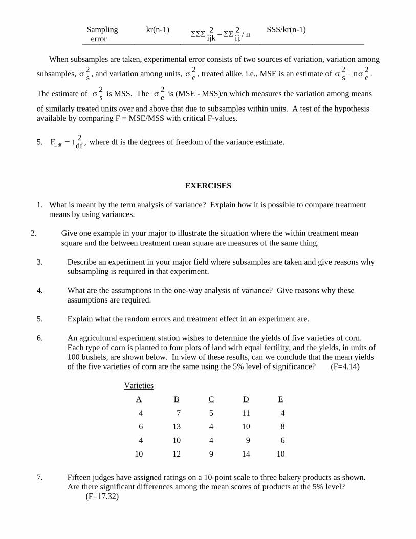
When subsamples are taken, experimental error consists of two sources of variation, variation among

subsamples, σ , and variation among units, σ , treated alike, i.e., MSE is an estimate of .

The estimate of is MSS. The σ is (MSE - MSS)/n which measures the variation among means

of similarly treated units over and above that due to subsamples within units. A test of the hypothesis available by comparing F = MSE/MSS with critical F-values.

2s

2e σ σ2 2

s n e+

σ2s

2e

5. where df is the degrees of freedom of the variance estimate. F t dfdf12

, ,=

EXERCISES 1. What is meant by the term analysis of variance? Explain how it is possible to compare treatment

means by using variances.

2. Give one example in your major to illustrate the situation where the within treatment mean square and the between treatment mean square are measures of the same thing.

3. Describe an experiment in your major field where subsamples are taken and give reasons why

subsampling is required in that experiment. 4. What are the assumptions in the one-way analysis of variance? Give reasons why these

assumptions are required. 5. Explain what the random errors and treatment effect in an experiment are. 6. An agricultural experiment station wishes to determine the yields of five varieties of corn.

Each type of corn is planted to four plots of land with equal fertility, and the yields, in units of 100 bushels, are shown below. In view of these results, can we conclude that the mean yields of the five varieties of corn are the same using the 5% level of significance? (F=4.14)

Varieties

A B C D E

4 7 5 11 4

6 13 4 10 8

4 10 4 9 6

10 12 9 14 10

7. Fifteen judges have assigned ratings on a 10-point scale to three bakery products as shown.

Are there significant differences among the mean scores of products at the 5% level? (F=17.32)

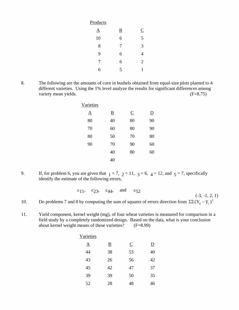
Products

A B C

10 6 5

8 7 3

9 6 4

7 6 2

6 5 1

8. The following are the amounts of corn in bushels obtained from equal-size plots planted to 4

different varieties. Using the 1% level analyze the results for significant differences among variety mean yields. (F=8.75)

Varieties

A B C D

80 40 80 90

70 60 80 90

80 50 70 80

90 70 90 60

40 80 60

40

9. If, for problem 6, you are given that 1 = 7, 2 = 11, 3 = 6, 4 = 12, and 5 = 7, specifically

identify the estimate of the following errors, ε11, ε23, ε44, and ε52

(-3, -1, 2, 1) 10. Do problems 7 and 8 by computing the sum of squares of errors direction from ΣΣ( ).Y yij i− 2 11. Yield component, kernel weight (mg), of four wheat varieties is measured for comparison in a

field study by a completely randomized design. Based on the data, what is your conclusion about kernel weight means of these varieties? (F=8.99)

Varieties

A B C D

44 38 53 40

43 26 56 42

45 42 47 37

39 39 50 35

52 28 48 46

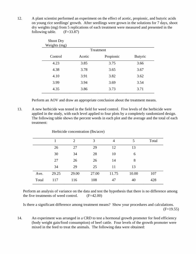
12. A plant scientist performed an experiment on the effect of acetic, propionic, and butyric acids

on young rice seedlings' growth. After seedlings were grown in the solutions for 7 days, shoot dry weights (mg) from 5 replications of each treatment were measured and presented in the following table. (F=33.87)

Shoot Dry

Weights (mg)

Treatment

Control Acetic Propionic Butyric

4.23 3.85 3.75 3.66

4.38 3.78 3.65 3.67

4.10 3.91 3.82 3.62

3.99 3.94 3.69 3.54

4.35 3.86 3.73 3.71

Perform an AOV and draw an appropriate conclusion about the treatment means.

13. A new herbicide was tested in the field for weed control. Five levels of the herbicide were

applied in the study, with each level applied to four plots by a completely randomized design. The following table shows the percent weeds in each plot and the average and the total of each treatment:

Herbicide concentration (lbs/acre)

1 2 3 4 5 Total

26 27 29 12 13

30 34 28 10 6

27 26 26 14 8

34 29 25 11 13

Ave. 29.25 29.00 27.00 11.75 10.00 107

Total 117 116 108 47 40 428

Perform an analysis of variance on the data and test the hypothesis that there is no difference among the five treatments of weed control. (F=42.00)

Is there a significant difference among treatment means? Show your procedures and calculations.

(F=19.55)

14. An experiment was arranged in a CRD to test a hormonal growth promoter for feed efficiency (body weight gain/food consumption) of beef cattle. Four levels of the growth promoter were mixed in the feed to treat the animals. The following data were obtained:

Treatment levels (100 ppm) Replication 1 2 3 4

1 0.065 0.070 0.082 0.095 2 0.061 0.081 0.089 0.091 3 0.058 0.086 0.090 0.097 4 0.072 0.074 0.093 0.110

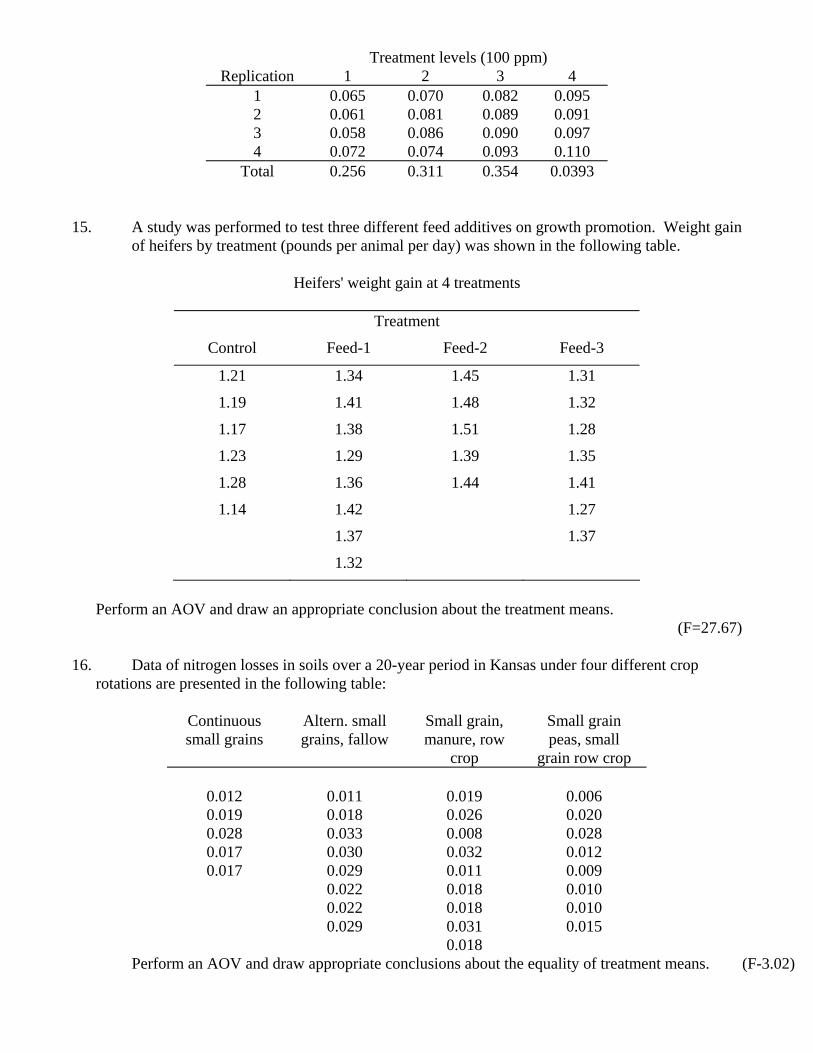
Total 0.256 0.311 0.354 0.0393 15. A study was performed to test three different feed additives on growth promotion. Weight gain

of heifers by treatment (pounds per animal per day) was shown in the following table.

Heifers' weight gain at 4 treatments

Treatment

Control Feed-1 Feed-2 Feed-3

1.21 1.34 1.45 1.31

1.19 1.41 1.48 1.32

1.17 1.38 1.51 1.28

1.23 1.29 1.39 1.35

1.28 1.36 1.44 1.41

1.14 1.42 1.27

1.37 1.37

1.32

Perform an AOV and draw an appropriate conclusion about the treatment means.

(F=27.67) 16. Data of nitrogen losses in soils over a 20-year period in Kansas under four different crop

rotations are presented in the following table:

Continuous small grains

Altern. small grains, fallow

Small grain, manure, row

crop

Small grain peas, small

grain row crop

0.012

0.011

0.019

0.006 0.019 0.018 0.026 0.020 0.028 0.033 0.008 0.028 0.017 0.030 0.032 0.012 0.017 0.029 0.011 0.009

0.022 0.018 0.010 0.022 0.018 0.010 0.029 0.031 0.015 0.018

Perform an AOV and draw appropriate conclusions about the equality of treatment means. (F-3.02)

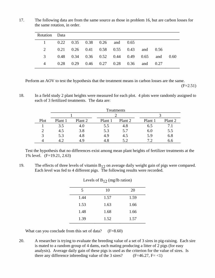
17. The following data are from the same source as those in problem 16, but are carbon losses for

the same rotation, in order.

Rotation Data

1 0.22 0.35 0.38 0.26 and 0.65

2 0.21 0.26 0.41 0.58 0.55 0.43 and 0.56

3 0.48 0.34 0.36 0.52 0.44 0.49 0.65 and 0.60

4 0.28 0.29 0.46 0.27 0.28 0.36 and 0.27

Perform an AOV to test the hypothesis that the treatment means in carbon losses are the same. (F=2.51)

18. In a field study 2 plant heights were measured for each plot. 4 plots were randomly assigned to

each of 3 fertilized treatments. The data are:

Treatments 1 2 3

Plot Plant 1 Plant 2 Plant 1 Plant 2 Plant 1 Plant 2 1 3.5 4.0 5.5 4.8 6.5 7.1 2 4.5 3.8 5.3 5.7 6.0 5.5 3 5.3 4.8 4.9 4.5 5.9 6.8 4 4.2 4.9 4.8 5.2 7.2 6.6

Test the hypothesis that no differences exist among mean plant heights of fertilizer treatments at the 1% level. (F=19.21, 2.63)

19. The effects of three levels of vitamin B12 on average daily weight gain of pigs were compared.

Each level was fed to 4 different pigs. The following results were recorded.

Levels of B12 (mg/lb ration)

5 10 20

1.44 1.57 1.59

1.53 1.63 1.66

1.48 1.68 1.66

1.39 1.52 1.57

What can you conclude from this set of data? (F=8.60)

20. A researcher is trying to evaluate the breeding value of a set of 3 sires in pig-raising. Each sire

is mated to a random group of 4 dams, each mating producing a litter of 2 pigs (for easy analysis). Average daily gain of these pigs is used as the criterion for the value of sires. Is there any difference inbreeding value of the 3 sires? (F=46.27, F= <1)

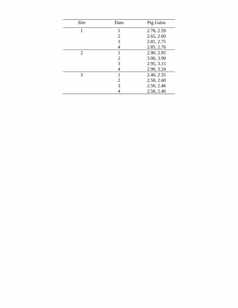
Sire Dam Pig Gains

1 1 2 3 4

2.78, 2.59 2.65, 2.60 2.81, 2.75 2.85, 2.76

2 1 2 3 4

2.90, 2.95 3.06, 3.90 2.95, 3.15 2.90, 3.24

3 1 2 3 4

2.46, 2.35 2.58, 2.60 2.50, 2.46 2.58, 2.40