STATSprofessor.com Chapter 7 Confidence Intervalsfaculty.fiu.edu/~mcguckd/LectureNotesSTATSICh7.pdf · We also present methods for determining sample sizes necessary to estimate those

STATSprofessor.com Chapter 7

1

Confidence Intervals

Recall: Inferential statistics are used to make predictions and decisions about a population based on

information from a sample. The two major applications of inferential statistics involve the use of sample

data to (1) estimate the value of a population parameter, and (2) test some claim (or hypothesis) about

a population.

In this Chapter, we introduce methods for estimating values of some important population parameters.

We also present methods for determining sample sizes necessary to estimate those parameters.

7.1 Finding Critical Z Values

The unknown population parameter that we are interested in estimating is called the target parameter.

Identifying the Target Parameter

Some helpful key words are provided below to determine our target parameter:

Parameter Key Words or Phrases Type of Data

Mean; Average Quantitative

p Proportion; Percentage; Fraction; Rate Qualitative

Estimating a Population Mean Using a Confidence Interval

Recall: A point estimator of a population parameter is a rule or formula that tells us how to use the sample data to calculate a single number that can be used to estimate the population parameter.

For all populations, the sample mean x is an unbiased estimator of the population mean , meaning that the distribution of sample means tends to center about the value of the

population mean . For many populations, the distribution of sample means x tends to be more consistent (with

less variation) than the distributions of other sample statistics.


2

We have used point estimators before to estimate target parameters; however, we cannot assign any

level of certainty with those point estimators. To remove this drawback, we can use what is called an

interval estimator.

An interval estimator (or Confidence Interval) is a formula that tells us how to use sample data to

calculate an interval that estimates a population parameter.

The confidence coefficient is the relative frequency with which the interval estimator encloses the

population parameter when the estimator is used repeatedly a very large number of times.

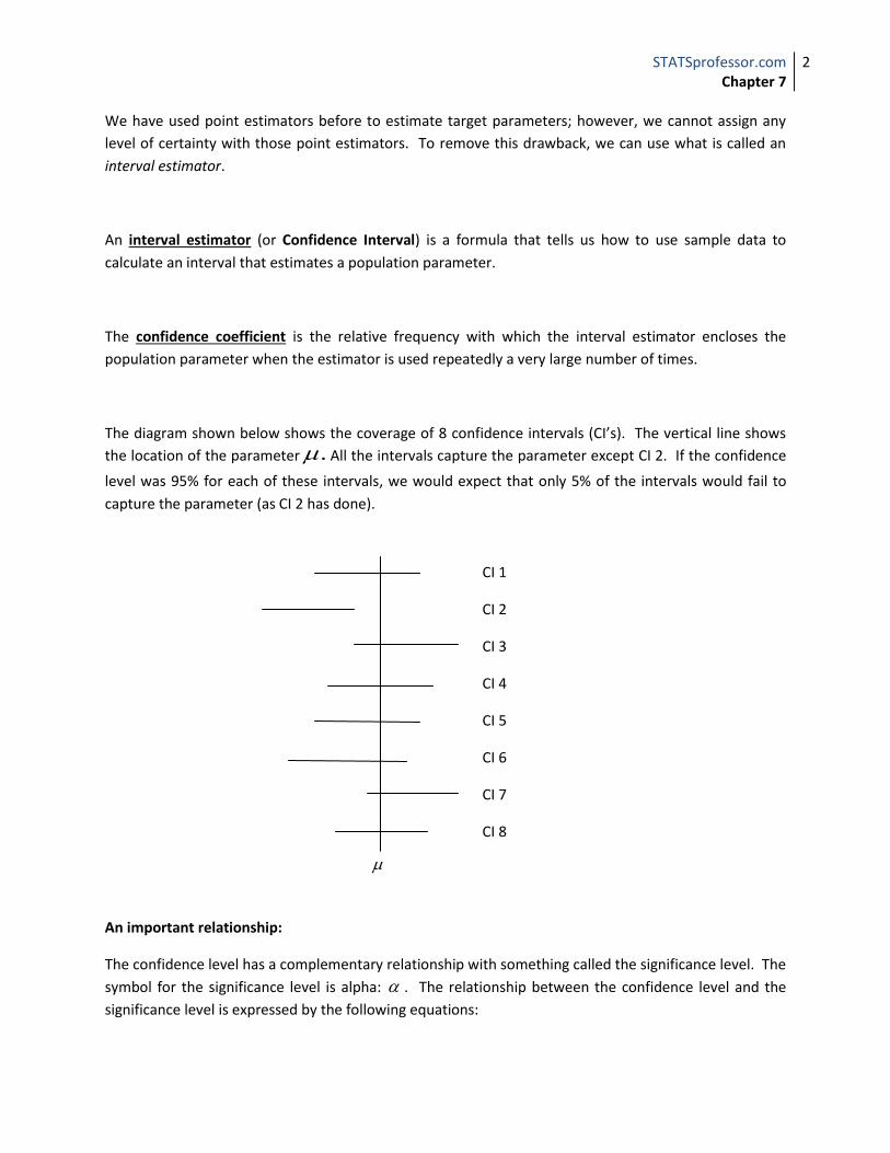
The diagram shown below shows the coverage of 8 confidence intervals (CI’s). The vertical line shows

the location of the parameter . All the intervals capture the parameter except CI 2. If the confidence

level was 95% for each of these intervals, we would expect that only 5% of the intervals would fail to

capture the parameter (as CI 2 has done).

An important relationship:

The confidence level has a complementary relationship with something called the significance level. The

symbol for the significance level is alpha: . The relationship between the confidence level and the

significance level is expressed by the following equations:

CI 1

CI 2

CI 3

CI 4

CI 5

CI 6

CI 7

CI 8


3

z

100% Significance Level Confidence Level

For example, if the confidence level is 90%, the significance level is 10%.

100% Confidence Level Significance Level

For example, if the significance level is 5%, the confidence level is 100% - 5% = 95%.

The most common choices for the confidence level are given below with the corresponding

significance levels: 90% (a = 10%), 95% (a = 5%), or 99% (a = 1%).

A little notation: The value z is defined as the value of the normal random variable Z such that the

area to its right is .

= area in this tail

Our goal for this section is to be able to estimate the true value of the population parameter (mu =

mean).

What we will need is sample data. This should include the sample mean, the sample size, and the

sample (or population) standard deviation. We will also need a confidence level and a z-chart.


4

Things Needed to Create a Confidence Interval for the Population Mean

Sample Mean x

Sample Size n

Standard Deviation

Confidence Level (1 - )100%

Z-table Value / 2z

The logic of a confidence interval can be understood by considering the following ideas. First, recall that

under the empirical rule approximately 95% of the data will fall between 2 standard deviations from

the mean. Also, recall that the CLT tells us that for samples of size n drawn from the population,

2~ , /x N n . (Note: 2~ , /x N n means the sample mean is normally distributed with

mean and variance 2 / n )

It should make sense that: 2 , 2x xn n

would capture about 95% of all the sample means

possible.

Now consider the drawing below:

The z score separating the right-tail is commonly denoted by z /2 and is referred to as a critical value

because it is on the borderline separating sample mean values that are likely to occur from those that

are unlikely to occur.


5

Sample means have a relatively small chance (with probability denoted by ) of falling in one of the

red tails of the figure.

Denoting the area of each shaded tail by /2, we see that there is a total probability of that a

sample mean will fall in either of the two red tails. By the rule of complements (from probability),

there is a probability of 1- that a sample mean will fall within the inner region of the figure below:

The critical value z/2 is the positive z value that is at the vertical boundary separating an area of /2 in

the right tail of the standard normal distribution. (The value of –z/2 is at the vertical boundary for the

area of /2 in the left tail.) The subscript /2 is simply a reminder that the z score separates an area

of /2 in the right tail of the standard normal distribution.

We can see from the drawing that the / 2 / 2 1P z Z z . Now, substitute for Z to get:

/ 2 / 2 1x

P z z

n

.

Next, we may solve the compound inequality for :

/ 2 / 2 1P z x zn n

,

1 – Alpha

/ 2z / 2z


6

Multiply all three sides of the inequality by negative one:

/ 2 / 2 1P z x zn n

,

Add x-bar to all three sides and write the inequality in the proper order:

/ 2 / 2 1P x z x zn n

,

Now, we must drop the probability notation because is not a random variable, but is instead an

unknown constant. The mean is either in the interval, or it isn’t.

Finally, we can say that we are (1 )100% that / 2 / 2x z x zn n

.

The (1 )100% Confidence Interval for the Mean

/ 2 / 2x z x zn n

*A note about notation: ,x E x E is often written as x E x E

The part of the interval above given by / 2z

n

is called the margin of error, E.


7

The margin of error is the maximum likely difference observed between the sample mean, x , and the

population mean, μ, and is denoted by E.

The formula above has only one quantity which we will not be given directly: / 2z

Here are the steps to finding / 2z (When a t-table can’t be used)

1. Identify the C-level 2. Find the (C-Level)/2 3. Go to the Z-table, (in the body of the table) look up the number found in step 2

4. / 2z = the bold numbers on the side and top of the table

Example 100: Find / 2z for a 95% confidence interval:

Solution: The confidence level is 0.95. Dividing that in two gives us: 0.4750. Looking up 0.4750 in our z-

table gives us our answer: / 2z = 1.96.

http://www.statsprofessor.com/video.php?chapterId=4&id=737#ptop


8

*** Note: Using the t-table provided with the formula card on my web site is much easier than the

above method. The t-table also provides an extra decimal place, so it is recommended to use the t-table

whenever possible.

Example 101: Find / 2z for a 90% CI

Example 102: Find / 2z for a 98% CI

Example 103: Find / 2z for a 99% CI.

Now that we can find / 2z , it will be easy to create our confidence intervals.

7.2 Large-Sample Confidence Intervals for a Population Mean

Before we create a confidence interval to estimate the mean, we should look at the requirements for

constructing these intervals:

1. The sample is a simple random sample. (All samples of the same size have an equal chance of being

selected.)

2. The value of the population standard deviation is known.

3. Either or both of these conditions are satisfied: The population is normally distributed or n > 30.

Steps to Create a Confidence Interval

1. List all given sample data from the problem including sample size and C-level

2. Find / 2z

3. Calculate the margin of error, / 2E zn

4. Calculate ,x E x E





9

Example 104: In sociology, a social network is defined as the people you make frequent contact with.

The personal network size for each adult in a sample of

2,819 adults was calculated. The sample had a mean

personal network size of 14.6 with a known population

standard deviation of 9.8.

a. Give a point estimate for the mean personal network size of all adults

b. Form a 95% confidence interval for the mean personal network size of all adults

c. Give the practical interpretation of the interval created in part b.

d. Give the conditions required for the interval to be valid (answer: The sample must be

random and n should be large, 30n ). !!!Important!!!

Example 105: A study found the body temperatures of 106 healthy adults.

The sample mean was 98.2 degrees and the sample standard deviation was

0.62 degrees. Find the margin of error E and the 95% confidence interval for

µ. Does the interval contradict the claim that the average body temperature

of healthy adults is 98.6 degrees?

Conclusion: There are some relationships that should be understood.

--If confidence goes up so does the interval width

-- If confidence goes down so does the interval width

--If sample size goes up interval width goes down

7.3 Determining the Sample Size




10

Sample Size for Estimating the Mean

Suppose we want to collect sample data with the objective of estimating some population. The

question is how many sample items must be obtained?

By solving the margin of error formula for n, we can arrive at the following sample size formula:

2

/ 2zn

E

where:

zα/2 = critical z score based on the desired confidence level

E = desired margin of error

σ = population standard deviation

When finding the sample size, n, if the use of the formula above does not result in a whole number,

always increase the value of n to the next larger whole number.

When solving a problem, you may see a phrase like, “We want to estimate the mean within ….” That

word within is a key word indicating the margin of error.

Example 106: Nielsen Media Research wants to estimate the mean time that full-time college students

spend watching TV each weekday. Find the sample size necessary to estimate that mean with a 15

minute margin of error. Assume that 96% confidence is desired, and assume that the population

standard deviation is 112.2 minutes.

http://www.statsprofessor.com/video.php?chapterId=4&id=741


11

Example 106.5: In a paper titled, “The Role of Deliberate Practice in the Acquisition of Expert

Performance” researchers estimated that it takes approximately 10,000 hours of deliberate practice to

become an expert at something. If we want to estimate the average time that it would take to become

an expert guitarist within 200 hours, how large should our sample of expert guitarists be? Assume the

standard deviation is 850 hours, and that we want a 95% confidence level.

7.4 Finding Critical T Values

Estimating a Population Mean: Small sample size (or σ unknown) and normally distributed.

This section presents methods for finding a confidence interval estimate of a population mean when the

population standard deviation is not known. With σ unknown, we will use the Student t distribution

assuming that certain requirements are satisfied.

Recall: The CLT says if 2~ ,X N , then 2~ , /X N n for any sample size n—no matter how

small.

However, if X is not normal we need a sufficiently large sample size to assume normality.

When the population standard deviation is unknown, we use the sample standard deviation (S) as a

substitute, but for small sample sizes S may not be a very good substitute.



12

Our goal for this section is to be able to estimate the true value of the population parameter (mu =

mean) when:

1. is unknown

2. The sample is normally distributed or 30n

*In class, we will use a simpler method for choosing between t and z. If 30n use z, otherwise use t.

In most cases, when the distribution is assumed to be normal, statisticians use the t-distribution, but

for in class problem solving (without software) the z distribution has some advantages. Thus in class,

we will use Z when our sample size is larger than 30.

As before, we will need certain information from the sample to form our confidence interval:

Things needed to create a Confidence Interval for the population mean

Sample Mean x

Sample Size n

Standard Deviation S

Confidence Level (1 - )100%

T-table Value / 2t

Note: we are no longer using a z value for our confidence interval; instead, we will need a value from a

related distribution: the Student’s t-distribution. The t-distribution has a shape like that of the standard

normal distribution (z-distribution), but it is a little heavier in the tails and, consequently, a little lower at

its center. The specific shape of the t-distribution is determined by its degrees of freedom = n – 1.

Important Properties of the Student t Distribution

1. The Student t distribution is different for different sample sizes (see the figures below).

2. The entire family of t distribution curves has a bell shape like the standard normal distribution,

but t distribution curves have standard deviations that are greater than one.


13

3. The Student t distribution has a mean of t = 0 (just as the standard normal distribution has a

mean of z = 0).

4. The standard deviation of the Student t distribution varies with the sample size and is greater

than 1 (unlike the standard normal distribution, which has a s = 1).

5. As the sample size n gets larger, the Student t distribution gets closer to the normal distribution.

* Z and t are related by taking a Standard Normal random variable (Z) and dividing it by the square root

of a Chi-squared random variable (V) which is divided by its degrees of freedom (v), we get a random

variable that has a Student’s t-distribution ( / /Z V v ).

0.025,4t


14

To get the needed critical value / 2t , we need to:

1. Get the degrees of freedom, df = n – 1

2. Find 1 CIlevel

3. Look-up the degrees of freedom and / 2 on the t-table from our site (or use any other t-table).

Example 107: Find / 2t for a 90% confidence interval with a sample size of n = 24

Example 108: Find / 2t for a 99% confidence interval with a sample size of n = 29

Example 109: Find 0t such that0( ) 0.025P t t when n = 28

Now that we can find / 2t , it is time to learn how to create our confidence interval to estimate the

mean:

7.5 Small-Sample Confidence Intervals for a Population Mean

Steps to Create a Confidence Interval

1. List all given sample data from the problem including sample size and C-level

2. Find / 2t

3. Calculate the margin of error, / 2

sE t

n

4. Calculate ,x E x E

Example 110: In a 2011 report by the CDF (Children’s Defense Fund), it was reported that a random

sample of 29 black males with only a high school degree earned on

average $25,418. The standard deviation is estimated to be $5,500. Use

the sample data and a 95% confidence level to find the margin of error E

and the confidence interval for µ. A 95% confidence interval was

constructed for white males, and it was found that the true mean income

for white males with only a high school degree was between $33,215 and

37,399. Comparing these two intervals, can we conclude there is a

significant difference between incomes for the two groups?






15

Example 111: Because cardiac deaths appear to increase after heavy snow falls, an experiment was

designed to determine the cardiac demands of manually shoveling snow. Ten subjects cleared tracts of

snow, and their maximum heart rates were recorded. Their average maximum heart rate was 175 with

a standard deviation of 15. Assuming maximum heart rates are normally distributed, find the 95%

confidence interval estimate of the population mean for those people who shovel snow manually.

Example 112: Flesch ease of reading scores for 12 different pages randomly selected from J.K. Rowling’s

Harry Potter and the Sorcerer’s Stone were calculated. Find

the 95% interval estimate of , the true mean Flesch ease of

reading score for Harry Potter and the Sorcerer’s Stone (The

12 pages’ distribution appears to be bell-shaped with x =

80.75 and s = 4.68).

Formal Method for Choosing Between z and t:

Method Conditions

Z-distribution known & normally distributed

or

known & n >30

t-distribution not known & normally distributed

or

not known & n >30

nonparametric Population is not normally distributed and

30n




16

*Note: for classroom purposes, we will use Z when 30n and t otherwise.

7.6 Confidence Intervals for a Population Proportion

Large-Sample Confidence Interval for a Population Proportion

In many real world scenarios, we would like to estimate a population proportion. If we look at n

randomly selected subjects and x of them have some trait we are interested in, we can form a sample

proportion from the data:

ˆx

pn

, where x = the number of subjects having the trait we are interested in.

This proportion is a sample proportion since it is only based on n subjects from some larger population.

We can use this ˆx

pn

to estimate the population proportion.


17

Since for each sample drawn of size n, a different amount (x) of subjects will have the desired trait, the

probabilities associated with each possible value of ˆx

pn

will be equal to the probability associated

with each possible value of x.

X has a binomial distribution—we can approximate this distribution when n is large (as long as n is large

enough that ˆˆ 3 pp will fit inside of 0,1 ) using the standard normal (Z) distribution.

Remember that X~binomial( np , 2 npq )

ˆx

pn

will have the following mean and standard deviation:

p̂ p and p̂

pq

n

To understand why these values are as they are look at the following properties of expectation:

E aX aE X and 2Var aX a Var X

Since E X np , X np

E pn n

Since Var X npq , 2

X npq pqVar

n n n

As before, we would like to have more than just a good point estimator of the population proportion, so

in this section, we will learn how to form an interval estimate of the true population proportion.

From above, we can recall the mean and standard deviation of ˆx

pn

is:

ˆx

E p E pn

, and p̂

pq

n


18

Now using the assumption that n is large, we can approximate the sampling distribution of ˆx

pn

by

the normal distribution.

Our interval to estimate the true population proportion will have a similar structure to the interval used

to estimate the mean:

(Point Estimate) (Number of Standard Deviations)(Standard Error)

/ 2

ˆ ˆˆ

pqp z

n

*Note: we are approximating the standard error of p̂ as,p̂

ˆ ˆpq

n

**Also, we should check that n is large enough that ˆˆ 3 pp will fit inside of 0,1 before using the

above method, or alternatively we can check to see if both 15n p and 15n q .

Steps to Creating a Confidence Interval for a Population Proportion:

1. Gather sample data: x (or p̂ ), n, and C-level [Calculate ˆx

pn

& (1 - p̂ ) = q̂ ]

2. Find / 2Z

3. Calculate the Margin of Error, E = / 2Z

ˆ ˆpq

n

4. Finally, form ˆ ˆ,p E p E

Example 113: A nationwide poll of nearly 1,500 people conducted by the syndicated cable television

show Dateline: USA found that 70 percent of those surveyed believe there is

intelligent life outside of Earth in the universe, perhaps even in our own Milky Way

Galaxy. What proportion of the entire population agrees, at the 95% confidence

level?



19

Example 113.5: In many sports, eligibility for minor leagues is determined by age at the start of the

calendar year (Jan 1). Journalist Malcolm Gladwell wrote about the effects of this eligibility rule on Canadian hockey in his 2008 book Outliers. The issue is that people born in the early months of the year end up being older when they are finally able to participate in minor leagues than students born in later months. For example, a child born on January 2nd who is eligible to play when he/she turns ten, will be 10 years and 364 days old when he starts playing compared to a child born December 31st who will only be 10 years

and 1 day old when he/she is eligible to play. Being older is an advantage in sports, so these older kids naturally perform better and stand out more to coaches and scouts.

Stephen Leavitt and Stephen J. Dubner, authors of the bestselling Freakonomics series of books, noted this trend in international soccer in a 2006 New York Times column. FIFA introduced a Jan. 1 cutoff date in 1997. Of the 410 players in the 2006 World Cup born after 1979 (thus affected by the Jan. 1 cutoff date) the percentage who were born in January, February and March was 32.4%. Use the 2006 World Cup Data and a 99% confidence level to form an interval estimate for the true proportion of FIFA players born after 1979 that have a birthday in the first three months of the year. Assuming that for the general population the

birth rate for the months January, February, and March is approximately 25%, does it seem the proportion of FIFA stars born in these three months is significantly higher than the expected 25% rate?

Example 114: Butt-dialing 911 is a growing problem. In New York City, a 2012 report stated that 40% of

calls made to 911 were dialed in error from cell phones. The

report looked at a sample of 743,000 calls handled by NYC’s 911

operators. Construct a 98% confidence interval estimate of the

true proportion of NYC 911 calls that are made in error. Before this

report the mayor of NYC claimed that more than 45% of the calls

made to 911 were due to “butt-dialing.” Did this report contradict

the mayor’s claim?

Example 115: When Mendel conducted his famous genetics experiments with peas,

one sample of offspring consisted of 428 green peas and 152 yellow peas. Mendel

expected that 25% of the offspring peas would be yellow. Find a 95% confidence

interval estimate for the true proportion of yellow peas. Do the results contradict

Mendel’s theory?

Messi, in his Barca uniform above, born in late June probably did not benefit from his date of birth, but the cry baby in the white Real Madrid

uniform was born in early Feb and probably did benefit from his lucky birth month… just another reason why Messi is the better player.





20

Note: Watch out for problems where p is very close to 0 or 1, in those cases, n would have to be very

large for the sampling distribution of p̂ to be well approximated by the normal curve.

If p is close to 0 or 1, Wilson’s adjustment for estimating p yields better results

/ 2

(1 )

4

2

4

p pp z

n

xp

n

where

Example 116: Suppose in a particular year the percentage of firms declaring bankruptcy that had shown

profits the previous year is .002. If 100 firms are sampled and one had declared bankruptcy, what is the

95% CI on the proportion of profitable firms that will tank the next year?

Solution:

/ 2

(1 )

4

2 1 2.0289

4 100 4

.0289(1 .0289).0289 1.96

100 4

.0289 .032

p pp p z

n

xp

n

p

p

Determining Sample Size for the Estimation of Proportion

If we want to estimate the population proportion with a certain margin of error and a specified

confidence level, we will use the following formula to determine the needed sample size:

2

/2

2

z pqn

E

Where p and q can be estimated from previously known sample data or can be conservatively estimated

to be 0.50 each. The formula above was derived by solving the formula for margin of error for n.

Documents

STATSprofessor.com Chapter 7 Confidence Intervalsfaculty.fiu.edu/~mcguckd/LectureNotesSTATSICh7.pdf · We also present methods for determining sample sizes necessary to estimate those