CHAPTER 7 Convergence Acceleration

7
CHAPTER 7 Convergence Acceleration
In CFL3D, the convergence rate at which many problems are solved can be accelerated with the use of multigrid, mesh sequencing, or a combination of the two. The following sections describe the two techniques. The use of multigrid with grid overlapping and embedded grids is also discussed.

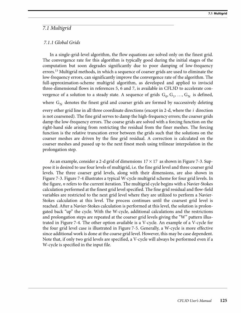
Multigrid is a highly recommended option available in CFL3D. The improvement in convergence acceleration afforded with multigrid makes it very worthwhile to learn about and utilize. Table 7–1 illustrates this fact for two cases, a 2-d airfoil and a 3-d forebody. A work unit is defined here to be the “equivalent” fine grid iteration. For example, on the fin-est grid level, 1 iteration = 1 work unit; on the next-to-finest grid level, 1 iteration = 1/8 (1/4 in 2-d) of a work unit; on the next coarser level, 1 iteration = 1/64 (1/16 in 2-d) of a work unit; and so forth. The residual and lift coefficient convergence histories for these two cases are shown in Figure 7-1 and Figure 7-2. The term “full multigrid” implies that mesh sequencing is used in conjunction with multigrid. See “Mesh Sequencing” on page 134. Note that there is an additional CPU penalty for the overhead associated with the multigrid scheme that is not reflected in the work unit measure, however, for most problems, the overhead is small.

Table 7–1. Convergence improvements with multigrid.

Case

Approximate Number of Work Units to Achieve the Final Lift

Without Multigrid With Multigrid With Full-Multigrid

2-d NACA 4412 Airfoil 10,000 1000 750

3-d F-18 Forebody >> 1500* 500 500

*This case was stopped after 1500 iterations when it became clear that the lift coefficient was far from converged and

to continue running the case would have been a waste of computer resources.

CFL3D User’s Manual 123


124

Figure 7-1. Convergence acceleration for 2-d NACA 4412 airfoil case.

0 500 1000-10

-9

-8

-7

-6

-5

-4

-3

Work

Log(R)

Full MG

MG

No MG

0 500 10000.300

0.350

0.400

0.450

0.500

Work

CL

Note: result without multigrid

requires O(10,000) work units

not shown for clarity

to converge to same CL value;

Full MG

MG

α = 0.0° M∞ = 0.2 Rec = 1.5×106 Spalart-Allmaras ModelMultigrid Acceleration - NACA 4412 Airfoil

Figure 7-2. Convergence acceleration for 3-d F-18 Forebody case.

0 500 1000 1500-6

-5

-4

-3

-2

-1

0

1

Work

Log(R)

Full Multigrid

Multigrid

Without Multigrid

0 500 1000 15000.100

0.150

0.200

0.250

0.300

0.350

0.400

Work

CL

Full Multigrid

Multigrid

Without Multigrid

Multigrid Acceleration - F/A-18 Forebodyα = 30.0° M∞ = 0.34 Rec = 13.5×106 Spalart-Allmaras Model 5 Patched Zones

CFL3D User’s Manual

7.1 Multigrid

7.1 Multigrid

7.1.1 Global Grids

In a single-grid-level algorithm, the flow equations are solved only on the finest grid. The convergence rate for this algorithm is typically good during the initial stages of the computation but soon degrades significantly due to poor damping of low-frequency

errors.13 Multigrid methods, in which a sequence of coarser grids are used to eliminate the low-frequency errors, can significantly improve the convergence rate of the algorithm. The full-approximation-scheme multigrid algorithm, as developed and applied to inviscid three-dimensional flows in references 5, 6 and 7, is available in CFL3D to accelerate con-

vergence of a solution to a steady state. A sequence of grids G0 G1 … GN, , , is defined,

where GN denotes the finest grid and coarser grids are formed by successively deleting

every other grid line in all three coordinate directions (except in 2-d, where the i direction

is not coarsened). The fine grid serves to damp the high-frequency errors; the coarser grids damp the low-frequency errors. The coarse grids are solved with a forcing function on the right-hand side arising from restricting the residual from the finer meshes. The forcing function is the relative truncation error between the grids such that the solutions on the coarser meshes are driven by the fine grid residual. A correction is calculated on the coarser meshes and passed up to the next finest mesh using trilinear interpolation in the prolongation step.

As an example, consider a 2-d grid of dimensions 17 17× as shown in Figure 7-3. Sup-

pose it is desired to use four levels of multigrid, i.e. the fine grid level and three coarser grid levels. The three coarser grid levels, along with their dimensions, are also shown in Figure 7-3. Figure 7-4 illustrates a typical W-cycle multigrid scheme for four grid levels. In the figure, n refers to the current iteration. The multigrid cycle begins with a Navier-Stokes calculation performed at the finest grid level specified. The fine grid residual and flow-field variables are restricted to the next grid level where they are utilized to perform a Navier-Stokes calculation at this level. The process continues until the coarsest grid level is reached. After a Navier-Stokes calculation is performed at this level, the solution is prolon-gated back “up” the cycle. With the W-cycle, additional calculations and the restrictions and prolongation steps are repeated at the coarser grid levels giving the “W” pattern illus-trated in Figure 7-4. The other option available is a V-cycle. An example of a V-cycle for the four grid level case is illustrated in Figure 7-5. Generally, a W-cycle is more effective since additional work is done at the coarse grid level. However, this may be case dependent. Note that, if only two grid levels are specified, a V-cycle will always be performed even if a W-cycle is specified in the input file.



126

Figure 7-3. Fine grid and coarse grid levels.

GN: 17 × 17 GN–1: 9 × 9

GN–2: 5 × 5 GN–3: 3 × 3

Figure 7-4. Multigrid W-cycle.

Grid

N

N-1

N-2

N-3

NS

NS

NS

NSNS

NS

NS

NS

NS

NS

NS

NS

R

RP P

P

R

R R R RP P P P

NS: Navier-Stokes CalculationR: Residual/q RestrictionP: Prolongation

qn+1qn


7.1.2 A Word About Grid Dimensions

Figure 7-5. Multigrid V-cycle.

NS

NS

NS

NS

NSR

RP

P

RP

NS: Navier-Stokes CalculationR: Residual/q RestrictionP: Prolongation Grid

N

N-1

N-2

N-3

qn+1qn

For a multigrid W-cycle, the pertinent lines of input for the example in Figure 7-3 would look something like:

Line Type5 DT IREST IFLAGTS FMAX IUNST CFLTAU

-1.0 0 0 1.0 0 10.06 NGRID NPLOT3D NPRINT NWREST ICHK I2D NTSTEP ITA

1 0 0 0 0 1 1 17 NCG IEM IADVANCE IFORCE IVISC(I) IVISC(J) IVISC(K)

3 0 0 1 0 0 08 IDIM JDIM KDIM

2 17 1720 MSEQ MGFLAG ICONSF MTT NGAM

1 1 0 0 222 NCYC MGLEVG NEMGL NITFO

200 4 0 023 MIT1 MIT2 MIT3 MIT4 MIT5

1 1 1 1 1


When determining how many multigrid levels are available for a particular grid, use the following formula:

mcm f 1–

2--------------- 1+

m f 1+

2---------------= = (7-1)

where m f is a fine-grid dimension (idim, jdim, or kdim) and mc is the corresponding

coarse-grid dimension. Then rename mc as m f and compute Equation (7-1) again to

determine an even coarser grid dimension. When mc is an even number, that is as coarse

as that grid dimension can go.



128

For example, suppose a grid has idim = 37, jdim = 65, kdim = 65. The coarse grid below that would have idim = 19, jdim = 33, kdim = 33. The next coarser grid would have idim = 10, jdim = 17, kdim = 17. Since idim is an even number, that is as coarse as the grid can go; even though jdim and kdim can be reduced to coarser numbers, the entire grid is restricted by the idim = 10 value.

If the use of multigrid is desirable, it is important to plan ahead in the grid generation step of the computational problem. Choose grid dimensions that are “good” multigrid numbers, such as 129 (65, 33, 17, 9, 5, 3), 73 (37, 19), and 49 (25, 13, 7). Generally, two or three coarser grid levels are satisfactory.

It is best if all grid segments are also multigridable (see “LT14 - I0 Boundary Condition Specification” on page 32 through “LT19 - KDIM Boundary Condition Specification” on

page 35). For example, a face with jdim = 65 might have a portion from j = 1 to 17 as a

one-to-one interface, a portion from j = 17 to 41 as a viscous wall, and a portion from j =

41 to 65 as a patched interface. Each of these segment lengths (7, 25, and 25) is multigrid-able down three levels. Note that CFL3D will sometimes work fine even if some grid seg-ments are not multigridable: the code can assign indices on the coarser levels that denote different physical locations than the indices on the fine grid and still converge on the finest level. However, this does not work all the time. For example, if a C-mesh has a wrap-

around dimension of jdim = 257 and the wake extends from j = 1 to 40 and j = 218 to 257

(with one-to-one point matching), the code will create a coarser level with the wake from j

= 1 to 20 and j = 109 to 129 (using Equation (7-1)). On this level, j = 20 is a physically dif-ferent point from j = 109 (it is not even the actual trailing edge), and will yield a boundary condition error when the code is run, because these points are expected to match in a one-to-one fashion. It is currently not necessary to specify laminar regions with multigridable numbers. See Note (3) on page 29 in the LT9 - Laminar Region Specification description.

It is also important to consider the grid geometry when defining the grid dimensions. If multigrid is used, be sure to have any important geometric features (such as corners) located at multigridable points. Otherwise, on coarser levels, the geometry may change sig-nificantly, resulting in poor multigrid performance.



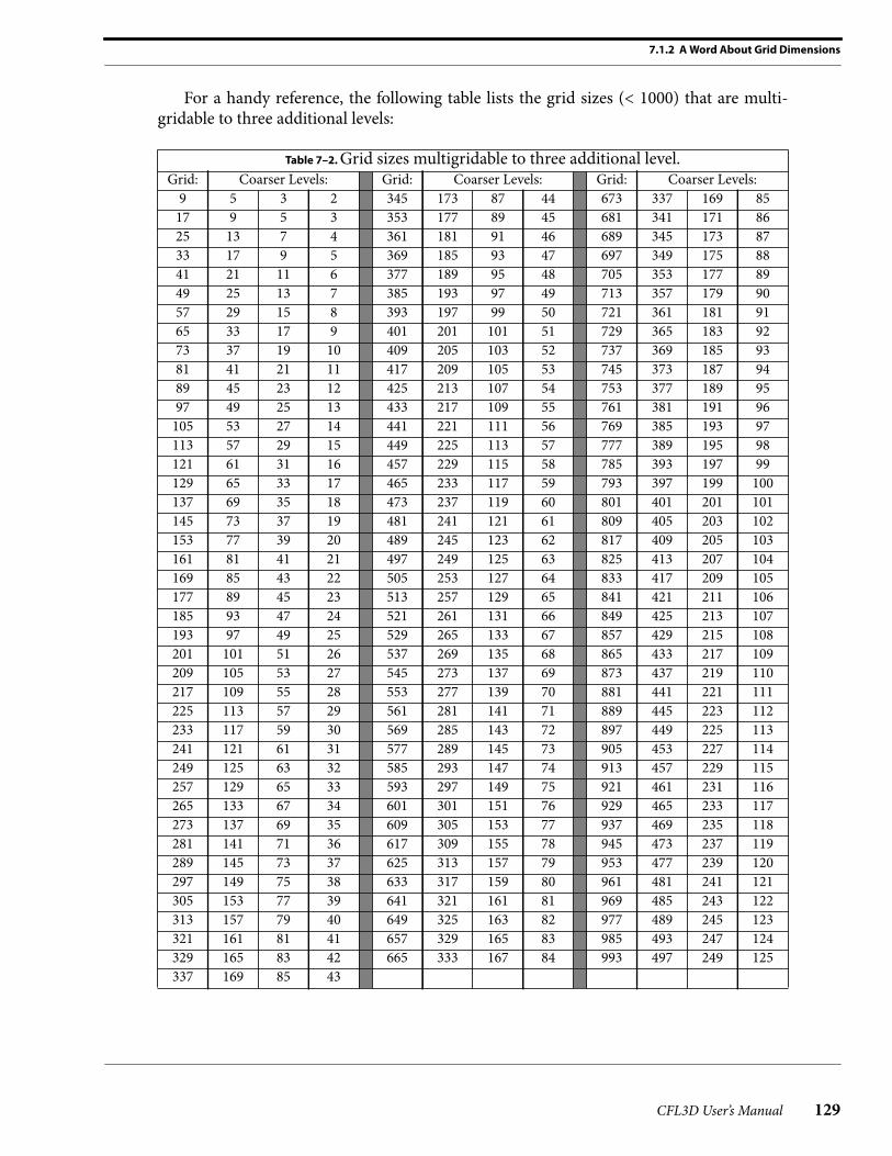
For a handy reference, the following table lists the grid sizes (< 1000) that are multi-gridable to three additional levels:

Table 7–2. Grid sizes multigridable to three additional level.Grid: Coarser Levels: Grid: Coarser Levels: Grid: Coarser Levels:

9 5 3 2 345 173 87 44 673 337 169 85

17 9 5 3 353 177 89 45 681 341 171 86

25 13 7 4 361 181 91 46 689 345 173 87

33 17 9 5 369 185 93 47 697 349 175 88

41 21 11 6 377 189 95 48 705 353 177 89

49 25 13 7 385 193 97 49 713 357 179 90

57 29 15 8 393 197 99 50 721 361 181 91

65 33 17 9 401 201 101 51 729 365 183 92

73 37 19 10 409 205 103 52 737 369 185 93

81 41 21 11 417 209 105 53 745 373 187 94

89 45 23 12 425 213 107 54 753 377 189 95

97 49 25 13 433 217 109 55 761 381 191 96

105 53 27 14 441 221 111 56 769 385 193 97

113 57 29 15 449 225 113 57 777 389 195 98

121 61 31 16 457 229 115 58 785 393 197 99

129 65 33 17 465 233 117 59 793 397 199 100

137 69 35 18 473 237 119 60 801 401 201 101

145 73 37 19 481 241 121 61 809 405 203 102

153 77 39 20 489 245 123 62 817 409 205 103

161 81 41 21 497 249 125 63 825 413 207 104

169 85 43 22 505 253 127 64 833 417 209 105

177 89 45 23 513 257 129 65 841 421 211 106

185 93 47 24 521 261 131 66 849 425 213 107

193 97 49 25 529 265 133 67 857 429 215 108

201 101 51 26 537 269 135 68 865 433 217 109

209 105 53 27 545 273 137 69 873 437 219 110

217 109 55 28 553 277 139 70 881 441 221 111

225 113 57 29 561 281 141 71 889 445 223 112

233 117 59 30 569 285 143 72 897 449 225 113

241 121 61 31 577 289 145 73 905 453 227 114

249 125 63 32 585 293 147 74 913 457 229 115

257 129 65 33 593 297 149 75 921 461 231 116

265 133 67 34 601 301 151 76 929 465 233 117

273 137 69 35 609 305 153 77 937 469 235 118

281 141 71 36 617 309 155 78 945 473 237 119

289 145 73 37 625 313 157 79 953 477 239 120

297 149 75 38 633 317 159 80 961 481 241 121

305 153 77 39 641 321 161 81 969 485 243 122

313 157 79 40 649 325 163 82 977 489 245 123

321 161 81 41 657 329 165 83 985 493 247 124

329 165 83 42 665 333 167 84 993 497 249 125

337 169 85 43



130

7.1.3 Overlapped Grids

With the grid-overlapping scheme, interpolation stencils are determined at the finest grid level only. Therefore, information would be missing at the coarser grid levels of the multigrid scheme. To avoid the need to obtain interpolation stencils at the coarser grid lev-els prior to the computation and the corresponding problems that most likely will arise, the

multigrid scheme has been modified to accommodate grid-overlapping cases.24

First, if a fine grid boundary is supplied overlap information as the boundary condi-tion, extrapolation is used for that boundary condition on all coarser grids. Second, for the restriction step of the multigrid scheme, all points are interpolated to coarser grids regard-less of whether or not they are in a hole at the fine grid level. The flow variables in the hole are simply at free-stream conditions. Finally, for the prolongation step, only corrections on field points are used to update the finest mesh solution. The hole points are not updated since they will be overwritten with free-stream values when a Navier-Stokes calculation is made at each fine grid level. Likewise, the fringe points are not corrected since they will be updated with flow information from other grids at the same fine grid level.

Note that in Chapter 3 under “LT20 - Mesh Sequencing and Multigrid” on page 35, it is stated that the W-cycle is not recommended with overlapped grids. Therefore, set ngam = 1.

7.1.4 Embedded Grids

For time advancement, embedded grids basically become an extension of the multigrid scheme. Consider the grid system shown in Figure 7-6. The finest global grid has dimen-

sions 9 9× and there are two coarser global grids for multigrid purposes. In addition,

there is a 7 13× grid embedded in the finest global grid as shown in the figure. The multi-

grid (W-cycle) scheme would follow the course drawn in Figure 7-7.



Figure 7-6. One embedded mesh in finest global grid.

GN: 9 × 9

GN–1: 5 × 5 GN–2: 3 × 3

GN+1: 7 × 13

Figure 7-7. Multigrid W-cycle with one embedded grid level.

NS

NS

NS

NSNS

NS

NS

R

RP

R RP P

NS: Navier-Stokes CalculationR: Residual/q RestrictionP: Prolongation Grid

N+1

N

N-1

N-2

qn+1qn

P



132

For a multigrid W-cycle, the pertinent lines of input for the example in Figure 7-6would look something like:




2 0 0 1 0 0 00 1 0 0 0 0 0

8 IDIM JDIM KDIM2 9 92 7 13

10 INEWG IGRIDC IS JS KS IE JE KE0 0 0 0 0 0 0 00 1 1 4 1 2 7 7

20 MSEQ MGFLAG ICONSF MTT NGAM1 1 1 0 2

22 NCYC MGLEVG NEMGL NITFO200 3 1 0

23 MIT1 MIT2 MIT3 MIT4 MIT51 1 1 1 1

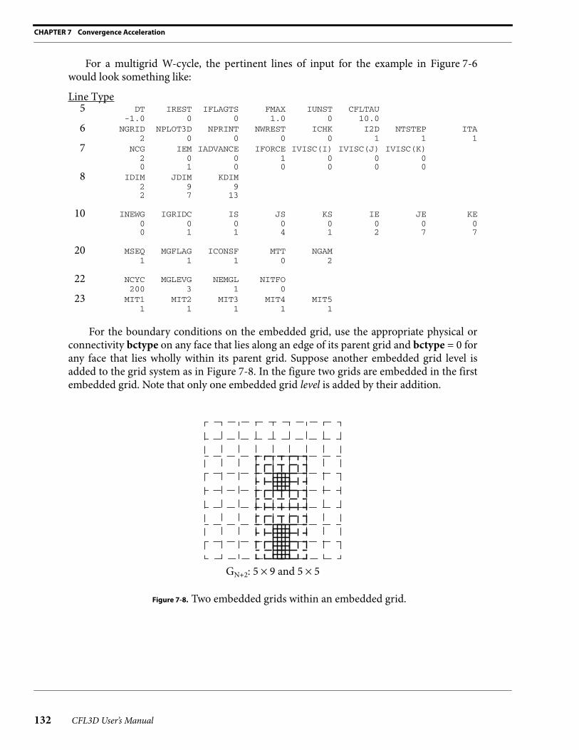
For the boundary conditions on the embedded grid, use the appropriate physical or connectivity bctype on any face that lies along an edge of its parent grid and bctype = 0 for any face that lies wholly within its parent grid. Suppose another embedded grid level is added to the grid system as in Figure 7-8. In the figure two grids are embedded in the first embedded grid. Note that only one embedded grid level is added by their addition.

Figure 7-8. Two embedded grids within an embedded grid.

GN+2: 5 × 9 and 5 × 5



The corresponding input would resemble:




2 0 0 1 0 0 00 1 0 0 0 0 00 2 0 0 0 0 00 2 0 0 0 0 0

8 IDIM JDIM KDIM2 9 92 7 132 5 92 5 5

10 INEWG IGRIDC IS JS KS IE JE KE0 0 0 0 0 0 0 00 1 1 4 1 2 7 71 2 1 3 1 2 5 51 2 1 3 9 2 5 11




Note that inewg should be set to 0 for grids 3 and 4 if this case is restarted.

Multigrid can also be performed at the embedded grid levels themselves by setting mgflag = 2. The embedded grid uses the coarser grid levels in which it is embedded, so ncg for the embedded grid itself should remain 0. The input for this case would resemble:




2 0 0 1 0 0 00 1 0 0 0 0 0

8 IDIM JDIM KDIM2 9 92 7 13

10 INEWG IGRIDC IS JS KS IE JE KE0 0 0 0 0 0 0 00 1 1 4 1 2 7 7






134

7.2 Mesh Sequencing

When setting up a CFD problem, initial conditions are set at every point on a grid. Usually, the closer the guess is to the final solution the quicker the case will converge. In CFL3D, the initial conditions for a problem are set at free-stream conditions for a single-grid-level case. However, if mesh sequencing is utilized, a better “guess” can be made for the initial conditions on the finer grid where the computations are most expensive.

Suppose a solution is desired on the 9 9× grid depicted in Figure 7-9. Instead of start-

ing the solution with free-stream conditions, a solution could first be obtained on the

5 5× grid shown in Figure 7-10. While the solution on the 9 9× grid would be more

accurate than that on the 5 5× grid, the coarser grid’s solution would be closer to the fine

grid solution than free-stream conditions. Since the coarse grid solution can be computed more quickly than the fine grid solution, it is usually beneficial to use the coarse grid solu-tion as the initial condition for the fine grid.

Figure 7-9. Simple grid example.

9 × 9

Figure 7-10. Mesh sequencing sample grid.

5 × 5

There are two ways to implement mesh sequencing in CFL3D. The first way is to com-pletely converge the solution on the coarse grid before mapping it up to the fine grid. For the sample grids, the pertinent input would look like:




7.2 Mesh Sequencing



2 9 9




1 1 1 1 11 1 1 1 1

Note that multigrid is also employed. The coarse grid solution can be examined and, if the solution on the coarse grid is not converged, the case can be restarted on that grid. After the coarse grid solution is converged, the solution is mapped to the fine grid and the calculations continue at the fine grid level. The pertinent input for this step would look something like:





2 9 9




1 1 1 1 11 1 1 1 1

Here, one iteration is performed on the coarse grid and two-hundred iterations are per-formed on the fine grid. At the end of this run, only the fine grid solution is available for examination. (So be sure to save the coarse grid solution before this step if it will be needed later for grid refinement studies, etc.) The case can be resubmitted for additional computa-tions on the fine grid with the following input:





2 9 9

20 MSEQ MGFLAG ICONSF MTT NGAM



136

1 1 0 0 1



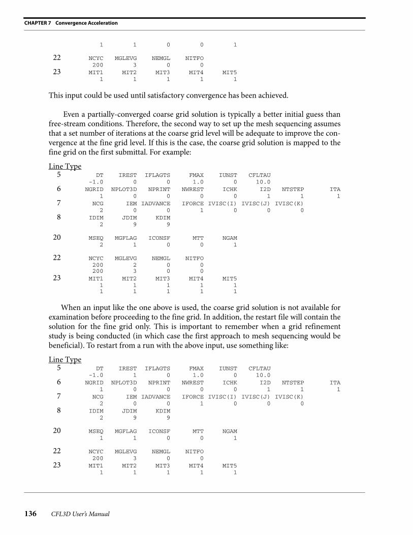
This input could be used until satisfactory convergence has been achieved.

Even a partially-converged coarse grid solution is typically a better initial guess than free-stream conditions. Therefore, the second way to set up the mesh sequencing assumes that a set number of iterations at the coarse grid level will be adequate to improve the con-vergence at the fine grid level. If this is the case, the coarse grid solution is mapped to the fine grid on the first submittal. For example:





2 9 9


22 NCYC MGLEVG NEMGL NITFO200 2 0 0200 3 0 0

23 MIT1 MIT2 MIT3 MIT4 MIT51 1 1 1 11 1 1 1 1

When an input like the one above is used, the coarse grid solution is not available for examination before proceeding to the fine grid. In addition, the restart file will contain the solution for the fine grid only. This is important to remember when a grid refinement study is being conducted (in which case the first approach to mesh sequencing would be beneficial). To restart from a run with the above input, use something like:





2 9 9





7.2 Mesh Sequencing

One last note about mesh sequencing is to emphasize, as with multigrid, the advantage of “good” grid dimensions. See “A Word About Grid Dimensions” on page 127. Planning for mesh sequencing should be made at the grid generation step of the CFD problem.



138

Documents

CHAPTER 7 Convergence Acceleration