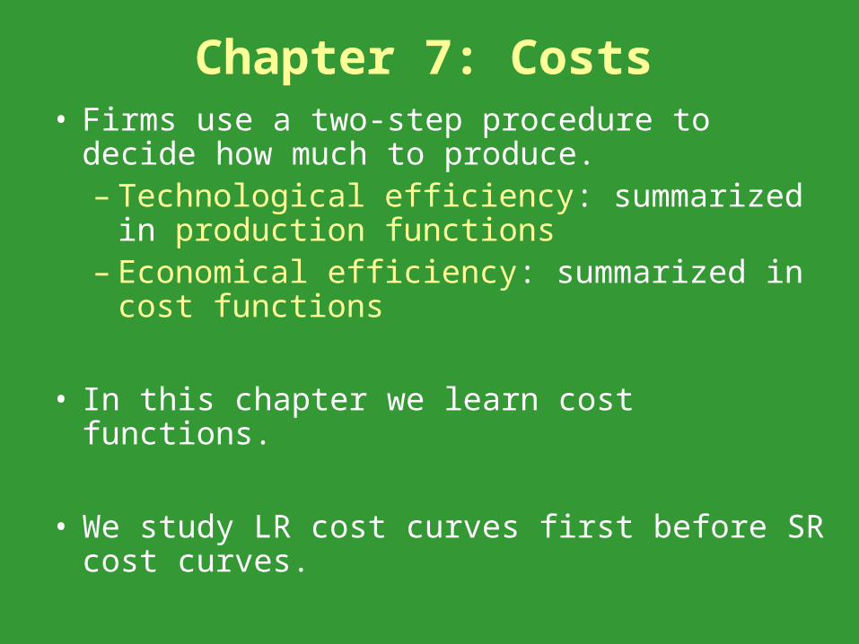
Chapter 7: Costs• Firms use a two-step procedure to decide how

much to produce.– Technological efficiency: summarized in

production functions– Economical efficiency: summarized in cost

functions

• In this chapter we learn cost functions.

• We study LR cost curves first before SR cost curves.

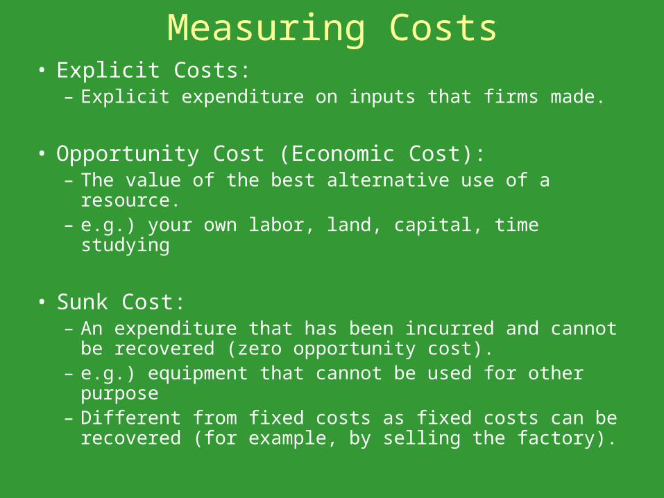
Measuring Costs• Explicit Costs:

– Explicit expenditure on inputs that firms made.

• Opportunity Cost (Economic Cost):– The value of the best alternative use of a resource.– e.g.) your own labor, land, capital, time studying

• Sunk Cost:– An expenditure that has been incurred and cannot be

recovered (zero opportunity cost).– e.g.) equipment that cannot be used for other purpose– Different from fixed costs as fixed costs can be

recovered (for example, by selling the factory).

Deriving Cost Curves

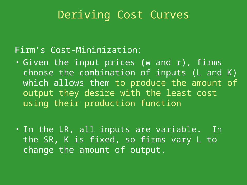
Firm’s Cost-Minimization:• Given the input prices (w and r), firms choose the

combination of inputs (L and K) which allows them to produce the amount of output they desire with the least cost using their production function

• In the LR, all inputs are variable. In the SR, K is fixed, so firms vary L to change the amount of output.

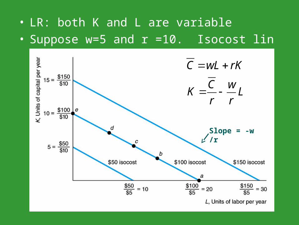
• LR: both K and L are variable• Suppose w=5 and r =10. Isocost lines are:

C wL rK

C wK L

r r

Slope = -w/r

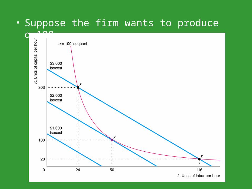
• Suppose the firm wants to produce q=100.

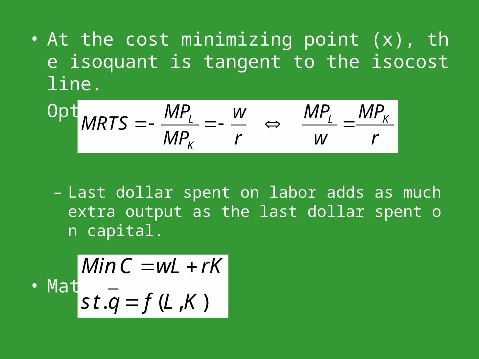
• At the cost minimizing point (x), the isoquant is tangent to the isocost line.

Optimum condition:

– Last dollar spent on labor adds as much extra output as the last dollar spent on capital.

• Mathematically,

L L K

K

MP MP MPwMRTS

MP r w r

. . ( , )

Min C wL rK

s t q f L K

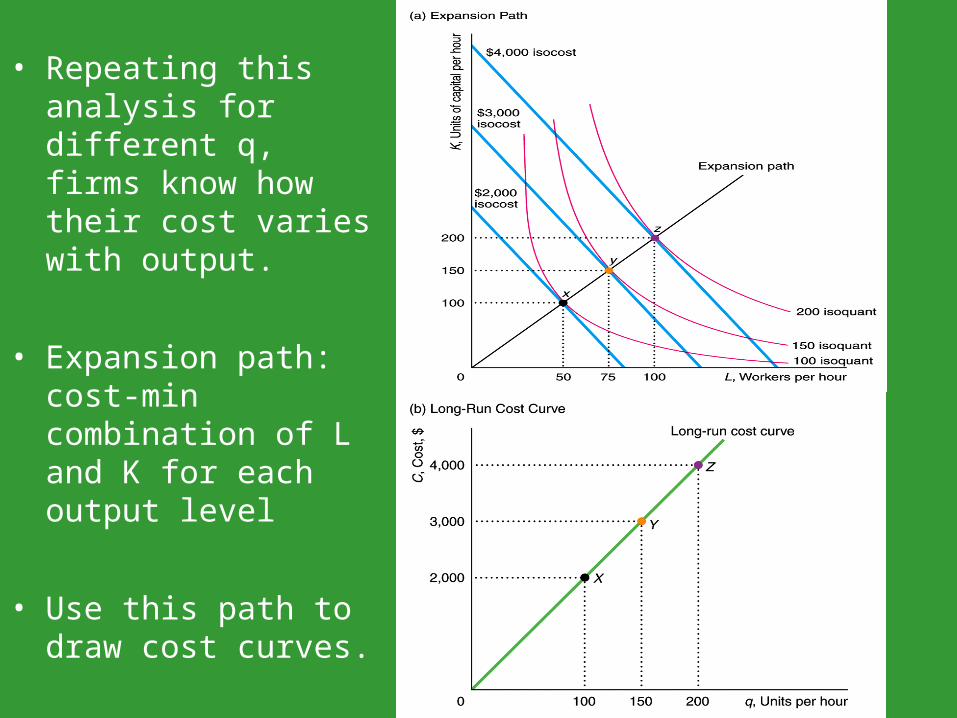
• Repeating this analysis for different q, firms know how their cost varies with output.

• Expansion path: cost-min combination of L and K for each output level

• Use this path to draw cost curves.

• Cost function: C = f(q)– Curve that relates cost of production to output (tells how

much it costs to produce q)

• Cost equation (line): C = wL + rK– w=wage, L=labor, r=rental rate, K=capital.– Shows the total costs of using inputs L and K

• Isocost equation (line): C = wL + rK– All the combinations of inputs that require the same total

expenditure– Similar to budget line in consumer theory

• It is clear that optimum L and K are functions of w, r, and q:L* =L*(w, r, q), K* =K*(w, r, q)

• Substitute L* and K* to the cost equation: C*(w, r, q) = wL*(w, r, q) + rK*(w, r, q),where C* is the cost function, which is derived from the cost minimizing behavior.

• Assuming that factor prices are constant, we often define cost function as C=C(q).

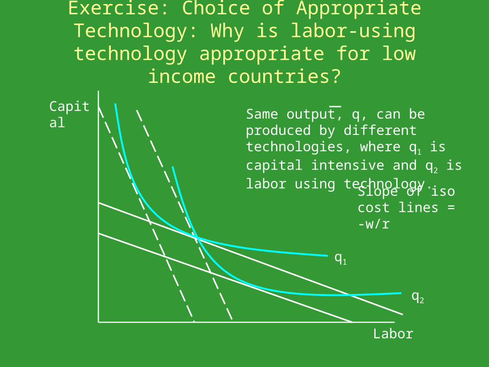
Exercise: Choice of Appropriate Technology: Why is labor-using technology appropriate for

low income countries?

Capital

Labor

Same output, q, can be produced by different technologies, where q1 is capital intensive and q2 is labor using technology.

q1

q2

Slope of isocost lines = -w/r

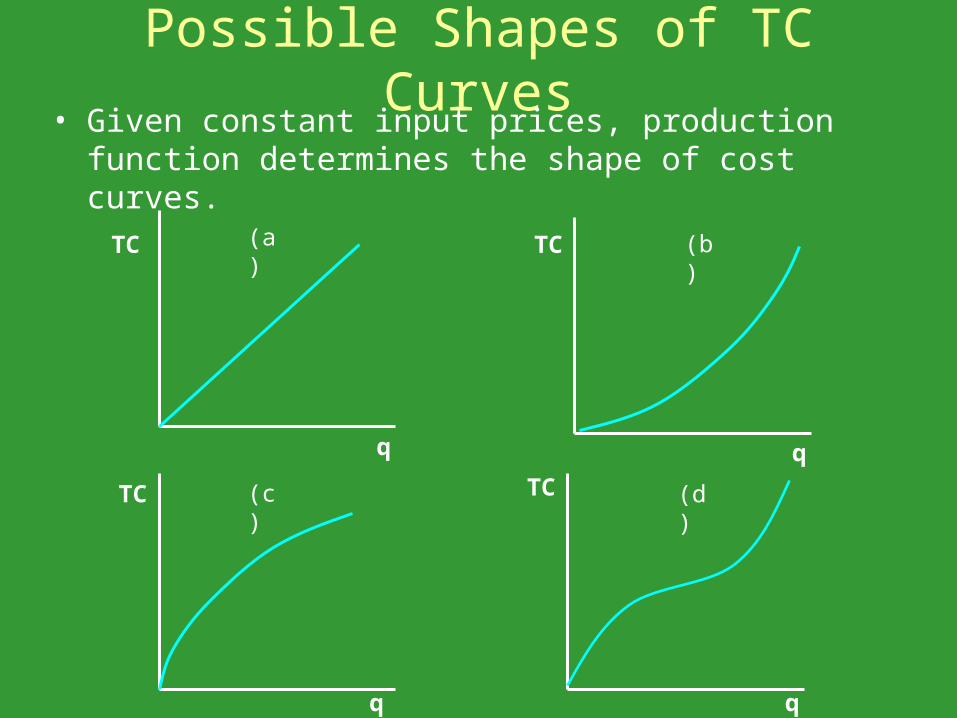
Possible Shapes of TC Curves

TC

TC

TC

TC

q

q

q

q

(a) (b)

(c) (d)

• Given constant input prices, production function determines the shape of cost curves.

Average and Marginal Costs

• Average cost: Total cost per unit of output. Slope of the line from the origin to the corresponding point on the TC.

AC = TC/q

• Marginal Cost: Additional cost of producing one more unit of output. Slope of TC.

MC = dTC/dq

• AC is closely related to returns to scale.

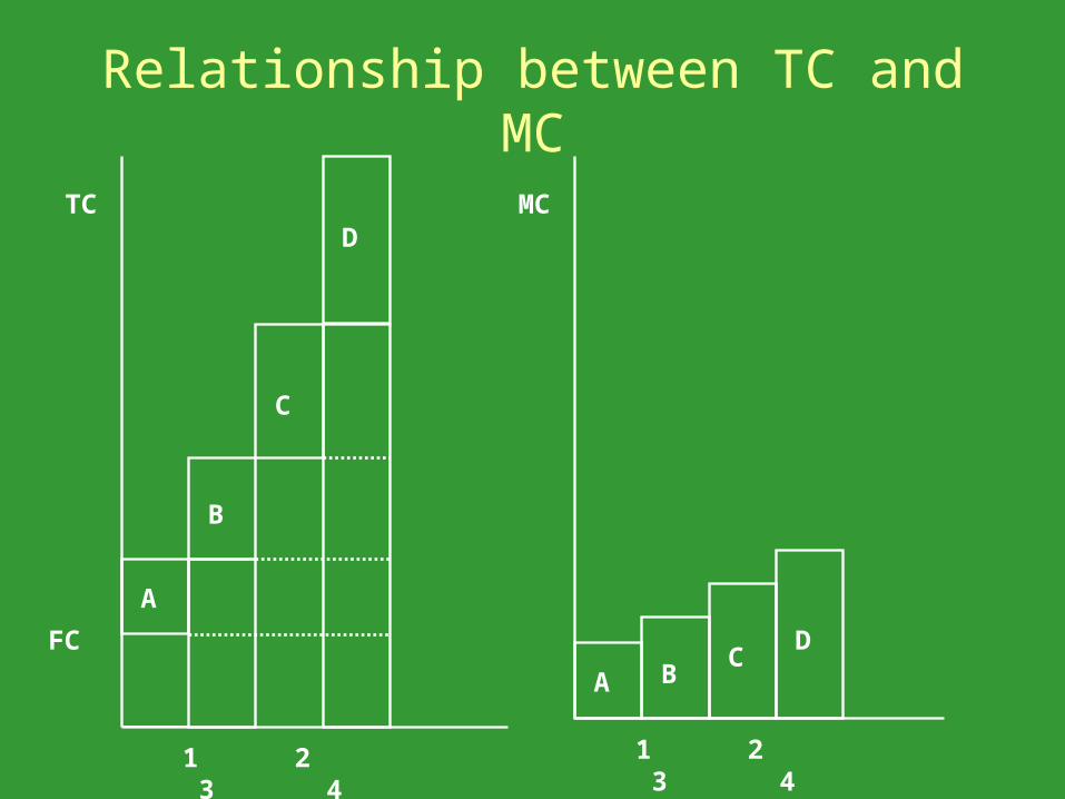
Relationship between TC and MC

TC MC

FC

1 2 3 4 1 2 3 4

A

B

C

D

A BC

D

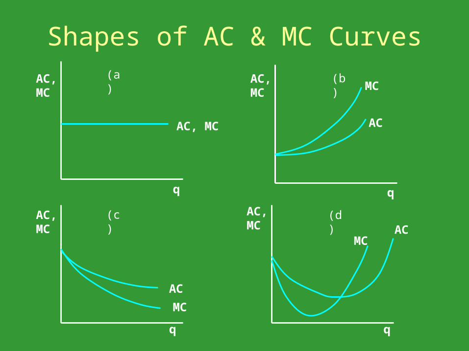
Shapes of AC & MC Curves

AC, MC

AC, MC

AC, MC

AC, MC

q

q

q

q

(a) (b)

(c) (d)

AC

MC

AC

MC

ACMC

AC, MC

Relationship between AC and MC

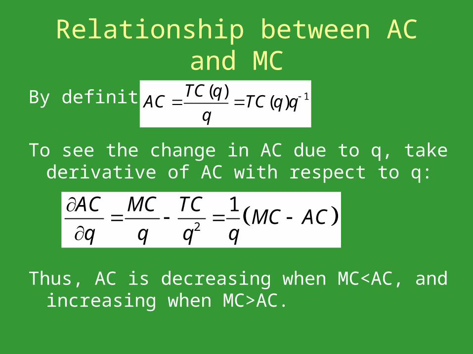
By definition:

To see the change in AC due to q, take derivative of AC with respect to q:

Thus, AC is decreasing when MC<AC, and increasing when MC>AC.

1( )( )

TC qAC TC q q

q

2

1AC MC TCMC AC

q q q q

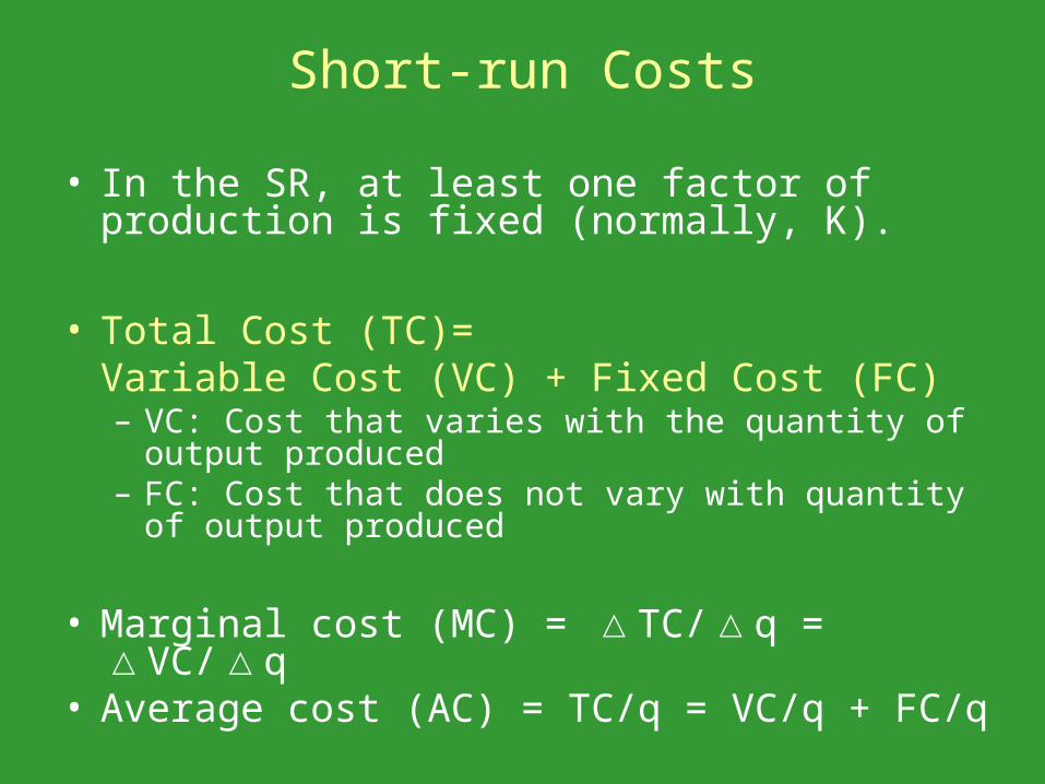
Short-run Costs

• In the SR, at least one factor of production is fixed (normally, K).

• Total Cost (TC)=Variable Cost (VC) + Fixed Cost (FC)

– VC: Cost that varies with the quantity of output produced

– FC: Cost that does not vary with quantity of output produced

• Marginal cost (MC) = TC/ q = VC/ q△ △ △ △• Average cost (AC) = TC/q = VC/q + FC/q

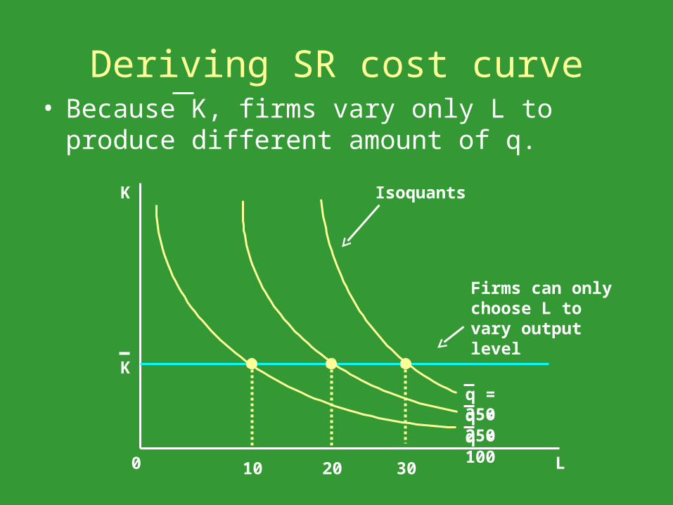
Deriving SR cost curve• Because K, firms vary only L to produce different

amount of q.

K

L

K

q = 100q = 250q = 350

0 10 20 30

Isoquants

Firms can only choose L to vary output level

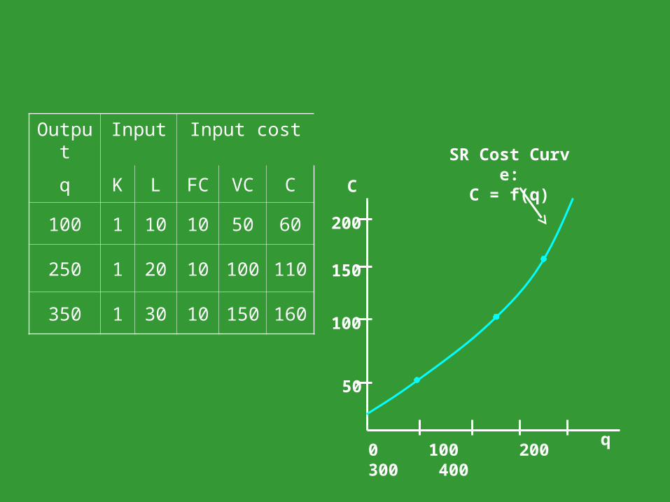
Output Input Input cost

q K L FC VC C

100 1 10 10 50 60

250 1 20 10 100 110

350 1 30 10 150 160

C

q0 100 200 300 400

50

100

150

200

SR Cost Curve:C = f(q)

Shapes of SR Cost Curves

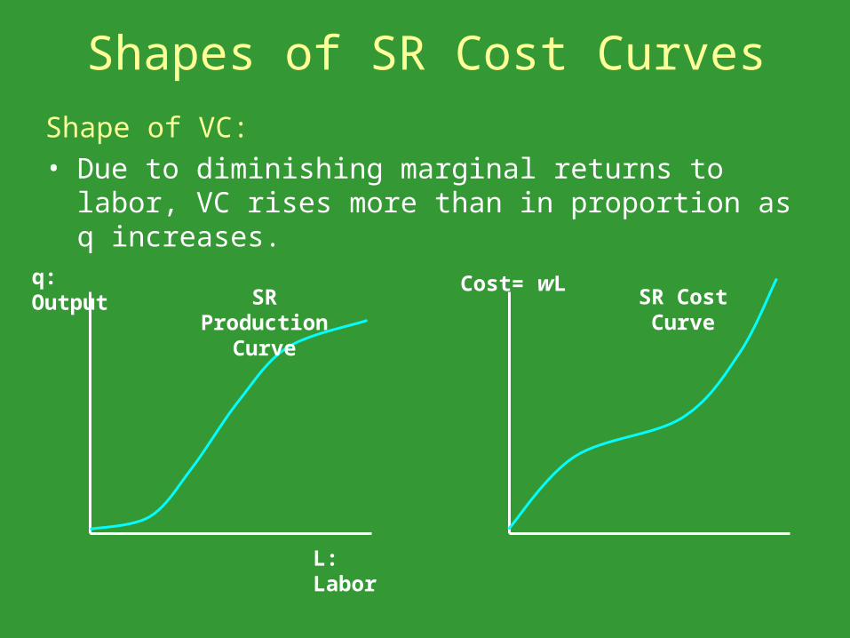
Shape of VC:• Due to diminishing marginal returns to labor, VC rises

more than in proportion as q increases.

Cost= wLSR Cost Curve

q: Output SR Production

Curve

L: Labor

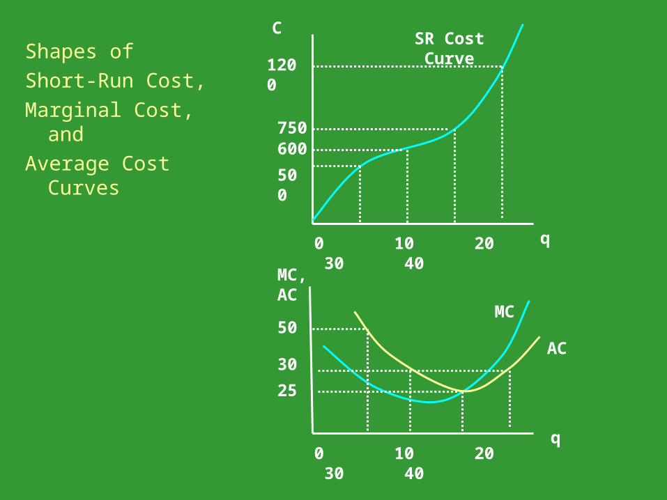
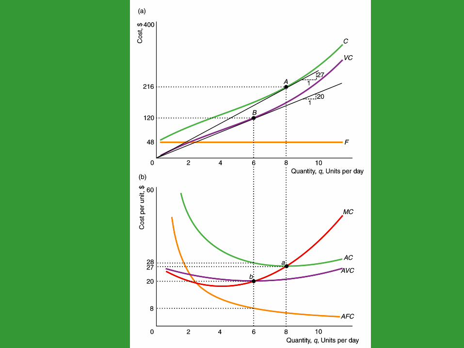
Shapes of

Short-Run Cost,

Marginal Cost, and

Average Cost Curves

C

0 10 20 30 40

500

600750

1200

SR Cost Curve

q

MC, AC

MC

0 10 20 30 40

50

30

25

AC

q

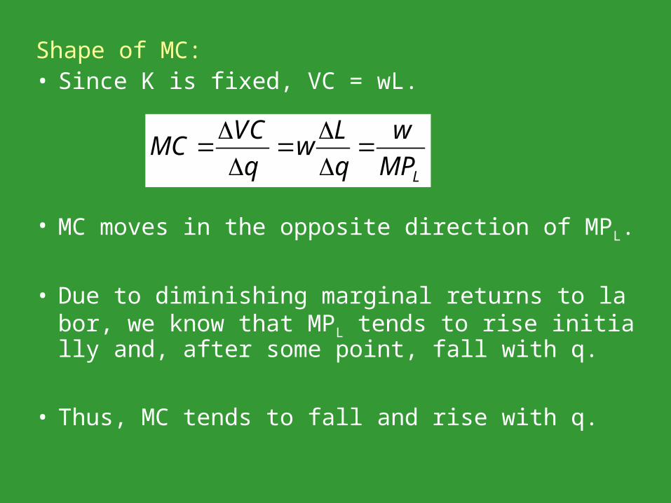
Shape of MC:• Since K is fixed, VC = wL.

• MC moves in the opposite direction of MPL.

• Due to diminishing marginal returns to labor, we know that MPL tends to rise initially and, after some point, fall with q.

• Thus, MC tends to fall and rise with q.

L

VC L wMC w

q q MP

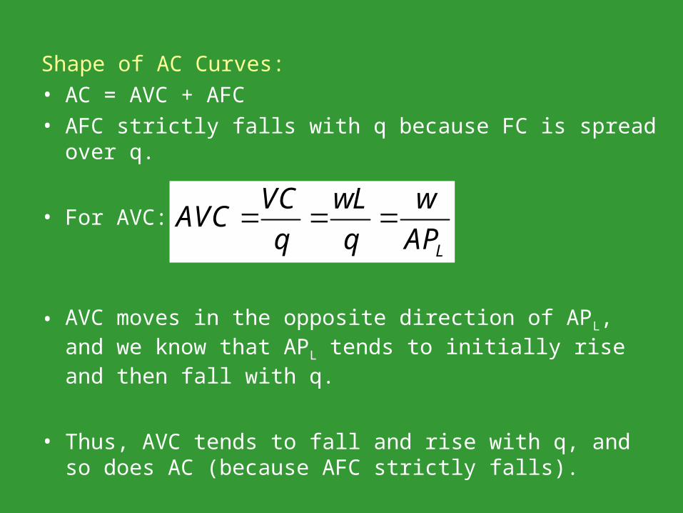
Shape of AC Curves:• AC = AVC + AFC• AFC strictly falls with q because FC is spread over q.

• For AVC:

• AVC moves in the opposite direction of APL, and we know that APL tends to initially rise and then fall with q.

• Thus, AVC tends to fall and rise with q, and so does AC (because AFC strictly falls).

L

VC wL wAVC

q q AP

Lower Costs in the LR

• In the LR planning, firms choose K that minimizes costs given their target output level. In the SR, K is fixed. At some point, firms may invest more in K to produce more efficiently, affecting its SR costs. Thus, LR costs are always equal to or lower than SR costs.

• LRAC connects the lowest point of SRACs that have different levels of K.

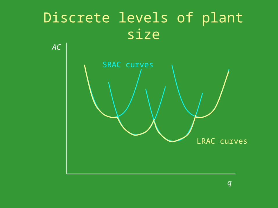
Discrete levels of plant sizeAC

q

SRAC curves

LRAC curves

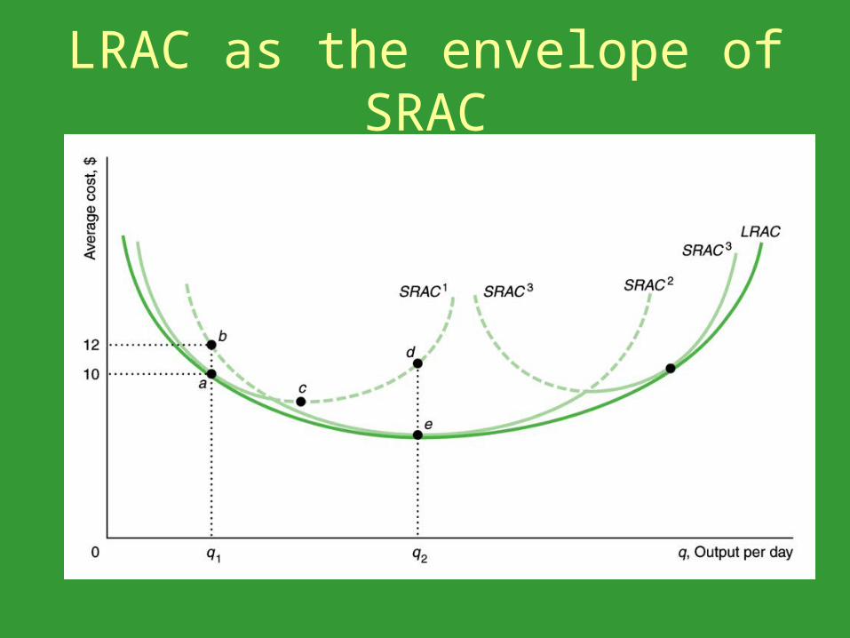
LRAC as the envelope of SRAC

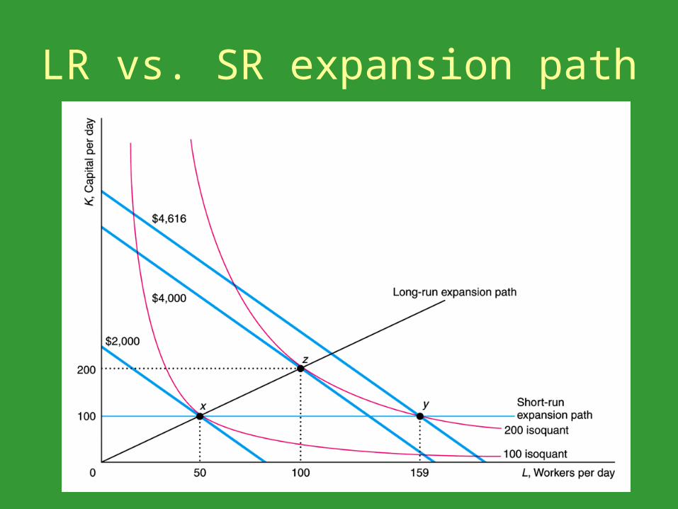
LR vs. SR expansion path

Economies of Scope

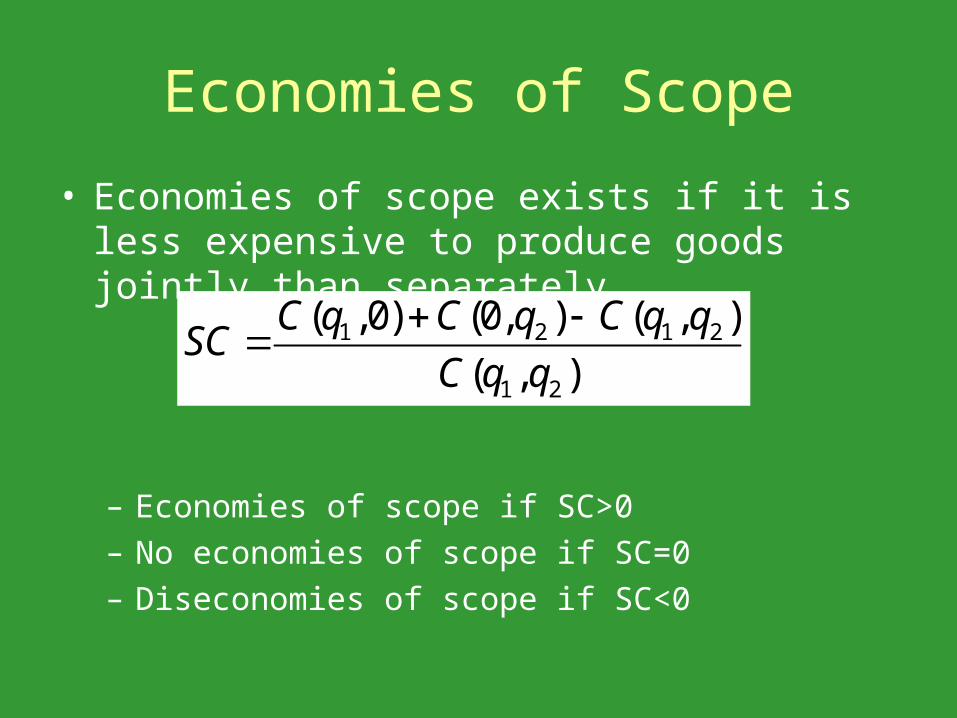
• Economies of scope exists if it is less expensive to produce goods jointly than separately.

– Economies of scope if SC>0– No economies of scope if SC=0– Diseconomies of scope if SC<0

1 2 1 2

1 2

( ,0) (0, ) ( , )

( , )

C q C q C q qSC

C q q

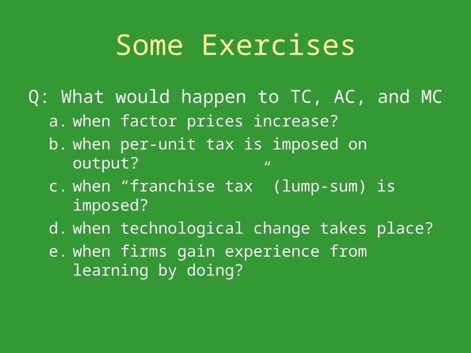
Some Exercises

Q: What would happen to TC, AC, and MCa. when factor prices increase?

b. when per-unit tax is imposed on output?

c. when “franchise tax” (lump-sum) is imposed?

d. when technological change takes place?

e. when firms gain experience from learning by doing?

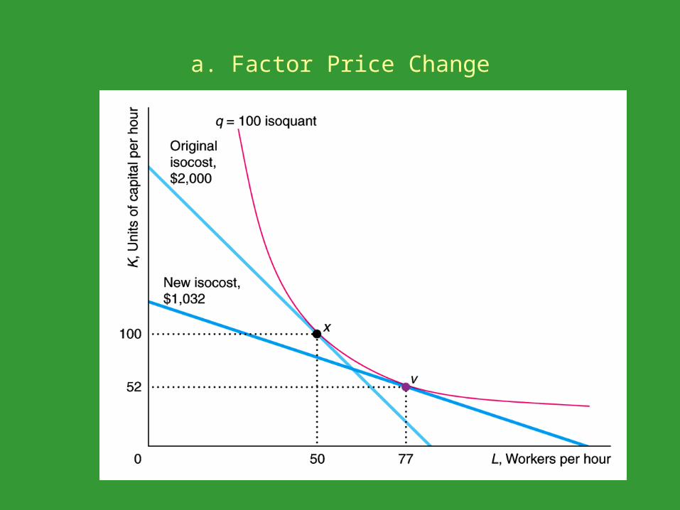
a. Factor Price Change

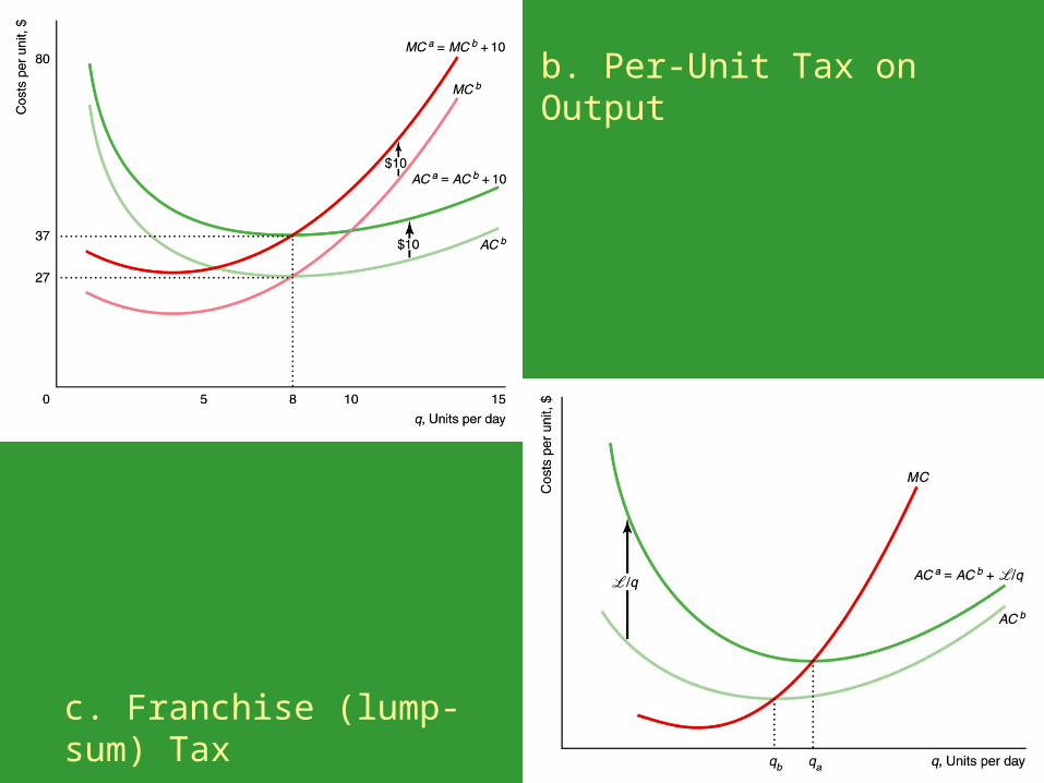
b. Per-Unit Tax on Output

c. Franchise (lump-sum) Tax