Embed Size (px)
Citation preview

Chapter 7
Factorial Analysis of Variance
7.1 Concepts
A factor is just another name for a categorical independent variable. The term is usu-ally used in experimental studies with more than one categorical independent variable,where cases (subjects, patients, experimental units) are randomly assigned to treatmentconditions that represent combinations of the independent variable values. For example,consider an agricultural study in which the cases are plots of land (small fields), the de-pendent variable is crop yield in kilograms, and the independent variables are fertilizertype (three values) and type of irrigation (Sprinkler versus Drip). Table 7.1 shows thesix treatment combinations, one for each cell of the table.
Table 7.1: A Two-Factor Design
Fertilizer 1 Fertilizer 2 Fertilizer 3Sprinker IrrigationDrip Irrigation
Table 7.1 is an example of a complete factorial design, in which data are collected for allcombinations of the independent variable values. In an incomplete, or frational factorialdesign, certain treatment combinations are deliberately omitted, leading to n = 0 in oneor more cells. When done in an organized way1, this practice can save quite a bit ofmoney — say, in a crash test study where the cases are automobiles. In this course, weshall mostly confine our attention to complete factorial designs.
Naturally, a factorial study can have more than two factors. The only limitations areimposed by time and budget. And there is more than one vocabulary floating around2.
1If it is safe to assume that certain contrasts of the treatment means equal zero, it is often possible toestimate and test other contrasts of interest even with zero observations in some cells. The feisibility ofsubstituting assumptions for missing data is an illustration of Data Analysis Hint 4 on page 114.
2This is typical. There are different dialects of Statistics, corresponding roughly to groups of users
166
7.1. CONCEPTS 167
A three-factor design can also be described as a three-way design; there is one “way” foreach dimension of the table of treatment means.
When Sir Ronald Fisher (in whose honour the F -test is named) dreamed up factorialdesigns, he pointed out that they enable the scientist to investigate the effects of severalindependent variables at much less expense than if a separate experiment had to beconducted to test each one. In addition, they allow one to ask systematically whether theeffect of one independent variable depends on the value of another independent variable.If the effect of one independent variable depends on another, we will say there is aninteraction between those variables. This kind of “it depends” conclusion is a lot easierto see when both factors are systematically varied in the same study. Otherwise, one mighteasily think that the results two studies carried out under somewhat different conditionswere inconsistent with one another. We talk about an A “by” B or A × B interaction.Again, an interaction means “it depends.”
A common beginner’s mistake is to confuse the idea of an interaction between variableswith the idea of a relationship between variables. They are different. Consider a versionof Table 7.1 in which the cases are farms and the study is purely observational. Arelationship between Irrigation Type and Fertilizer Type would mean that farms usingdifferent types of fertilizer tend to use different irrigation systems; in other words, thepercentage of farms using Drip irrigation would not be the same for Fertilizer Types 1, 2and 3. This is something that you might assess with a chi-square test of independence.But an interaction between Irrigation Type and Fertilizer Type would mean that theeffect of Irrigation Type on average crop yield depends on the kind of fertilizer used. Aswe will see, this is equivalent to saying that certain contrasts of the treatment means arenot all equal to zero.
7.1.1 Main Effects and Interactions as Contrasts
Testing for main effects by testing contrasts Table 7.2 is an expanded version ofTable 7.1. In addition to population crop yield for each treatment combination (denotedby µ1 through µ6), it shows marginal means – quantities like µ1+µ4
2, which are obtained
by averaging over rows or columns. If there are differences among marginal means for acategorical independent variable in a two-way (or higher) layout like this, we say thereis a main effect for that variable. Tests for main effects are of great interest; they canindicate whether, averaging over the values of the other categorical independent variablesin the design, whether the independent variable in question is related to the dependentvariable. Note that averaging over the values of other independent variables is not thesame thing as controlling for them, but it can still be very informative.
Notice how any difference between marginal means corresponds to a contrast of thetreatment means. It helps to string out all the combinations of factor levels into one longcategorical independent variable. Let’s call this a combination variable. For the crop yieldexample of Tables 7.1 and 7.2, the combination variable has six values, corresponding to
from different disciples. These groups tend not to talk with one another, and often each one has its owntame experts. So the language they use, since it develops in near isolation, tends to diverge in minorways.
168 CHAPTER 7. FACTORIAL ANALYSIS OF VARIANCE
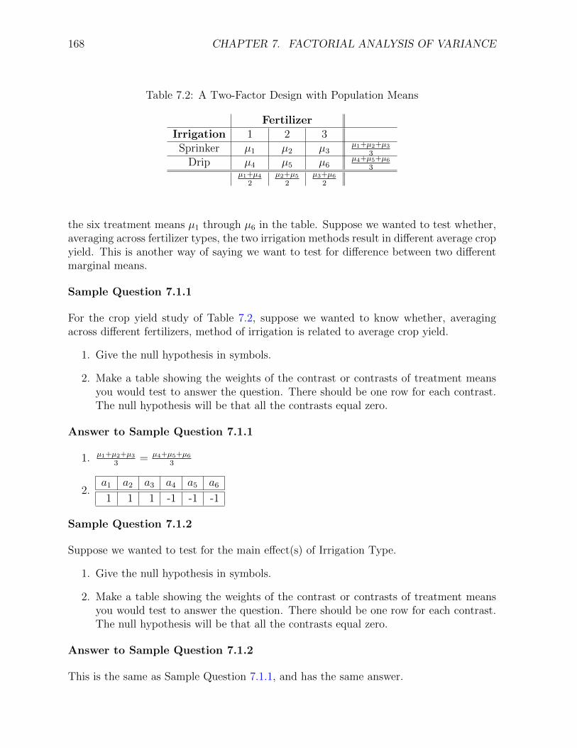
Table 7.2: A Two-Factor Design with Population Means
FertilizerIrrigation 1 2 3
Sprinker µ1 µ2 µ3µ1+µ2+µ3
3
Drip µ4 µ5 µ6µ4+µ5+µ6
3µ1+µ4
2µ2+µ5
2µ3+µ6
2
the six treatment means µ1 through µ6 in the table. Suppose we wanted to test whether,averaging across fertilizer types, the two irrigation methods result in different average cropyield. This is another way of saying we want to test for difference between two differentmarginal means.
Sample Question 7.1.1
For the crop yield study of Table 7.2, suppose we wanted to know whether, averagingacross different fertilizers, method of irrigation is related to average crop yield.
1. Give the null hypothesis in symbols.
2. Make a table showing the weights of the contrast or contrasts of treatment meansyou would test to answer the question. There should be one row for each contrast.The null hypothesis will be that all the contrasts equal zero.
Answer to Sample Question 7.1.1
1. µ1+µ2+µ33
= µ4+µ5+µ63
2.a1 a2 a3 a4 a5 a6
1 1 1 -1 -1 -1
Sample Question 7.1.2
Suppose we wanted to test for the main effect(s) of Irrigation Type.
1. Give the null hypothesis in symbols.
2. Make a table showing the weights of the contrast or contrasts of treatment meansyou would test to answer the question. There should be one row for each contrast.The null hypothesis will be that all the contrasts equal zero.
Answer to Sample Question 7.1.2
This is the same as Sample Question 7.1.1, and has the same answer.
7.1. CONCEPTS 169
Sample Question 7.1.3
Suppose we wanted to know whether, averaging across different methods of irrigation,type of fertilizer is related to average crop yield.
1. Give the null hypothesis in symbols.
2. Make a table showing the weights of the contrast or contrasts of treatment meansyou would test to answer the question. There should be one row for each contrast.The null hypothesis will be that all the contrasts equal zero.
Answer to Sample Question 7.1.3
1. µ1+µ42
= µ2+µ52
= µ3+µ62
2.
a1 a2 a3 a4 a5 a6
1 -1 0 1 -1 00 1 -1 0 1 -1
In the answers to Sample Questions 7.1.1 and 7.1.3, notice that we are testing differ-ences between marginal means, and the number of contrasts is equal to the number ofequals signs in the null hypothesis.
Testing for interactions by testing contrasts Now we will see that tests for inter-actions — that is, tests for whether the effect of a factor depends on the level of anotherfactor — can also be expressed as tests of contrasts. For the crop yield example, considerthis question: Does the effect of Irrigation Type depend on the type of fertilizer used?For Fertilizer Type 1, the effect of Irrigation Type is represented by µ1−µ4. For FertilizerType 2, it is represented by µ2 − µ5, and for Fertilizer Type 2, the effect of IrrigationType is µ3 − µ6. Thus the null hypothesis of no interaction may be written
H0 : µ1 − µ4 = µ2 − µ5 = µ3 − µ6. (7.1)
Because it contains two equals signs, the null hypothesis (7.1) is equivalent to sayingthat two contrasts of the treatment means are equal to zero. Here are the weights of thecontrasts, in tabular form.
a1 a2 a3 a4 a5 a6
1 -1 0 -1 1 00 1 -1 0 -1 1
One way of saying that there is an interaction between Irrigation Method and FertilizerType is to say that the effect of Irrigation Method depends on Fertilizer Type, and nowit is clear how to set up the null hypothesis. But what if the interaction were expressedin the opposite way, by saying that the effect of Fertilizer Type depends on IrrigationMethod? It turns out these two ways of expressing the concept are 100% equivalent.They imply exactly the same null hypothesis, and the significance tests will be identical.
170 CHAPTER 7. FACTORIAL ANALYSIS OF VARIANCE
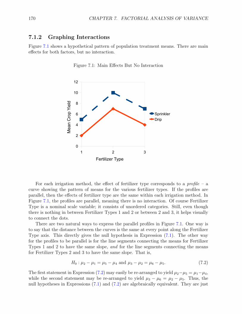
7.1.2 Graphing Interactions
Figure 7.1 shows a hypothetical pattern of population treatment means. There are maineffects for both factors, but no interaction.
Figure 7.1: Main Effects But No Interaction
Sheet1
Page 1
1 2 3Sprinkler 5 10 7Drip 2 7 4
1 2 30
2
4
6
8
10
12
SprinklerDrip
Fertilizer Type
Mea
n C
rop
Yiel
d
For each irrigation method, the effect of fertilizer type corresponds to a profile – acurve showing the pattern of means for the various fertilizer types. If the profiles areparallel, then the effects of fertilizer type are the same within each irrigation method. InFigure 7.1, the profiles are parallel, meaning there is no interaction. Of course FertilizerType is a nominal scale variable; it consists of unordered categories. Still, even thoughthere is nothing in between Fertilizer Types 1 and 2 or between 2 and 3, it helps visuallyto connect the dots.
There are two natural ways to express the parallel profiles in Figure 7.1. One way isto say that the distance between the curves is the same at every point along the FertilizerType axis. This directly gives the null hypothesis in Expression (7.1). The other wayfor the profiles to be parallel is for the line segments connecting the means for FertilizerTypes 1 and 2 to have the same slope, and for the line segments connecting the meansfor Fertilizer Types 2 and 3 to have the same slope. That is,
H0 : µ2 − µ1 = µ5 − µ4 and µ3 − µ2 = µ6 − µ5. (7.2)
The first statement in Expression (7.2) may easily be re-arranged to yield µ2−µ5 = µ1−µ4,while the second statement may be re-arranged to yield µ3 − µ6 = µ2 − µ5. Thus, thenull hypotheses in Expressions (7.1) and (7.2) are algebraically equivalent. They are just
7.1. CONCEPTS 171
different ways of writing the same null hypothesis, and it doesn’t matter which one youuse. Fortunately, this is a very general phenomenon.
7.1.3 Higher order designs (More than two factors)
The extension to more than two factors is straightforward. Suppose that for each com-bination of Irrigation Method and Fertilizer Type, a collection of plots was randomlyassigned to several different types of pesticide (weed killer). Then we would have threefactors: Irrigation Method, Fertilizer Type and Pesticide Type.
• For each independent variable, averaging over the other two variables would givemarginal means – the basis for estimating and testing for main effects. That is,there are three (sets of) main effects: one for Irrigation method, one for Fertilizertype, and one for Pesticide type.
• Averaging over each of the independent variables in turn, we would have a two-waymarginal table of means for the other two variables, and the pattern of means in thattable could show a two-way interaction. That is, there are three 2-facto interactions:Irrigation by Fertilizer, Irrigation by Pesticidde, and Fertilizer by Pesticide.
The full three-dimensional table of means would provide a basis for looking at a three-way, or three-factor interaction. The interpretation of a three-way interaction is thatthe nature of the two-way interaction depends on the value of the third variable. Thisprinciple extends to any number of factors, so we would interpret a six-way interaction tomean that the nature of the 5-way interaction depends on the value of the sixth variable.How would you graph a three-factor interaction? For each value of the third factor, makea separate two-factor plot like Figure 7.1.
Fortunately, the order in which one considers the variables does not matter. Forexample, we can say that the A by B interaction depends on the value of C, or that theA by C interaction depends on B, or that the B by C interaction depends on the valueof A. The translations of these statements into algebra are all equivalent to one another,and lead to exactly the same test statistics and p-values for any set of data, always.
Here are the three ways of describing the three-factor interaction for the Crop Yeldexample.
• The nature of the Irrigation method by Fertilizer type interaction depends on thetype of Pesticide.
• The nature of the Irrigation method by Pesticide type interaction depends on thetype of Fertilizer.
• The nature of the Pesticide type by Fertilizer interaction depends on the Irrigationmethod.
Again, these statements are all equivalent. Use the one that is easiest to think about andtalk about. This principle extends to any number of factors.
172 CHAPTER 7. FACTORIAL ANALYSIS OF VARIANCE
As you might imagine, things get increasingly complicated as the number of factorsbecomes large. For a four-factor design, there are
• Four (sets of) main effects
• Six two-factor interactions
• Four three-factor interactions
• One four-factor interaction; the nature of the three-factor interaction depends onthe value of the 4th factor . . .
• There is an F -test for each one
Also, interpreting higher-way interactions – that is, figuring out what they mean – be-comes more and more difficult for experiments with large numbers of factors. Once I knewa Psychology graduate student who obtained a significant 5-way interaction when she an-alyzed the data for her Ph.D. thesis. Nobody could understand it, so she disappeared fora week. When she came back, she said “I’ve got it!” But nobody could understand herexplanation.
For reasons like this, sometimes the higher-order interactions are deliberately omittedfrom the full model in big experimental designs; they are never tested. Is this reasonable?Most of my answers are just elaborate ways to say I don’t know.
Regardless of how many factors we have, or how many levels there are in each factor,one can always form a combination variable – that is, a single categorical independentvariable whose values represent all the combinations of independent variable values in thefactorial design. Then, tests for main effects and interactions appear as test for collectionsof contrasts on the combination variable. This is helpful, for at least three reasons.
1. Thinking of an interaction as a collection of contrasts can really help you understandwhat it means. And especially for big designs, you need all the help you can get.
2. Once you have seen the tests for main effects and interactions as collections ofcontrasts, it is straightforward to compose a test for any collection of effects (orcomponents of an effect) that is of interest.
3. Seeing main effects and interactions in terms of contrasts makes it easy to see howthey can be modified to become Bonferroni or Scheffe follow-ups to an initial signif-icant one-way ANOVA on the combination variable — if you choose to follow thisconservative data analytic strategy.
7.1.4 Effect coding
While it is helpful to think of main effects and interactions in terms of contrasts, thedetails become unpleasant for designs with more than two factors. The combinationvariables become long, and thinking of interactions as collections of differences betweendifferences of differences can give you a headache. An alternative is to use a regression
7.1. CONCEPTS 173
model with dummy variable coding. For almost any regression model with interactionsbetween categorical independent variabls, the easiest dummy variable coding scheme iseffect coding.
Recall from Section 5.6.3 (see page 125) that effect coding is just like indicator dummyvariable coding with an intercept, except that the last category gets a minus one insteadof a zero. For a single categorical independent variable (factor), the regression coefficientsare deviations of the treatment means from the grand mean, or mean of treatment means.Thus, the regression coefficients are exactly the effects as described in standard textbookson the analysis of variance.
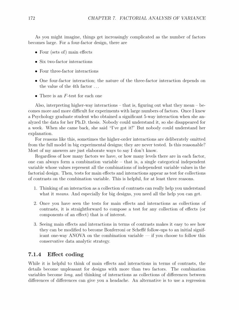
For the two-factor Crop Yield study of Table 7.1 on page 166, here is how the ef-fect coding dummy variables would be defined for Fertiziler type and Irrigation method(Water).
Fertilizer f1 f2
1 1 02 0 13 -1 -1
Water w
Sprinkler 1Drip -1
As in the quantitative by quantitative case (page 133) than the quantitative by cate-gorical case (page 133) the interaction effects are the regression coefficients correspondingto products of independent variables. For a two-factor design, the products come frommultiplying each dummy variable for one factor by each dummy variable for the otherfactor. You never multiply dummy variables for the same factor with each other. Here isthe regression equation for conditional expected crop yield.
E[Y |X] = β0 + β1f1 + β2f2 + β3w + β4f1w + β5f2w
The last two independent variables are quite literally the products of the dummy variablesfor Fertilizer type and Irrigation method.
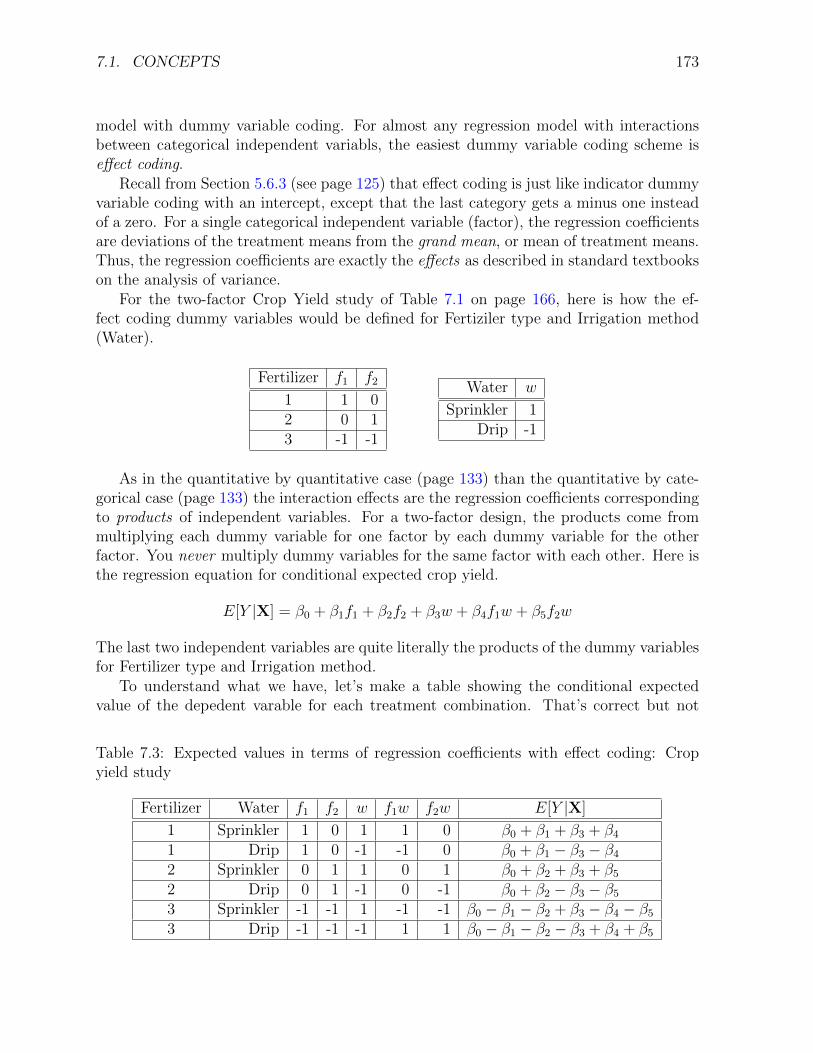
To understand what we have, let’s make a table showing the conditional expectedvalue of the depedent varable for each treatment combination. That’s correct but not
Table 7.3: Expected values in terms of regression coefficients with effect coding: Cropyield study
Fertilizer Water f1 f2 w f1w f2w E[Y |X]
1 Sprinkler 1 0 1 1 0 β0 + β1 + β3 + β41 Drip 1 0 -1 -1 0 β0 + β1 − β3 − β42 Sprinkler 0 1 1 0 1 β0 + β2 + β3 + β52 Drip 0 1 -1 0 -1 β0 + β2 − β3 − β53 Sprinkler -1 -1 1 -1 -1 β0 − β1 − β2 + β3 − β4 − β53 Drip -1 -1 -1 1 1 β0 − β1 − β2 − β3 + β4 + β5
174 CHAPTER 7. FACTORIAL ANALYSIS OF VARIANCE
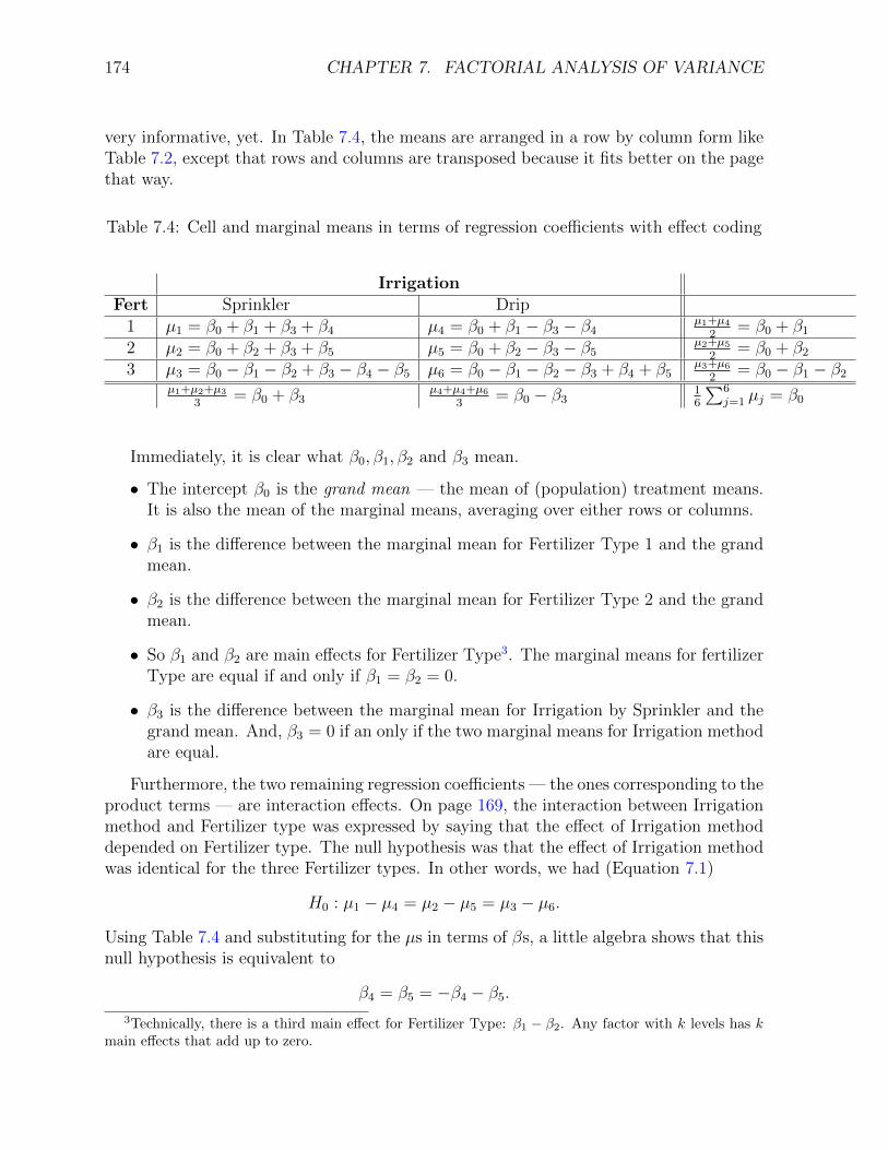
very informative, yet. In Table 7.4, the means are arranged in a row by column form likeTable 7.2, except that rows and columns are transposed because it fits better on the pagethat way.
Table 7.4: Cell and marginal means in terms of regression coefficients with effect coding
IrrigationFert Sprinkler Drip
1 µ1 = β0 + β1 + β3 + β4 µ4 = β0 + β1 − β3 − β4 µ1+µ42
= β0 + β12 µ2 = β0 + β2 + β3 + β5 µ5 = β0 + β2 − β3 − β5 µ2+µ5
2= β0 + β2
3 µ3 = β0 − β1 − β2 + β3 − β4 − β5 µ6 = β0 − β1 − β2 − β3 + β4 + β5µ3+µ6
2= β0 − β1 − β2
µ1+µ2+µ33
= β0 + β3µ4+µ4+µ6
3= β0 − β3 1
6
∑6j=1 µj = β0
Immediately, it is clear what β0, β1, β2 and β3 mean.
• The intercept β0 is the grand mean — the mean of (population) treatment means.It is also the mean of the marginal means, averaging over either rows or columns.
• β1 is the difference between the marginal mean for Fertilizer Type 1 and the grandmean.
• β2 is the difference between the marginal mean for Fertilizer Type 2 and the grandmean.
• So β1 and β2 are main effects for Fertilizer Type3. The marginal means for fertilizerType are equal if and only if β1 = β2 = 0.
• β3 is the difference between the marginal mean for Irrigation by Sprinkler and thegrand mean. And, β3 = 0 if an only if the two marginal means for Irrigation methodare equal.
Furthermore, the two remaining regression coefficients — the ones corresponding to theproduct terms — are interaction effects. On page 169, the interaction between Irrigationmethod and Fertilizer type was expressed by saying that the effect of Irrigation methoddepended on Fertilizer type. The null hypothesis was that the effect of Irrigation methodwas identical for the three Fertilizer types. In other words, we had (Equation 7.1)
H0 : µ1 − µ4 = µ2 − µ5 = µ3 − µ6.
Using Table 7.4 and substituting for the µs in terms of βs, a little algebra shows that thisnull hypothesis is equivalent to
β4 = β5 = −β4 − β5.3Technically, there is a third main effect for Fertilizer Type: β1 − β2. Any factor with k levels has k
main effects that add up to zero.
7.1. CONCEPTS 175
This, in turn, is equivalent to saying that β4 = β5 = 0. So to test for an interaction, wejust test whether the regression coefficients for the product terms equal zero.
General Rules Everything in this example generalizes nicely to an arbitrary numberof factors.
• The regression model has an intercept.
• Define effect coding dummy variables for each factor. If the factor has k levels, therewill be k−1 dummy variables. Each dummy variable has a one for one of the factorlevels, minus one for the last level, and zero for the rest.
• Form new independent variables that are products of the dummy variables. Forany pair of factors A and B, multiply each dummy variable for A by each dummyvariable for B.
• If there are more than two factors, form all three-way products, 4-way products,and so on.
• It’s not hard to get all the products for a multifactor design without missing any.After you have calculated all the products for factors A and B, take the dummyvariables for factor C and
– Multiply each dummy variable for C by each dummy variable for A. Theseproducts correspond to the A× C interaction.
– Multiply each dummy variable for C by each dummy variable for B. Theseproducts correspond to the B × C interaction.
– Multiply each dummy variable for C by each A × B product. These three-variable products correspond to the A×B × C interaction.
• It is straightforward to extend the process, multiplying each dummy variable for afourth factor D by the dummy variables and products in the A × B × C set. Andso on there.
• To test main effects (differences between marginal means) for a factor, the nullhypothesis is that the regression coefficients for that factor’s dummy variables areall equal to zero.
• For any two-factor interaction, test the regression coefficients corresponding to thetwo-way products. For three-factor interactions, test the three-way products, andso on.
• Quantitative covariates may be included in the model, with or without interactionsbetween covariates, or between covariates and factors. They work as expected.Multi-factor analysis of covariance is just a big multiple regression model.
176 CHAPTER 7. FACTORIAL ANALYSIS OF VARIANCE
7.2 Two-factor ANOVA with SAS: The Potato Data
This was covered in class.
7.3 Another example: The Greenhouse Study
This is an extension of the tubes example (see page 77) of Section 3.3. The seeds of thecanola plant yield a high-quality cooking oil. Canola is one of Canada’s biggest cash crops.But each year, millions of dollars are lost because of a fungus that kills canola plants.Or is it just one fungus? All this stuff looks the same. It’s a nasty black rot that growsfastest under moist, warm conditions. It looks quite a bit like the fungus that grows inbetween shower tiles.
A team of botanists recognized that although the fungus may look the same, there areactually several different kinds that are genetically distinct. There are also quite a fewstrains of canola plant, so the questions arose
• Are some strains of fungus more aggressive than others? That is, do they growfaster and overwhelm the plant’s defenses faster?
• Are some strains of canola plant more vulnerable to infection than others?
• Are some strains of fungus more dangerous to certain strains of plant and lessdangerous to others?
These questions can be answered directly by looking at main effects and the inter-action, so a factorial experiment was designed in which canola plants of three differentvarieties were randomly selected to be infected with one of six genetically different typesof fungus. The way they did it was to scrape a little patch at the base of the plant, andwrap the wound with a moist band-aid that had some fungus on it. Then the plant wasplaced in a very moist dark environment for three days. After three days the bandage wasremoved and the plant was put in a commercial greenhouse. On each of 14 consecutivedays, various measurements were made on the plant. Here, we will be concerned withlesion length, the length of the fungus patch on the plant, measured in millimeters.
The dependent variable will be mean lesion length; the mean is over the 14 dailylesion length measurements for each plant. The independent variables are Cultivar (typeof canola plant) and MCG (type of fungus). Type of plant is called cultivar because thefungus grows (is ”cultivated”) on the plant. MCG stands for “Mycelial CompatibilityGroup.” This strange name comes from the way that the botanists decided whether twotypes of fungus were genetically distinct. The would grow two samples on the samedish in a nutrient solution, and if the two fungus patches stayed separate, they weregenetically different. If they grew together into a single patch of fungus (that is, theywere compatible), then they were genetically identical. Apparently, this phenomenon iswell established.
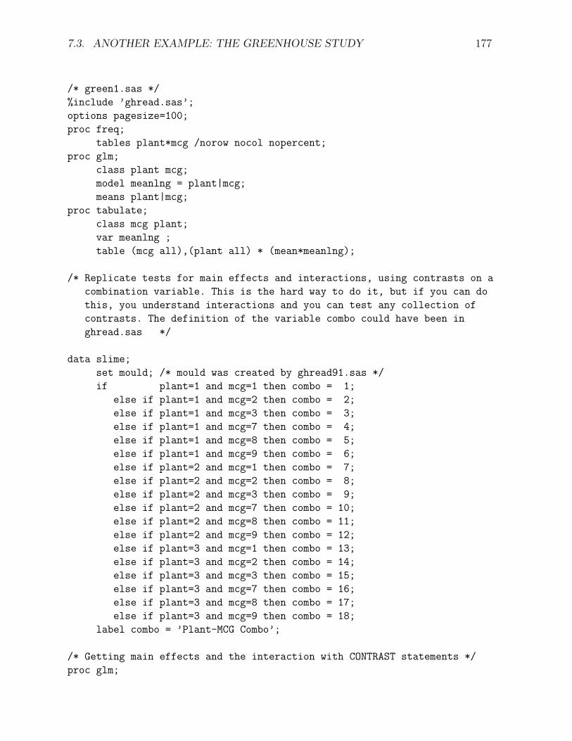
Here is the SAS program green1.sas. As usual, the entire program is listed first.Then pieces of the program are repeated, together with pieces of output and discussion.
7.3. ANOTHER EXAMPLE: THE GREENHOUSE STUDY 177
/* green1.sas */
%include ’ghread.sas’;
options pagesize=100;
proc freq;
tables plant*mcg /norow nocol nopercent;
proc glm;
class plant mcg;
model meanlng = plant|mcg;
means plant|mcg;
proc tabulate;
class mcg plant;
var meanlng ;
table (mcg all),(plant all) * (mean*meanlng);
/* Replicate tests for main effects and interactions, using contrasts on a
combination variable. This is the hard way to do it, but if you can do
this, you understand interactions and you can test any collection of
contrasts. The definition of the variable combo could have been in
ghread.sas */
data slime;
set mould; /* mould was created by ghread91.sas */
if plant=1 and mcg=1 then combo = 1;
else if plant=1 and mcg=2 then combo = 2;
else if plant=1 and mcg=3 then combo = 3;
else if plant=1 and mcg=7 then combo = 4;
else if plant=1 and mcg=8 then combo = 5;
else if plant=1 and mcg=9 then combo = 6;
else if plant=2 and mcg=1 then combo = 7;
else if plant=2 and mcg=2 then combo = 8;
else if plant=2 and mcg=3 then combo = 9;
else if plant=2 and mcg=7 then combo = 10;
else if plant=2 and mcg=8 then combo = 11;
else if plant=2 and mcg=9 then combo = 12;
else if plant=3 and mcg=1 then combo = 13;
else if plant=3 and mcg=2 then combo = 14;
else if plant=3 and mcg=3 then combo = 15;
else if plant=3 and mcg=7 then combo = 16;
else if plant=3 and mcg=8 then combo = 17;
else if plant=3 and mcg=9 then combo = 18;
label combo = ’Plant-MCG Combo’;
/* Getting main effects and the interaction with CONTRAST statements */
proc glm;
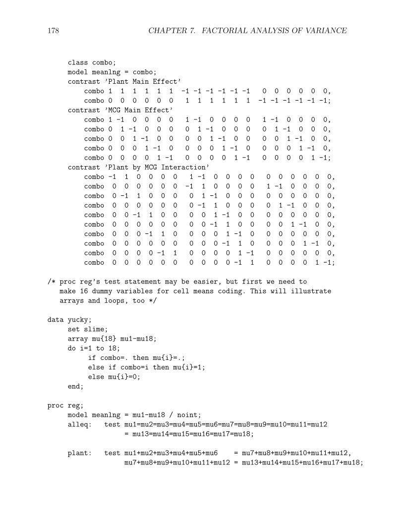
178 CHAPTER 7. FACTORIAL ANALYSIS OF VARIANCE
class combo;
model meanlng = combo;
contrast ’Plant Main Effect’
combo 1 1 1 1 1 1 -1 -1 -1 -1 -1 -1 0 0 0 0 0 0,
combo 0 0 0 0 0 0 1 1 1 1 1 1 -1 -1 -1 -1 -1 -1;
contrast ’MCG Main Effect’
combo 1 -1 0 0 0 0 1 -1 0 0 0 0 1 -1 0 0 0 0,
combo 0 1 -1 0 0 0 0 1 -1 0 0 0 0 1 -1 0 0 0,
combo 0 0 1 -1 0 0 0 0 1 -1 0 0 0 0 1 -1 0 0,
combo 0 0 0 1 -1 0 0 0 0 1 -1 0 0 0 0 1 -1 0,
combo 0 0 0 0 1 -1 0 0 0 0 1 -1 0 0 0 0 1 -1;
contrast ’Plant by MCG Interaction’
combo -1 1 0 0 0 0 1 -1 0 0 0 0 0 0 0 0 0 0,
combo 0 0 0 0 0 0 -1 1 0 0 0 0 1 -1 0 0 0 0,
combo 0 -1 1 0 0 0 0 1 -1 0 0 0 0 0 0 0 0 0,
combo 0 0 0 0 0 0 0 -1 1 0 0 0 0 1 -1 0 0 0,
combo 0 0 -1 1 0 0 0 0 1 -1 0 0 0 0 0 0 0 0,
combo 0 0 0 0 0 0 0 0 -1 1 0 0 0 0 1 -1 0 0,
combo 0 0 0 -1 1 0 0 0 0 1 -1 0 0 0 0 0 0 0,
combo 0 0 0 0 0 0 0 0 0 -1 1 0 0 0 0 1 -1 0,
combo 0 0 0 0 -1 1 0 0 0 0 1 -1 0 0 0 0 0 0,
combo 0 0 0 0 0 0 0 0 0 0 -1 1 0 0 0 0 1 -1;
/* proc reg’s test statement may be easier, but first we need to
make 16 dummy variables for cell means coding. This will illustrate
arrays and loops, too */
data yucky;
set slime;
array mu{18} mu1-mu18;
do i=1 to 18;
if combo=. then mu{i}=.;
else if combo=i then mu{i}=1;
else mu{i}=0;
end;
proc reg;
model meanlng = mu1-mu18 / noint;
alleq: test mu1=mu2=mu3=mu4=mu5=mu6=mu7=mu8=mu9=mu10=mu11=mu12
= mu13=mu14=mu15=mu16=mu17=mu18;
plant: test mu1+mu2+mu3+mu4+mu5+mu6 = mu7+mu8+mu9+mu10+mu11+mu12,
mu7+mu8+mu9+mu10+mu11+mu12 = mu13+mu14+mu15+mu16+mu17+mu18;
7.3. ANOTHER EXAMPLE: THE GREENHOUSE STUDY 179
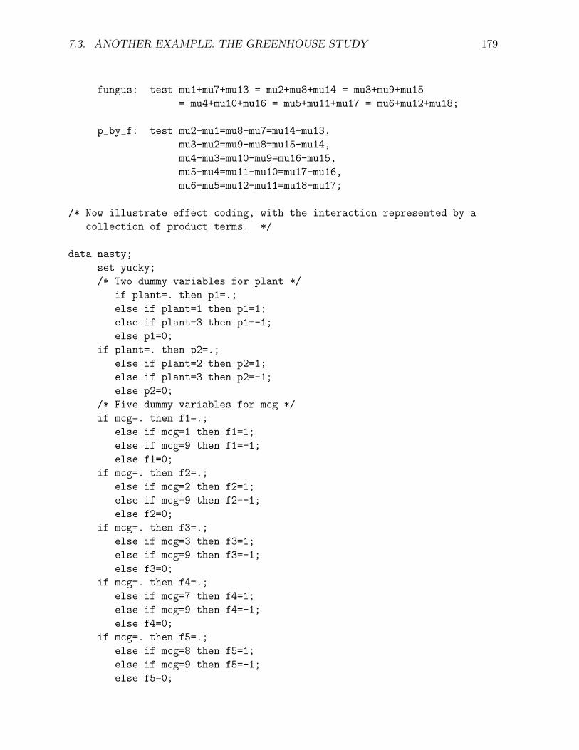
fungus: test mu1+mu7+mu13 = mu2+mu8+mu14 = mu3+mu9+mu15
= mu4+mu10+mu16 = mu5+mu11+mu17 = mu6+mu12+mu18;
p_by_f: test mu2-mu1=mu8-mu7=mu14-mu13,
mu3-mu2=mu9-mu8=mu15-mu14,
mu4-mu3=mu10-mu9=mu16-mu15,
mu5-mu4=mu11-mu10=mu17-mu16,
mu6-mu5=mu12-mu11=mu18-mu17;
/* Now illustrate effect coding, with the interaction represented by a
collection of product terms. */
data nasty;
set yucky;
/* Two dummy variables for plant */
if plant=. then p1=.;
else if plant=1 then p1=1;
else if plant=3 then p1=-1;
else p1=0;
if plant=. then p2=.;
else if plant=2 then p2=1;
else if plant=3 then p2=-1;
else p2=0;
/* Five dummy variables for mcg */
if mcg=. then f1=.;
else if mcg=1 then f1=1;
else if mcg=9 then f1=-1;
else f1=0;
if mcg=. then f2=.;
else if mcg=2 then f2=1;
else if mcg=9 then f2=-1;
else f2=0;
if mcg=. then f3=.;
else if mcg=3 then f3=1;
else if mcg=9 then f3=-1;
else f3=0;
if mcg=. then f4=.;
else if mcg=7 then f4=1;
else if mcg=9 then f4=-1;
else f4=0;
if mcg=. then f5=.;
else if mcg=8 then f5=1;
else if mcg=9 then f5=-1;
else f5=0;
180 CHAPTER 7. FACTORIAL ANALYSIS OF VARIANCE
/* Product terms for interactions */
p1f1 = p1*f1; p1f2=p1*f2 ; p1f3=p1*f3 ; p1f4=p1*f4; p1f5=p1*f5;
p2f1 = p2*f1; p2f2=p2*f2 ; p2f3=p2*f3 ; p2f4=p2*f4; p2f5=p2*f5;
proc reg;
model meanlng = p1 -- p2f5;
plant: test p1=p2=0;
mcg: test f1=f2=f3=f4=f5=0;
p_by_f: test p1f1=p1f2=p1f3=p1f4=p1f5=p2f1=p2f2=p2f3=p2f4=p2f5 = 0;
The SAS program starts with a %include statement that reads ghread.sas. The fileghread.sas consists of a single big data step. We’ll skip it, because all we really need arethe two independent variables plant and mcg, and the dependent variable meanlng.
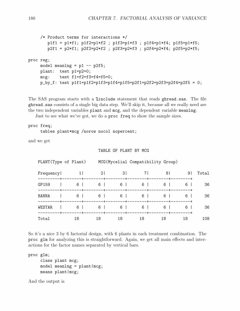
Just to see what we’ve got, we do a proc freq to show the sample sizes.
proc freq;
tables plant*mcg /norow nocol nopercent;
and we get
TABLE OF PLANT BY MCG
PLANT(Type of Plant) MCG(Mycelial Compatibility Group)
Frequency| 1| 2| 3| 7| 8| 9| Total
---------+--------+--------+--------+--------+--------+--------+
GP159 | 6 | 6 | 6 | 6 | 6 | 6 | 36
---------+--------+--------+--------+--------+--------+--------+
HANNA | 6 | 6 | 6 | 6 | 6 | 6 | 36
---------+--------+--------+--------+--------+--------+--------+
WESTAR | 6 | 6 | 6 | 6 | 6 | 6 | 36
---------+--------+--------+--------+--------+--------+--------+
Total 18 18 18 18 18 18 108
So it’s a nice 3 by 6 factorial design, with 6 plants in each treatment combination. Theproc glm for analyzing this is straightforward. Again, we get all main effects and inter-actions for the factor names separated by vertical bars.
proc glm;
class plant mcg;
model meanlng = plant|mcg;
means plant|mcg;
And the output is
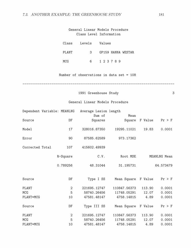
7.3. ANOTHER EXAMPLE: THE GREENHOUSE STUDY 181
General Linear Models Procedure
Class Level Information
Class Levels Values
PLANT 3 GP159 HANNA WESTAR
MCG 6 1 2 3 7 8 9
Number of observations in data set = 108
-------------------------------------------------------------------------------
1991 Greenhouse Study 3
General Linear Models Procedure
Dependent Variable: MEANLNG Average Lesion length
Sum of Mean
Source DF Squares Square F Value Pr > F
Model 17 328016.87350 19295.11021 19.83 0.0001
Error 90 87585.62589 973.17362
Corrected Total 107 415602.49939
R-Square C.V. Root MSE MEANLNG Mean
0.789256 48.31044 31.195731 64.573479
Source DF Type I SS Mean Square F Value Pr > F
PLANT 2 221695.12747 110847.56373 113.90 0.0001
MCG 5 58740.26456 11748.05291 12.07 0.0001
PLANT*MCG 10 47581.48147 4758.14815 4.89 0.0001
Source DF Type III SS Mean Square F Value Pr > F
PLANT 2 221695.12747 110847.56373 113.90 0.0001
MCG 5 58740.26456 11748.05291 12.07 0.0001
PLANT*MCG 10 47581.48147 4758.14815 4.89 0.0001
182 CHAPTER 7. FACTORIAL ANALYSIS OF VARIANCE
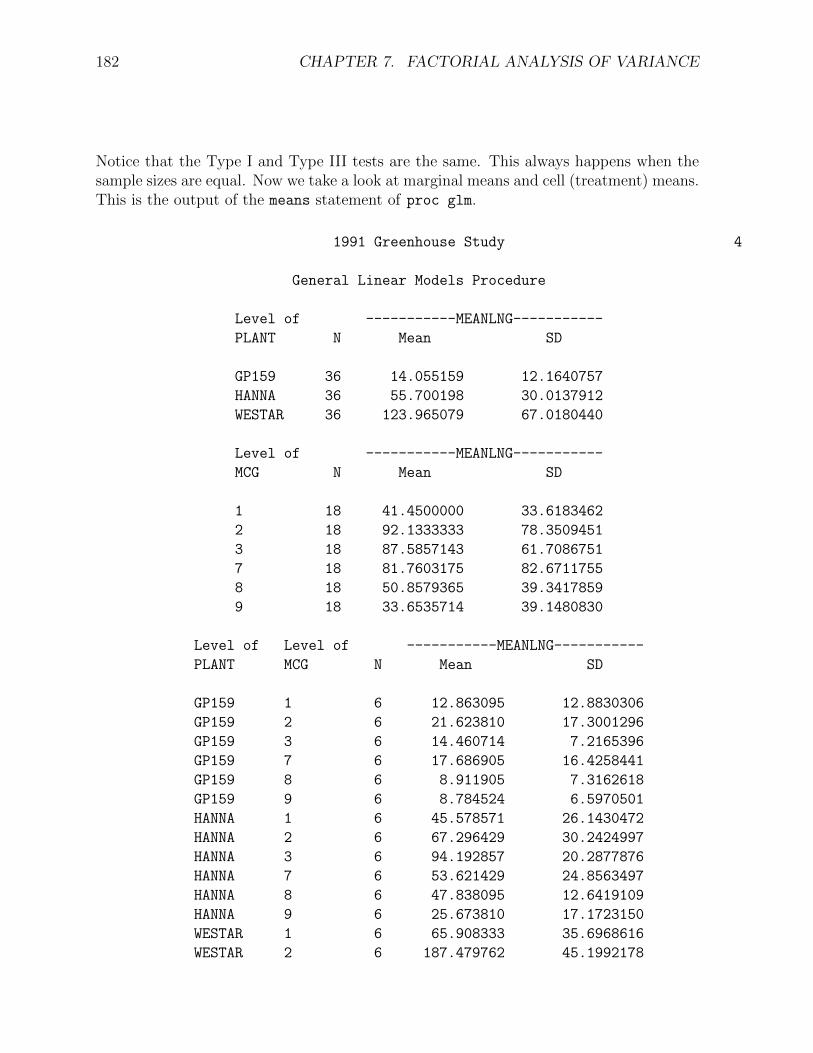
Notice that the Type I and Type III tests are the same. This always happens when thesample sizes are equal. Now we take a look at marginal means and cell (treatment) means.This is the output of the means statement of proc glm.
1991 Greenhouse Study 4
General Linear Models Procedure
Level of -----------MEANLNG-----------
PLANT N Mean SD
GP159 36 14.055159 12.1640757
HANNA 36 55.700198 30.0137912
WESTAR 36 123.965079 67.0180440
Level of -----------MEANLNG-----------
MCG N Mean SD
1 18 41.4500000 33.6183462
2 18 92.1333333 78.3509451
3 18 87.5857143 61.7086751
7 18 81.7603175 82.6711755
8 18 50.8579365 39.3417859
9 18 33.6535714 39.1480830
Level of Level of -----------MEANLNG-----------
PLANT MCG N Mean SD
GP159 1 6 12.863095 12.8830306
GP159 2 6 21.623810 17.3001296
GP159 3 6 14.460714 7.2165396
GP159 7 6 17.686905 16.4258441
GP159 8 6 8.911905 7.3162618
GP159 9 6 8.784524 6.5970501
HANNA 1 6 45.578571 26.1430472
HANNA 2 6 67.296429 30.2424997
HANNA 3 6 94.192857 20.2877876
HANNA 7 6 53.621429 24.8563497
HANNA 8 6 47.838095 12.6419109
HANNA 9 6 25.673810 17.1723150
WESTAR 1 6 65.908333 35.6968616
WESTAR 2 6 187.479762 45.1992178
7.3. ANOTHER EXAMPLE: THE GREENHOUSE STUDY 183
WESTAR 3 6 154.103571 26.5469183
WESTAR 7 6 173.972619 79.1793105
WESTAR 8 6 95.823810 22.3712022
WESTAR 9 6 66.502381 52.5253101
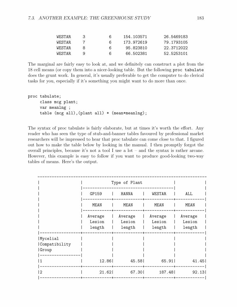
The marginal are fairly easy to look at, and we definitely can construct a plot from the18 cell means (or copy them into a nicer-looking table. But the following proc tabulate
does the grunt work. In general, it’s usually preferable to get the computer to do clericaltasks for you, especially if it’s something you might want to do more than once.
proc tabulate;
class mcg plant;
var meanlng ;
table (mcg all),(plant all) * (mean*meanlng);
The syntax of proc tabulate is fairly elaborate, but at times it’s worth the effort. Anyreader who has seen the type of stub-and-banner tables favoured by professional marketresearchers will be impressed to hear that proc tabulate can come close to that. I figuredout how to make the table below by looking in the manual. I then promptly forgot theoverall principles, because it’s not a tool I use a lot – and the syntax is rather arcane.However, this example is easy to follow if you want to produce good-looking two-waytables of means. Here’s the output.
-----------------------------------------------------------------------
| | Type of Plant | |
| |--------------------------------------| |
| | GP159 | HANNA | WESTAR | ALL |
| |------------+------------+------------+------------|
| | MEAN | MEAN | MEAN | MEAN |
| |------------+------------+------------+------------|
| | Average | Average | Average | Average |
| | Lesion | Lesion | Lesion | Lesion |
| | length | length | length | length |
|-----------------+------------+------------+------------+------------|
|Mycelial | | | | |
|Compatibility | | | | |
|Group | | | | |
|-----------------| | | | |
|1 | 12.86| 45.58| 65.91| 41.45|
|-----------------+------------+------------+------------+------------|
|2 | 21.62| 67.30| 187.48| 92.13|
|-----------------+------------+------------+------------+------------|
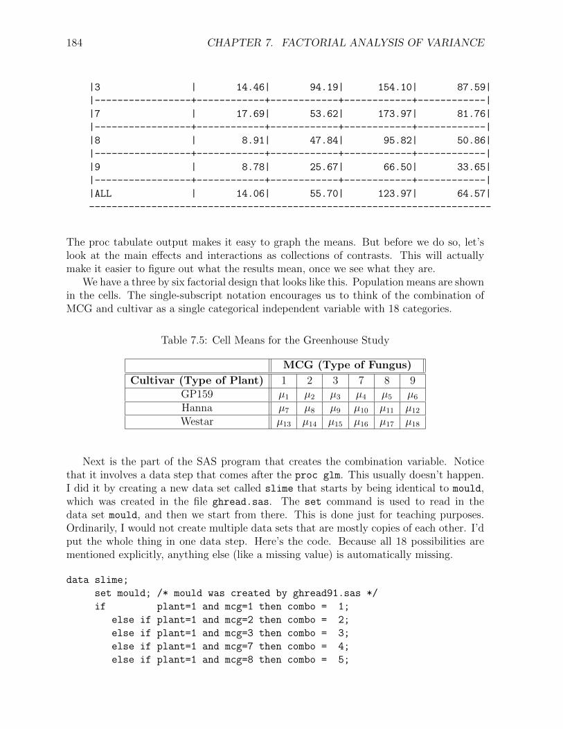
184 CHAPTER 7. FACTORIAL ANALYSIS OF VARIANCE
|3 | 14.46| 94.19| 154.10| 87.59|
|-----------------+------------+------------+------------+------------|
|7 | 17.69| 53.62| 173.97| 81.76|
|-----------------+------------+------------+------------+------------|
|8 | 8.91| 47.84| 95.82| 50.86|
|-----------------+------------+------------+------------+------------|
|9 | 8.78| 25.67| 66.50| 33.65|
|-----------------+------------+------------+------------+------------|
|ALL | 14.06| 55.70| 123.97| 64.57|
-----------------------------------------------------------------------
The proc tabulate output makes it easy to graph the means. But before we do so, let’slook at the main effects and interactions as collections of contrasts. This will actuallymake it easier to figure out what the results mean, once we see what they are.
We have a three by six factorial design that looks like this. Population means are shownin the cells. The single-subscript notation encourages us to think of the combination ofMCG and cultivar as a single categorical independent variable with 18 categories.
Table 7.5: Cell Means for the Greenhouse Study
MCG (Type of Fungus)
Cultivar (Type of Plant) 1 2 3 7 8 9GP159 µ1 µ2 µ3 µ4 µ5 µ6
Hanna µ7 µ8 µ9 µ10 µ11 µ12
Westar µ13 µ14 µ15 µ16 µ17 µ18
Next is the part of the SAS program that creates the combination variable. Noticethat it involves a data step that comes after the proc glm. This usually doesn’t happen.I did it by creating a new data set called slime that starts by being identical to mould,which was created in the file ghread.sas. The set command is used to read in thedata set mould, and then we start from there. This is done just for teaching purposes.Ordinarily, I would not create multiple data sets that are mostly copies of each other. I’dput the whole thing in one data step. Here’s the code. Because all 18 possibilities arementioned explicitly, anything else (like a missing value) is automatically missing.
data slime;
set mould; /* mould was created by ghread91.sas */
if plant=1 and mcg=1 then combo = 1;
else if plant=1 and mcg=2 then combo = 2;
else if plant=1 and mcg=3 then combo = 3;
else if plant=1 and mcg=7 then combo = 4;
else if plant=1 and mcg=8 then combo = 5;
7.3. ANOTHER EXAMPLE: THE GREENHOUSE STUDY 185
else if plant=1 and mcg=9 then combo = 6;
else if plant=2 and mcg=1 then combo = 7;
else if plant=2 and mcg=2 then combo = 8;
else if plant=2 and mcg=3 then combo = 9;
else if plant=2 and mcg=7 then combo = 10;
else if plant=2 and mcg=8 then combo = 11;
else if plant=2 and mcg=9 then combo = 12;
else if plant=3 and mcg=1 then combo = 13;
else if plant=3 and mcg=2 then combo = 14;
else if plant=3 and mcg=3 then combo = 15;
else if plant=3 and mcg=7 then combo = 16;
else if plant=3 and mcg=8 then combo = 17;
else if plant=3 and mcg=9 then combo = 18;
label combo = ’Plant-MCG Combo’;
From Table 7.5on page 184, iIt is clear that the absence of a main effect for Cultivar isthe same as.
µ1 +µ2 +µ3 +µ4 +µ5 +µ6 = µ7 +µ8 +µ9 +µ10 +µ11 +µ12 = µ13 +µ14 +µ15 +µ16. (7.3)
There are two equalities here, and they are saying that two contrasts of the eighteen cellmeans are equal to zero. To see why this is true, recall that a contrast of the 18 treatmentmeans is a linear combination of the form
L = a1µ1 + a1µ2 + . . .+ a18µ18,
where the a weights add up to zero. The table below gives the weights of the contrastsdefining the test for the main effect of plant, one set of weights in each row. The first rowcorresponds to the first equals sign in Equation 7.3. It says that
µ1 + µ2 + µ3 + µ4 + µ5 + µ6 − (µ7 + µ8 + µ9 + µ10 + µ11 + µ12) = 0.
The second row corresponds to the first equals sign in Equation 7.3. It says that
µ7 + µ8 + µ9 + µ10 + µ11 + µ12 − (µ13 + µ14 + µ15 +mu16) = 0.
Table 7.6: Weights of the linear combinations for testing a main effect of cultivar
a1 a2 a3 a4 a5 a6 a7 a8 a9 a10 a11 a12 a13 a14 a15 a16 a17 a181 1 1 1 1 1 -1 -1 -1 -1 -1 -1 0 0 0 0 0 00 0 0 0 0 0 1 1 1 1 1 1 -1 -1 -1 -1 -1 -1
Table 7.6 is the basis of the first contrast statement in proc glm. Notice how thecontrasts are separated by commas. Also notice that the variable on which we’re doingcontrasts (combo) has to be repeated for each contrast.
186 CHAPTER 7. FACTORIAL ANALYSIS OF VARIANCE
/* Getting main effects and the interaction with CONTRAST statements */
proc glm;
class combo;
model meanlng = combo;
contrast ’Plant Main Effect’
combo 1 1 1 1 1 1 -1 -1 -1 -1 -1 -1 0 0 0 0 0 0,
combo 0 0 0 0 0 0 1 1 1 1 1 1 -1 -1 -1 -1 -1 -1;
If there is no main effect for MCG, we are saying
µ1+µ7+µ13 = µ2+µ8+µ14 = µ3+µ9+µ15 = µ4+µ10+µ16 = µ5+µ11+µ17 = µ6+µ12+µ18.
There are 5 contrasts here, one for each equals sign; there is always an equals sign foreach contrast. Table 7.7 shows the weights of the contrasts.
Table 7.7: Weights of the linear combinations for testing a main effect of MCG (Fungustype)
a1 a2 a3 a4 a5 a6 a7 a8 a9 a10 a11 a12 a13 a14 a15 a16 a17 a181 -1 0 0 0 0 1 -1 0 0 0 0 1 -1 0 0 0 00 1 -1 0 0 0 0 1 -1 0 0 0 0 1 -1 0 0 00 0 1 -1 0 0 0 0 1 -1 0 0 0 0 1 -1 0 00 0 0 1 -1 0 0 0 0 1 -1 0 0 0 0 1 -1 00 0 0 0 1 -1 0 0 0 0 1 -1 0 0 0 0 1 -1
And here is the corresponding test statement in proc glm.
contrast ’MCG Main Effect’
combo 1 -1 0 0 0 0 1 -1 0 0 0 0 1 -1 0 0 0 0,
combo 0 1 -1 0 0 0 0 1 -1 0 0 0 0 1 -1 0 0 0,
combo 0 0 1 -1 0 0 0 0 1 -1 0 0 0 0 1 -1 0 0,
combo 0 0 0 1 -1 0 0 0 0 1 -1 0 0 0 0 1 -1 0,
combo 0 0 0 0 1 -1 0 0 0 0 1 -1 0 0 0 0 1 -1;
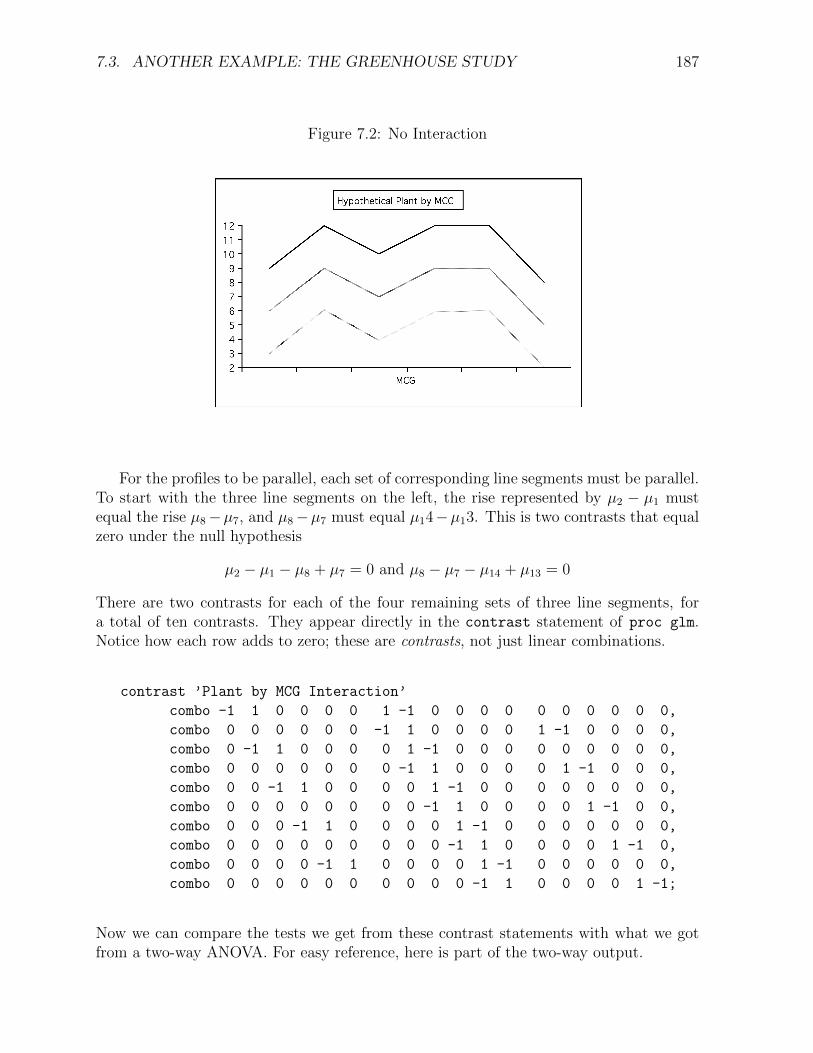
To compose the Plant by MCG interaction, consider the hypothetical graph in Figure 7.2.You can think of the “effect” of MCG as a profile, representing a pattern of differencesamong means. If the three profiles are the same shape for each type of plant – that is, ifthey are parallel, the effect of MCG does not depend on the type of plant, and there isno interaction.
7.3. ANOTHER EXAMPLE: THE GREENHOUSE STUDY 187
Figure 7.2: No Interaction
Chapter 7, Page 47
For the profiles to be parallel, each set of corresponding line segments must be parallel. To start with the three
line segments on the left, the rise represented by µ2−µ1 must equal the rise µ8−µ7, and µ8−µ7 must equal µ14−µ13.
This is two contrasts that equal zero:
µ2 − µ1 – µ8 + µ7 = 0 and µ8−µ7 –µ14+µ13 = 0.
There are two contrasts for each of the four remaining sets of three line segments, for a total of ten contrasts.
They appear directly in the contrast statement of proc glm. Notice how each row adds to zero; these
are contrasts, not just linear combinations.
contrast 'Plant by MCG Interaction'
combo -1 1 0 0 0 0 1 -1 0 0 0 0 0 0 0 0 0 0,
combo 0 0 0 0 0 0 -1 1 0 0 0 0 1 -1 0 0 0 0,
combo 0 -1 1 0 0 0 0 1 -1 0 0 0 0 0 0 0 0 0,
combo 0 0 0 0 0 0 0 -1 1 0 0 0 0 1 -1 0 0 0,
combo 0 0 -1 1 0 0 0 0 1 -1 0 0 0 0 0 0 0 0,
combo 0 0 0 0 0 0 0 0 -1 1 0 0 0 0 1 -1 0 0,
combo 0 0 0 -1 1 0 0 0 0 1 -1 0 0 0 0 0 0 0,
For the profiles to be parallel, each set of corresponding line segments must be parallel.To start with the three line segments on the left, the rise represented by µ2 − µ1 mustequal the rise µ8−µ7, and µ8−µ7 must equal µ14−µ13. This is two contrasts that equalzero under the null hypothesis
µ2 − µ1 − µ8 + µ7 = 0 and µ8 − µ7 − µ14 + µ13 = 0
There are two contrasts for each of the four remaining sets of three line segments, fora total of ten contrasts. They appear directly in the contrast statement of proc glm.Notice how each row adds to zero; these are contrasts, not just linear combinations.
contrast ’Plant by MCG Interaction’
combo -1 1 0 0 0 0 1 -1 0 0 0 0 0 0 0 0 0 0,
combo 0 0 0 0 0 0 -1 1 0 0 0 0 1 -1 0 0 0 0,
combo 0 -1 1 0 0 0 0 1 -1 0 0 0 0 0 0 0 0 0,
combo 0 0 0 0 0 0 0 -1 1 0 0 0 0 1 -1 0 0 0,
combo 0 0 -1 1 0 0 0 0 1 -1 0 0 0 0 0 0 0 0,
combo 0 0 0 0 0 0 0 0 -1 1 0 0 0 0 1 -1 0 0,
combo 0 0 0 -1 1 0 0 0 0 1 -1 0 0 0 0 0 0 0,
combo 0 0 0 0 0 0 0 0 0 -1 1 0 0 0 0 1 -1 0,
combo 0 0 0 0 -1 1 0 0 0 0 1 -1 0 0 0 0 0 0,
combo 0 0 0 0 0 0 0 0 0 0 -1 1 0 0 0 0 1 -1;
Now we can compare the tests we get from these contrast statements with what we gotfrom a two-way ANOVA. For easy reference, here is part of the two-way output.
188 CHAPTER 7. FACTORIAL ANALYSIS OF VARIANCE
Source DF Type III SS Mean Square F Value Pr > F
PLANT 2 221695.12747 110847.56373 113.90 0.0001
MCG 5 58740.26456 11748.05291 12.07 0.0001
PLANT*MCG 10 47581.48147 4758.14815 4.89 0.0001
And here is the output from the contrast statements.
Contrast DF Contrast SS Mean Square F Value Pr > F
Plant Main Effect 2 221695.12747 110847.56373 113.90 0.0001
MCG Main Effect 5 58740.26456 11748.05291 12.07 0.0001
Plant by MCG Interac 10 47581.48147 4758.14815 4.89 0.0001
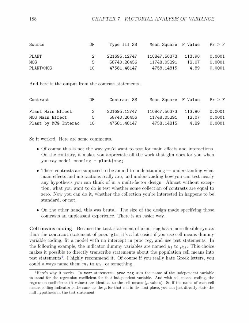
So it worked. Here are some comments.
• Of course this is not the way you’d want to test for main effects and interactions.On the contrary, it makes you appreciate all the work that glm does for you whenyou say model meanlng = plant|mcg;
• These contrasts are supposed to be an aid to understanding — understanding whatmain effects and interactions really are, and understanding how you can test nearlyany hypothesis you can think of in a multi-factor design. Almost without excep-tion, what you want to do is test whether some collection of contrasts are equal tozero. Now you can do it, whether the collection you’re interested in happens to bestandard, or not.
• On the other hand, this was brutal. The size of the design made specifying thosecontrasts an unpleasant experience. There is an easier way.
Cell means coding Because the test statement of proc reg has a more flexible syntaxthan the contrast statement of proc glm, it’s a lot easier if you use cell means dummyvariable coding, fit a model with no intercept in proc reg, and use test statements. Inthe following example, the indicator dummy variables are named µ1 to µ18. This choicemakes it possible to directly transcribe statements about the population cell means intotest statements4. I highly recommend it. Of course if you really hate Greek letters, youcould always name them m1 to m18 or something.
4Here’s why it works. In test statements, proc reg uses the name of the independent variableto stand for the regression coefficient for that independent variable. And with cell means coding, theregression coefficients (β values) are identical to the cell means (µ values). So if the name of each cellmeans coding indicator is the same as the µ for that cell in the first place, you can just directly state thenull hypothesis in the test statement.
7.3. ANOTHER EXAMPLE: THE GREENHOUSE STUDY 189
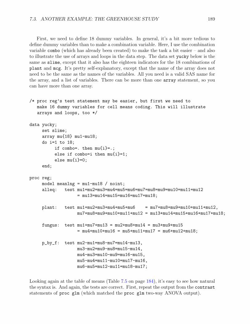
First, we need to define 18 dummy variables. In general, it’s a bit more tedious todefine dummy variables than to make a combination variable. Here, I use the combinationvariable combo (which has already been created) to make the task a bit easier – and alsoto illustrate the use of arrays and loops in the data step. The data set yucky below is thesame as slime, except that it also has the eighteen indicators for the 18 combinations ofplant and mcg. It’s pretty self-explanatory, except that the name of the array does notneed to be the same as the names of the variables. All you need is a valid SAS name forthe array, and a list of variables. There can be more than one array statement, so youcan have more than one array.
/* proc reg’s test statement may be easier, but first we need to
make 16 dummy variables for cell means coding. This will illustrate
arrays and loops, too */
data yucky;
set slime;
array mu{18} mu1-mu18;
do i=1 to 18;
if combo=. then mu{i}=.;
else if combo=i then mu{i}=1;
else mu{i}=0;
end;
proc reg;
model meanlng = mu1-mu18 / noint;
alleq: test mu1=mu2=mu3=mu4=mu5=mu6=mu7=mu8=mu9=mu10=mu11=mu12
= mu13=mu14=mu15=mu16=mu17=mu18;
plant: test mu1+mu2+mu3+mu4+mu5+mu6 = mu7+mu8+mu9+mu10+mu11+mu12,
mu7+mu8+mu9+mu10+mu11+mu12 = mu13+mu14+mu15+mu16+mu17+mu18;
fungus: test mu1+mu7+mu13 = mu2+mu8+mu14 = mu3+mu9+mu15
= mu4+mu10+mu16 = mu5+mu11+mu17 = mu6+mu12+mu18;
p_by_f: test mu2-mu1=mu8-mu7=mu14-mu13,
mu3-mu2=mu9-mu8=mu15-mu14,
mu4-mu3=mu10-mu9=mu16-mu15,
mu5-mu4=mu11-mu10=mu17-mu16,
mu6-mu5=mu12-mu11=mu18-mu17;
Looking again at the table of means (Table 7.5 on page 184), it’s easy to see how naturalthe syntax is. And again, the tests are correct. First, repeat the output from the contraststatements of proc glm (which matched the proc glm two-way ANOVA output).
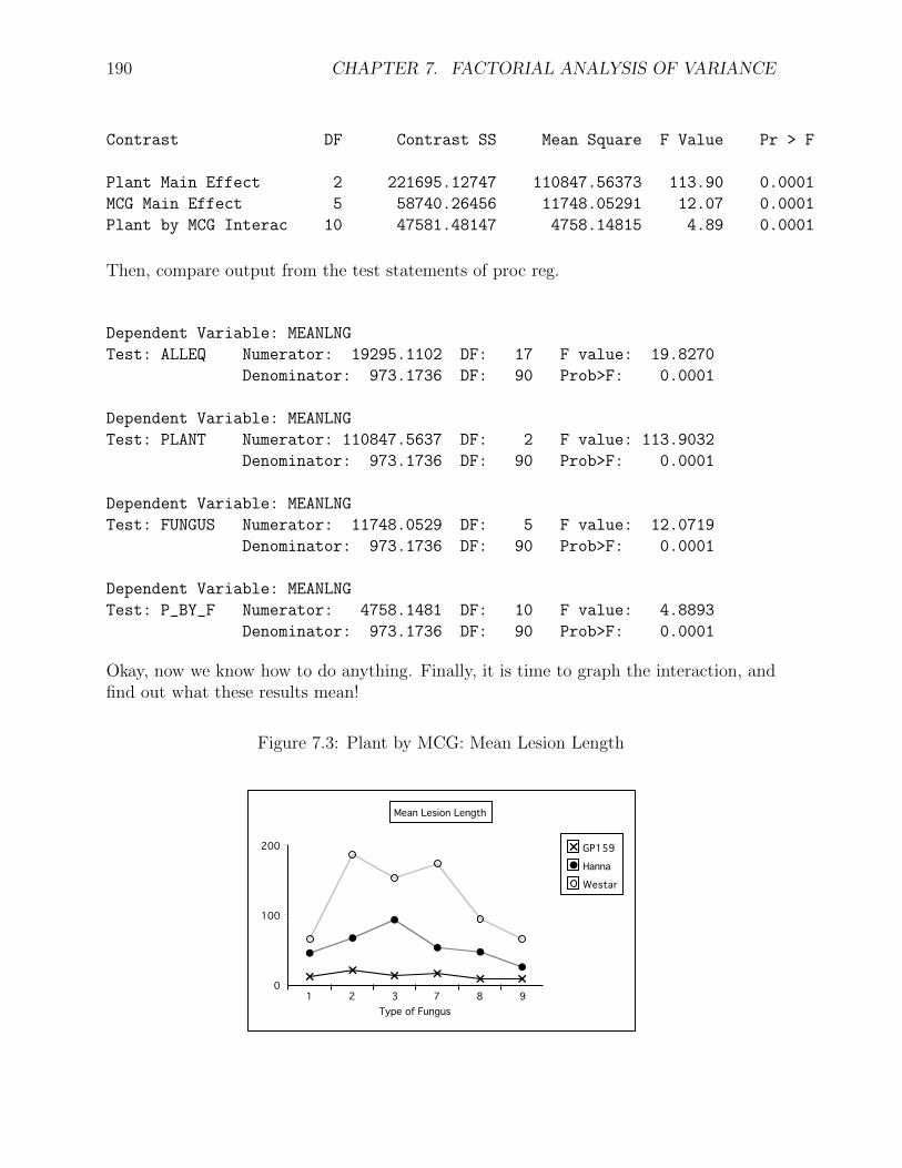
190 CHAPTER 7. FACTORIAL ANALYSIS OF VARIANCE
Contrast DF Contrast SS Mean Square F Value Pr > F
Plant Main Effect 2 221695.12747 110847.56373 113.90 0.0001
MCG Main Effect 5 58740.26456 11748.05291 12.07 0.0001
Plant by MCG Interac 10 47581.48147 4758.14815 4.89 0.0001
Then, compare output from the test statements of proc reg.
Dependent Variable: MEANLNG
Test: ALLEQ Numerator: 19295.1102 DF: 17 F value: 19.8270
Denominator: 973.1736 DF: 90 Prob>F: 0.0001
Dependent Variable: MEANLNG
Test: PLANT Numerator: 110847.5637 DF: 2 F value: 113.9032
Denominator: 973.1736 DF: 90 Prob>F: 0.0001
Dependent Variable: MEANLNG
Test: FUNGUS Numerator: 11748.0529 DF: 5 F value: 12.0719
Denominator: 973.1736 DF: 90 Prob>F: 0.0001
Dependent Variable: MEANLNG
Test: P_BY_F Numerator: 4758.1481 DF: 10 F value: 4.8893
Denominator: 973.1736 DF: 90 Prob>F: 0.0001
Okay, now we know how to do anything. Finally, it is time to graph the interaction, andfind out what these results mean!
Figure 7.3: Plant by MCG: Mean Lesion Length
Chapter 7, Page 52
Denominator: 973.1736 DF: 90 Prob>F: 0.0001
Dependent Variable: MEANLNG
Test: FUNGUS Numerator: 11748.0529 DF: 5 F value: 12.0719
Denominator: 973.1736 DF: 90 Prob>F: 0.0001
Dependent Variable: MEANLNG
Test: P_BY_F Numerator: 4758.1481 DF: 10 F value: 4.8893
Denominator: 973.1736 DF: 90 Prob>F: 0.0001
Okay, now we know how to do anything. Finally, it is time to graph the interaction, and find out what these
results mean!
200
100
0
Type of Fungus1 2 3 7 8 9
Mean Lesion Length
GP159
Hanna
Westar
7.3. ANOTHER EXAMPLE: THE GREENHOUSE STUDY 191
First, we see a sizable and clear main effect for Plant. In fact, going back to theanalysis of variance summary tables and dividing the Sum of Squares explained by Plantby the Total Sum of Squares, we observe that Plant explains around 53 percent of thevariation in mean lesion length. That’s huge. We will definitely want to look at pairwisecomparisons of marginal means, too; we’ll get back to this later.
Looking at the pattern of means, it’s clear that while the main effect of fungus type isstatistically significant, this is not something that should be interpreted, because whichone is best (worst) depends on the type of plant. That is, we need to look at the interac-tion.
Before proceeding I should mention that many text advise us to never interpret maineffects if the interaction is statistically significant. I disagree, and Figure 7.3 is a goodexample of why. It is clear that while the magnitudes of the differences depend on typeof fungus, the lesion lengths are generally largest on Westar and smallest on GP159. Soaveraging over fungus types is a reasonable thing to do.
This does not mean the interaction should be ignored; the three profiles really lookdifferent. In particular, GP159 not only has a smaller average lesion length, but it seemsto exhibit less responsiveness to different strains of fungus. A test for the equality of µ1
through µ6 would be valuable. Pairwise comparisons of the 6 means for Hanna and the 6means for Westar look promising, too.
A Brief Consideration of Multiple Comparisons The mention of pairwise compar-isons brings up the issue of formal multiple comparison follow-up tests for this problem.The way people often do follow-up tests for factorial designs is to make a combinationvariable and then do all pairwise comparisons. It seems like they do this because theythink it’s the only thing the software will let them do. Certainly it’s better than nothing.Here are some comments:
• With SAS, pairwise comparisons of cell means are not the only thing you can do.Proc glm will do all pairwise comparisons of marginal means quite easily. Thismeans it’s easy to follow up a significant and meaningful main effect.
• For the present problem, there are 120 possible pairwise comparisons of the 16 cellmeans. If we do all these as one-at-a-time tests, the chances of false significance arecertainly mounting. There is a strong case here for protectng the tests at a singlejoint significance level.
• Since the sample sizes are equal, Tukey tests are most powerful for all pairwisecomparisons. But it’s not so simple. Pairwise comparisons within plants (for exam-ple, comparing the 6 means for Westar) are interesting, and pairwise comparisonswithin fungus types (for example, comparison of Hanna, Westar and GP159 forfungus Type 1) are interesting, but the remaining 57 pairwise comparisons are a lotless so.
• Also, pairwise comparisons of cell means are not all we want to do. We’ve alreadymentioned the need for pairwise comparisons of the marginal means for plants, and
192 CHAPTER 7. FACTORIAL ANALYSIS OF VARIANCE
we’ll soon see that other, less standard comparisons are of interest.
Everything we need to do will involve testing collections of contrasts. The approach we’lltake is to do everything as a one-at-a-time custom test initially, and then figure out howwe should correct for the fact that we’ve done a lot of tests.
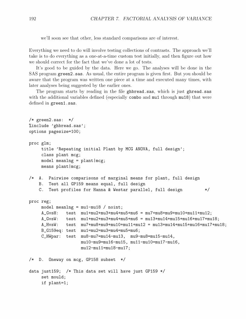
It’s good to be guided by the data. Here we go. The analyses will be done in theSAS program green2.sas. As usual, the entire program is given first. But you should beaware that the program was written one piece at a time and executed many times, withlater analyses being suggested by the earlier ones.
The program starts by reading in the file ghbread.sas, which is just ghread.sas
with the additional variables defined (especially combo and mu1 through mu18) that weredefined in green1.sas.
/* green2.sas: */
%include ’ghbread.sas’;
options pagesize=100;
proc glm;
title ’Repeating initial Plant by MCG ANOVA, full design’;
class plant mcg;
model meanlng = plant|mcg;
means plant|mcg;
/* A. Pairwise comparisons of marginal means for plant, full design
B. Test all GP159 means equal, full design
C. Test profiles for Hanna & Westar parallel, full design */
proc reg;
model meanlng = mu1-mu18 / noint;
A_GvsH: test mu1+mu2+mu3+mu4+mu5+mu6 = mu7+mu8+mu9+mu10+mu11+mu12;
A_GvsW: test mu1+mu2+mu3+mu4+mu5+mu6 = mu13+mu14+mu15+mu16+mu17+mu18;
A_HvsW: test mu7+mu8+mu9+mu10+mu11+mu12 = mu13+mu14+mu15+mu16+mu17+mu18;
B_G159eq: test mu1=mu2=mu3=mu4=mu5=mu6;
C_HWpar: test mu8-mu7=mu14-mu13, mu9-mu8=mu15-mu14,
mu10-mu9=mu16-mu15, mu11-mu10=mu17-mu16,
mu12-mu11=mu18-mu17;
/* D. Oneway on mcg, GP158 subset */
data just159; /* This data set will have just GP159 */
set mould;
if plant=1;

7.3. ANOTHER EXAMPLE: THE GREENHOUSE STUDY 193
proc glm data=just159;
title ’D. Oneway on mcg, GP158 subset’;
class mcg;
model meanlng = mcg;
/* E. Plant by MCG, Hanna-Westar subset */
data hanstar; /* This data set will have just Hanna and Westar */
set mould;
if plant ne 1;
proc glm data=hanstar;
title ’E. Plant by MCG, Hanna-Westar subset’;
class plant mcg;
model meanlng = plant|mcg;
/* F. Plant by MCG followup, Hanna-Westar subset
Interaction: Follow with all pairwise differences of
Westar minus Hanna differences
G. Differences within Hanna?
H. Differences within Westar? */
proc reg;
model meanlng = mu7-mu18 / noint;
F_inter: test mu13-mu7=mu14-mu8=mu15-mu9
= mu16-mu10=mu17-mu11=mu18-mu12;
F_1vs2: test mu13-mu7=mu14-mu8;
F_1vs3: test mu13-mu7=mu15-mu9;
F_1vs7: test mu13-mu7=mu16-mu10;
F_1vs8: test mu13-mu7=mu17-mu11;
F_1vs9: test mu13-mu7=mu18-mu12;
F_2vs3: test mu14-mu8=mu15-mu9;
F_2vs7: test mu14-mu8=mu16-mu10;
F_2vs8: test mu14-mu8=mu17-mu11;
F_2vs9: test mu14-mu8=mu18-mu12;
F_3vs7: test mu15-mu9=mu16-mu10;
F_3vs8: test mu15-mu9=mu17-mu11;
F_3vs9: test mu15-mu9=mu18-mu12;
F_7vs8: test mu16-mu10=mu17-mu11;
F_7vs9: test mu16-mu10=mu18-mu12;
F_8vs9: test mu17-mu11=mu18-mu12;
G_Hanaeq: test mu7=mu8=mu9=mu10=mu11=mu12;
H_Westeq: test mu13=mu14=mu15=mu16=mu17=mu18;
194 CHAPTER 7. FACTORIAL ANALYSIS OF VARIANCE
proc glm data=hanstar;
class combo;
model meanlng = combo;
lsmeans combo / pdiff adjust=scheffe;
proc iml;
title ’Table of Scheffe critical values for COLLECTIONS of contrasts’;
title2 ’Start with interaction’;
numdf = 5; /* Numerator degrees of freedom for initial test */
dendf = 60; /* Denominator degrees of freedom for initial test */
alpha = 0.05;
critval = finv(1-alpha,numdf,dendf);
zero = {0 0}; S_table = repeat(zero,numdf,1); /* Make empty matrix */
/* Label the columns */
namz = {"Number of Contrasts in followup test"
" Scheffe Critical Value"};
mattrib S_table colname=namz;
do i = 1 to numdf;
s_table(|i,1|) = i;
s_table(|i,2|) = numdf/i * critval;
end;
reset noname; /* Makes output look nicer in this case */
print "Initial test has" numdf " and " dendf "degrees of freedom."
"Using significance level alpha = " alpha;
print s_table;
proc iml;
title ’Table of Scheffe critical values for COLLECTIONS of contrasts’;
title2 ’Start with all means equal’;
numdf = 11; /* Numerator degrees of freedom for initial test */
dendf = 60; /* Denominator degrees of freedom for initial test */
alpha = 0.05;
critval = finv(1-alpha,numdf,dendf);
zero = {0 0}; S_table = repeat(zero,numdf,1); /* Make empty matrix */
/* Label the columns */
namz = {"Number of Contrasts in followup test"
" Scheffe Critical Value"};
mattrib S_table colname=namz;
do i = 1 to numdf;
s_table(|i,1|) = i;
s_table(|i,2|) = numdf/i * critval;
end;
reset noname; /* Makes output look nicer in this case */
print "Initial test has" numdf " and " dendf "degrees of freedom."
7.3. ANOTHER EXAMPLE: THE GREENHOUSE STUDY 195
"Using significance level alpha = " alpha;
print s_table;
proc reg data=hanstar;
title ’One more try at following up the interaction’;
model meanlng = mu7-mu18 / noint;
onemore: test mu8-mu7 = mu14-mu13;
After reading and defining the data with a %include statement, the program repeats theinitial three by six ANOVA from green1.sas. This is just for completeness. Then theSAS program performs tasks labelled A through H.
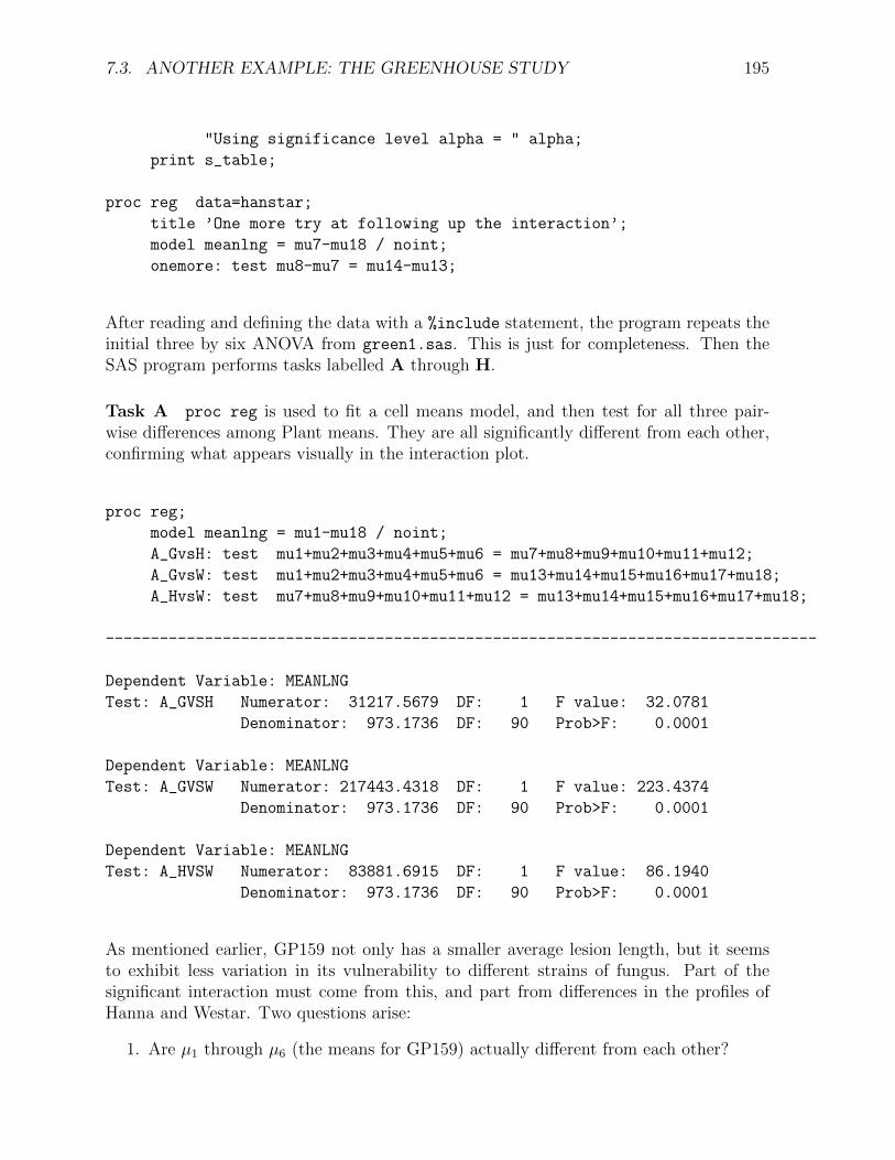
Task A proc reg is used to fit a cell means model, and then test for all three pair-wise differences among Plant means. They are all significantly different from each other,confirming what appears visually in the interaction plot.
proc reg;
model meanlng = mu1-mu18 / noint;
A_GvsH: test mu1+mu2+mu3+mu4+mu5+mu6 = mu7+mu8+mu9+mu10+mu11+mu12;
A_GvsW: test mu1+mu2+mu3+mu4+mu5+mu6 = mu13+mu14+mu15+mu16+mu17+mu18;
A_HvsW: test mu7+mu8+mu9+mu10+mu11+mu12 = mu13+mu14+mu15+mu16+mu17+mu18;
-------------------------------------------------------------------------------
Dependent Variable: MEANLNG
Test: A_GVSH Numerator: 31217.5679 DF: 1 F value: 32.0781
Denominator: 973.1736 DF: 90 Prob>F: 0.0001
Dependent Variable: MEANLNG
Test: A_GVSW Numerator: 217443.4318 DF: 1 F value: 223.4374
Denominator: 973.1736 DF: 90 Prob>F: 0.0001
Dependent Variable: MEANLNG
Test: A_HVSW Numerator: 83881.6915 DF: 1 F value: 86.1940
Denominator: 973.1736 DF: 90 Prob>F: 0.0001
As mentioned earlier, GP159 not only has a smaller average lesion length, but it seemsto exhibit less variation in its vulnerability to different strains of fungus. Part of thesignificant interaction must come from this, and part from differences in the profiles ofHanna and Westar. Two questions arise:
1. Are µ1 through µ6 (the means for GP159) actually different from each other?
196 CHAPTER 7. FACTORIAL ANALYSIS OF VARIANCE
2. Are the profiles for Hanna and Westar different?
There are two natural ways to address these questions. The naive way is to subset thedata — that is, do a one-way ANOVA to compare the 6 means for GP159, and a two-way(2 by 6) on the Hanna-Westar subset. In the latter analysis, the interaction of Plant byMCG would indicate whether the two profiles were different.
A more sophisticated approach is not to subset the data, but to recognize that bothquestions can be answered by testing collections of contrasts of the entire set of 18 means;it’s easy to do with the test statement of proc reg.
The advantage of the sophisticated approach is this. Remember that the model spec-ifies a conditional normal distribution of the dependent variable for each combination ofindependent variable values (in this case there are 18 combinations of independent variablevalues), and that each conditional distribution has the same variance. The test for, say,the equality of µ1 through µ6 would use only Y 1 through Y 6 (that is, just GP159 data) toestimate the 5 contrasts involved, but it would use all the data to estimate the commonerror variance. From both a commonsense viewpoint and the deepest possible theoreti-cal viewpoint, it’s better not to throw information away. This is why the sophisticatedapproach should be better.
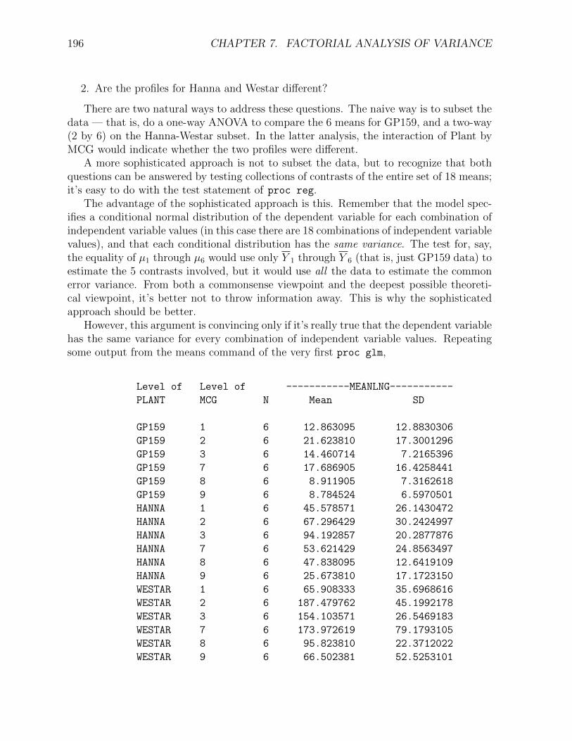
However, this argument is convincing only if it’s really true that the dependent variablehas the same variance for every combination of independent variable values. Repeatingsome output from the means command of the very first proc glm,
Level of Level of -----------MEANLNG-----------
PLANT MCG N Mean SD
GP159 1 6 12.863095 12.8830306
GP159 2 6 21.623810 17.3001296
GP159 3 6 14.460714 7.2165396
GP159 7 6 17.686905 16.4258441
GP159 8 6 8.911905 7.3162618
GP159 9 6 8.784524 6.5970501
HANNA 1 6 45.578571 26.1430472
HANNA 2 6 67.296429 30.2424997
HANNA 3 6 94.192857 20.2877876
HANNA 7 6 53.621429 24.8563497
HANNA 8 6 47.838095 12.6419109
HANNA 9 6 25.673810 17.1723150
WESTAR 1 6 65.908333 35.6968616
WESTAR 2 6 187.479762 45.1992178
WESTAR 3 6 154.103571 26.5469183
WESTAR 7 6 173.972619 79.1793105
WESTAR 8 6 95.823810 22.3712022
WESTAR 9 6 66.502381 52.5253101
7.3. ANOTHER EXAMPLE: THE GREENHOUSE STUDY 197
We see that the sample standard deviations for GP159 look quite a bit smaller on average.Without bothering to do a formal test, we have some reason to doubt the equal variancesassumption. It’s easy to see why GP159 would have less plant-to-plant variation in lesionlength. It’s so resistant to the fungus that there’s just not that much fungal growth,period. So there’s less opportunity for variation.
Note that the equal variances assumption is essentially just a mathematical conve-nience. Here, it’s clearly unrealistic. But what’s the consequence of violating it? It’swell known that the equal variance assumption can be safely violated if the cell samplesizes are equal and large. Well, here they’re equal, but n = 6 is not large. So this is notreassuring.
It’s not easy to say in general how the tests will be affected when the equal varianceassumption is violated, but for the two particular cases we’re interested in here (are theGP159 means equal and are the Hanna and Westar profiles parallel), we can figure it out.Formula 5.4 for the F -test (see page 130) says
F =(SSRF − SSRR)/r
MSEF.
The denominator (Mean Squared Error from the full model) is the estimated populationerror variance. That’s the variance that’s supposed to be the same for each conditionaldistribution. Since
MSE =
∑ni−1(Yi − Yi)2
n− p
and the predicted value Yi is always the cell mean, we can draw the following conclusions.Assume that the true variance is smaller for GP159.
1. When we test for equality of the GP159 means, using the Hanna-Westar data tohelp compute MSE will make the denominator of F bigger than it should be. So Fwill be smaller, and the test is too conservative. That is, it is less likely to detectdifferences that are really present.
2. When we test whether the Hanna and Westar profiles are parallel, use of the GP159data to help compute MSE will make the denominator of F smaller than it shouldbe – so F will be bigger, and the test will not be conservative enough. That is, thechance of significance if the effect is absent will be greater than 0.05. And a TypeI error rate above 0.05 is always to be avaoided if possible.
This makes me inclined to favour the ”naive” subsetting approach. Because the GP159means look so equal, and I want them to be equal, I’d like to give the test for differenceamong them the best possible chance. And because it looks like the profiles for Hanna andWestar are not parallel (and I want them to be non-parallel, because it’s more interestingif the effect of Fungus type depends on type of Plant), I want a more conservative test.
Another argument in favour of subsetting is based on botany rather than statistics.Hanna and Westar are commercial canola crop varieties, but while GP159 is definitely in
198 CHAPTER 7. FACTORIAL ANALYSIS OF VARIANCE
the canola family, it is more like a hardy weed than a food plant. It’s just a different kindof entity, and so analyzing its data separately makes a lot of sense.
You may wonder, if it’s so different, why was it included in the design in the firstplace? Well, taxonomically it’s quite similar to Hanna and Westar; really no one knewit would be such a vigorous monster in terms of resisting fungus. That’s why people doresearch – to find out things they didn’t already know.
Anyway, we’ll do the analysis both ways – both the seemingly naive way which isprobably better once you think about it, and the sophisticated way that uses the completeset of data for all analyses.
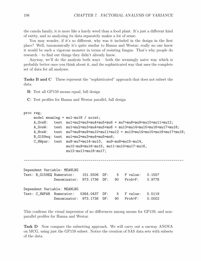
Tasks B and C These represent the “sophisticated” approach that does not subset thedata.
B: Test all GP159 means equal, full design
C: Test profiles for Hanna and Westar parallel, full design
proc reg;
model meanlng = mu1-mu18 / noint;
A_GvsH: test mu1+mu2+mu3+mu4+mu5+mu6 = mu7+mu8+mu9+mu10+mu11+mu12;
A_GvsW: test mu1+mu2+mu3+mu4+mu5+mu6 = mu13+mu14+mu15+mu16+mu17+mu18;
A_HvsW: test mu7+mu8+mu9+mu10+mu11+mu12 = mu13+mu14+mu15+mu16+mu17+mu18;
B_G159eq: test mu1=mu2=mu3=mu4=mu5=mu6;
C_HWpar: test mu8-mu7=mu14-mu13, mu9-mu8=mu15-mu14,
mu10-mu9=mu16-mu15, mu11-mu10=mu17-mu16,
mu12-mu11=mu18-mu17;
-------------------------------------------------------------------------------
Dependent Variable: MEANLNG
Test: B_G159EQ Numerator: 151.5506 DF: 5 F value: 0.1557
Denominator: 973.1736 DF: 90 Prob>F: 0.9778
Dependent Variable: MEANLNG
Test: C_HWPAR Numerator: 5364.0437 DF: 5 F value: 5.5119
Denominator: 973.1736 DF: 90 Prob>F: 0.0002
This confirms the visual impression of no differences among means for GP159, and non-parallel profiles for Hanna and Westar.
Task D Now compare the subsetting approach. We will carry out a oneway ANOVAon MCG, using just the GP159 subset. Notice the creation of SAS data sets with subsetsof the data.
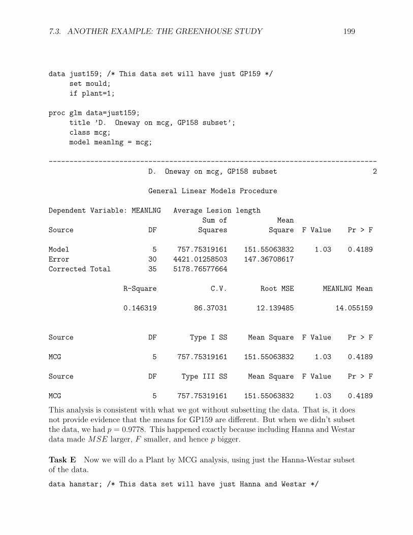
7.3. ANOTHER EXAMPLE: THE GREENHOUSE STUDY 199
data just159; /* This data set will have just GP159 */
set mould;
if plant=1;
proc glm data=just159;
title ’D. Oneway on mcg, GP158 subset’;
class mcg;
model meanlng = mcg;
-------------------------------------------------------------------------------
D. Oneway on mcg, GP158 subset 2
General Linear Models Procedure
Dependent Variable: MEANLNG Average Lesion length
Sum of Mean
Source DF Squares Square F Value Pr > F
Model 5 757.75319161 151.55063832 1.03 0.4189
Error 30 4421.01258503 147.36708617
Corrected Total 35 5178.76577664
R-Square C.V. Root MSE MEANLNG Mean
0.146319 86.37031 12.139485 14.055159
Source DF Type I SS Mean Square F Value Pr > F
MCG 5 757.75319161 151.55063832 1.03 0.4189
Source DF Type III SS Mean Square F Value Pr > F
MCG 5 757.75319161 151.55063832 1.03 0.4189
This analysis is consistent with what we got without subsetting the data. That is, it doesnot provide evidence that the means for GP159 are different. But when we didn’t subsetthe data, we had p = 0.9778. This happened exactly because including Hanna and Westardata made MSE larger, F smaller, and hence p bigger.
Task E Now we will do a Plant by MCG analysis, using just the Hanna-Westar subsetof the data.
data hanstar; /* This data set will have just Hanna and Westar */
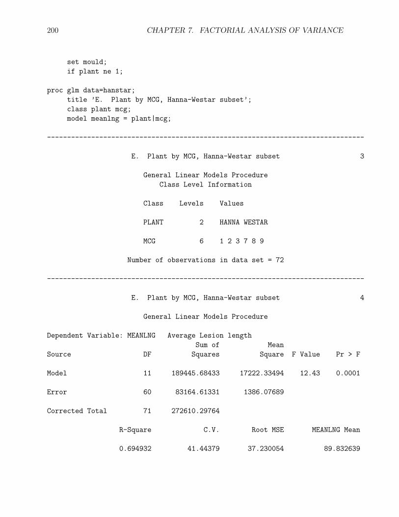
200 CHAPTER 7. FACTORIAL ANALYSIS OF VARIANCE
set mould;
if plant ne 1;
proc glm data=hanstar;
title ’E. Plant by MCG, Hanna-Westar subset’;
class plant mcg;
model meanlng = plant|mcg;
-------------------------------------------------------------------------------
E. Plant by MCG, Hanna-Westar subset 3
General Linear Models Procedure
Class Level Information
Class Levels Values
PLANT 2 HANNA WESTAR
MCG 6 1 2 3 7 8 9
Number of observations in data set = 72
-------------------------------------------------------------------------------
E. Plant by MCG, Hanna-Westar subset 4
General Linear Models Procedure
Dependent Variable: MEANLNG Average Lesion length
Sum of Mean
Source DF Squares Square F Value Pr > F
Model 11 189445.68433 17222.33494 12.43 0.0001
Error 60 83164.61331 1386.07689
Corrected Total 71 272610.29764
R-Square C.V. Root MSE MEANLNG Mean
0.694932 41.44379 37.230054 89.832639
7.3. ANOTHER EXAMPLE: THE GREENHOUSE STUDY 201
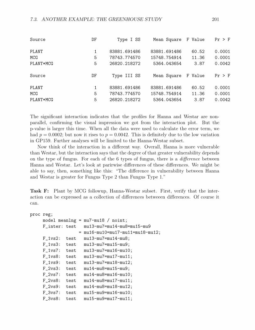
Source DF Type I SS Mean Square F Value Pr > F
PLANT 1 83881.691486 83881.691486 60.52 0.0001
MCG 5 78743.774570 15748.754914 11.36 0.0001
PLANT*MCG 5 26820.218272 5364.043654 3.87 0.0042
Source DF Type III SS Mean Square F Value Pr > F
PLANT 1 83881.691486 83881.691486 60.52 0.0001
MCG 5 78743.774570 15748.754914 11.36 0.0001
PLANT*MCG 5 26820.218272 5364.043654 3.87 0.0042
The significant interaction indicates that the profiles for Hanna and Westar are non-parallel, confirming the visual impression we got from the interaction plot. But thep-value is larger this time. When all the data were used to calculate the error term, wehad p = 0.0002; but now it rises to p = 0.0042. This is definitely due to the low variationin GP159. Further analyses will be limited to the Hanna-Westar subset.
Now think of the interaction in a different way. Overall, Hanna is more vulnerablethan Westar, but the interaction says that the degree of that greater vulnerability dependson the type of fungus. For each of the 6 types of fungus, there is a difference betweenHanna and Westar. Let’s look at parirwise differences of these differences. We might beable to say, then, something like this: “The difference in vulnerability between Hannaand Westar is greater for Fungus Type 2 than Fungus Type 1.”
Task F: Plant by MCG followup, Hanna-Westar subset. First, verify that the inter-action can be expressed as a collection of differences betweeen differences. Of course itcan.
proc reg;
model meanlng = mu7-mu18 / noint;
F_inter: test mu13-mu7=mu14-mu8=mu15-mu9
= mu16-mu10=mu17-mu11=mu18-mu12;
F_1vs2: test mu13-mu7=mu14-mu8;
F_1vs3: test mu13-mu7=mu15-mu9;
F_1vs7: test mu13-mu7=mu16-mu10;
F_1vs8: test mu13-mu7=mu17-mu11;
F_1vs9: test mu13-mu7=mu18-mu12;
F_2vs3: test mu14-mu8=mu15-mu9;
F_2vs7: test mu14-mu8=mu16-mu10;
F_2vs8: test mu14-mu8=mu17-mu11;
F_2vs9: test mu14-mu8=mu18-mu12;
F_3vs7: test mu15-mu9=mu16-mu10;
F_3vs8: test mu15-mu9=mu17-mu11;
202 CHAPTER 7. FACTORIAL ANALYSIS OF VARIANCE
F_3vs9: test mu15-mu9=mu18-mu12;
F_7vs8: test mu16-mu10=mu17-mu11;
F_7vs9: test mu16-mu10=mu18-mu12;
F_8vs9: test mu17-mu11=mu18-mu12;
-------------------------------------------------------------------------------
Dependent Variable: MEANLNG
Test: F_INTER Numerator: 5364.0437 DF: 5 F value: 3.8699
Denominator: 1386.077 DF: 60 Prob>F: 0.0042
Dependent Variable: MEANLNG
Test: F_1VS2 Numerator: 14956.1036 DF: 1 F value: 10.7902
Denominator: 1386.077 DF: 60 Prob>F: 0.0017
Dependent Variable: MEANLNG
Test: F_1VS3 Numerator: 2349.9777 DF: 1 F value: 1.6954
Denominator: 1386.077 DF: 60 Prob>F: 0.1979
Dependent Variable: MEANLNG
Test: F_1VS7 Numerator: 15006.4293 DF: 1 F value: 10.8265
Denominator: 1386.077 DF: 60 Prob>F: 0.0017
Dependent Variable: MEANLNG
Test: F_1VS8 Numerator: 1147.2776 DF: 1 F value: 0.8277
Denominator: 1386.077 DF: 60 Prob>F: 0.3666
Dependent Variable: MEANLNG
Test: F_1VS9 Numerator: 630.3018 DF: 1 F value: 0.4547
Denominator: 1386.077 DF: 60 Prob>F: 0.5027
Dependent Variable: MEANLNG
Test: F_2VS3 Numerator: 5449.1829 DF: 1 F value: 3.9314
Denominator: 1386.077 DF: 60 Prob>F: 0.0520
Dependent Variable: MEANLNG
Test: F_2VS7 Numerator: 0.0423 DF: 1 F value: 0.0000
Denominator: 1386.077 DF: 60 Prob>F: 0.9956
Dependent Variable: MEANLNG
Test: F_2VS8 Numerator: 7818.7443 DF: 1 F value: 5.6409
Denominator: 1386.077 DF: 60 Prob>F: 0.0208
Dependent Variable: MEANLNG
7.3. ANOTHER EXAMPLE: THE GREENHOUSE STUDY 203
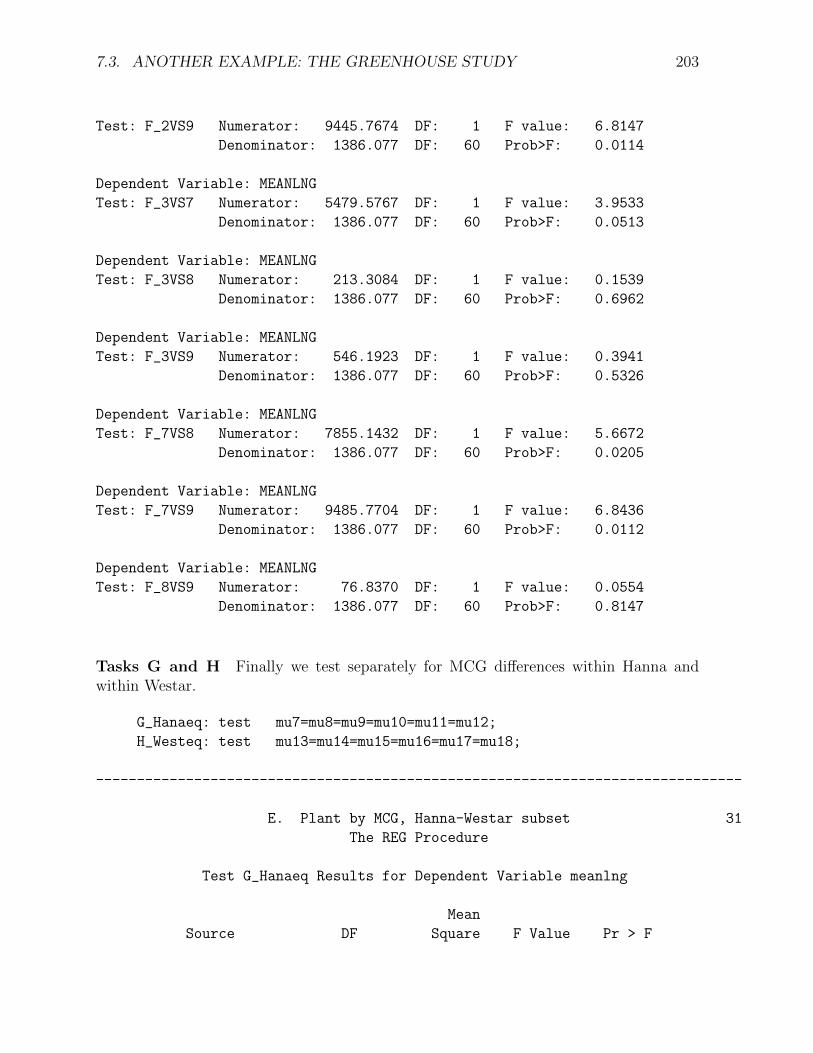
Test: F_2VS9 Numerator: 9445.7674 DF: 1 F value: 6.8147
Denominator: 1386.077 DF: 60 Prob>F: 0.0114
Dependent Variable: MEANLNG
Test: F_3VS7 Numerator: 5479.5767 DF: 1 F value: 3.9533
Denominator: 1386.077 DF: 60 Prob>F: 0.0513
Dependent Variable: MEANLNG
Test: F_3VS8 Numerator: 213.3084 DF: 1 F value: 0.1539
Denominator: 1386.077 DF: 60 Prob>F: 0.6962
Dependent Variable: MEANLNG
Test: F_3VS9 Numerator: 546.1923 DF: 1 F value: 0.3941
Denominator: 1386.077 DF: 60 Prob>F: 0.5326
Dependent Variable: MEANLNG
Test: F_7VS8 Numerator: 7855.1432 DF: 1 F value: 5.6672
Denominator: 1386.077 DF: 60 Prob>F: 0.0205
Dependent Variable: MEANLNG
Test: F_7VS9 Numerator: 9485.7704 DF: 1 F value: 6.8436
Denominator: 1386.077 DF: 60 Prob>F: 0.0112
Dependent Variable: MEANLNG
Test: F_8VS9 Numerator: 76.8370 DF: 1 F value: 0.0554
Denominator: 1386.077 DF: 60 Prob>F: 0.8147
Tasks G and H Finally we test separately for MCG differences within Hanna andwithin Westar.
G_Hanaeq: test mu7=mu8=mu9=mu10=mu11=mu12;
H_Westeq: test mu13=mu14=mu15=mu16=mu17=mu18;
-------------------------------------------------------------------------------
E. Plant by MCG, Hanna-Westar subset 31
The REG Procedure
Test G_Hanaeq Results for Dependent Variable meanlng
Mean
Source DF Square F Value Pr > F
204 CHAPTER 7. FACTORIAL ANALYSIS OF VARIANCE
Numerator 5 3223.58717 2.33 0.0536
Denominator 60 1386.07689
-------------------------------------------------------------------------------
Test H_Westeq Results for Dependent Variable meanlng
Mean
Source DF Square F Value Pr > F
Numerator 5 17889 12.91 <.0001
Denominator 60 1386.07689
There is evidence of differences in mean lesion length within Westar, but not Hanna. Itmakes sense to follow up with pairwise comparisons of the MCG means for just Westar,but first let’s review what we’ve done so far, limiting the discussion to just the Hanna-Westar subset of the data. We’ve tested
• Overall difference among the 12 means
• Main effect for PLANT
• Main effect for MCG
• PLANT*MCG interaction
• 15 pairwise comparisons of the Hanna-Westar difference, following up the interaction
• One comparison of the 6 means for Hanna
• One comparison of the 6 means for Westar
That’s 21 tests in all, and we really should do at least 15 more, testing for pairwisedifferences among the Westar means. Somehow, we should make this into a set of properpost-hoc tests, and correct for the fact that we’ve done a lot of them. But how? Tukeytests are only good for pairwise comparisons, and a Bonferroni correction is very ill-advised, since these tests were not all planned before seeing the data. This pretty muchleaves us with Scheffe or nothing.
Scheffe Tests Because some of the tests we’ve done are for more than one contrast at atime, the discussion of Scheffe tests for collections of contrasts in Section 3.4.5 (page 94)is relevant. But Section 3.4.5 is focused on the case where we are following up a significantdifference among all the treatment means. Here, the initial test may or may not be atest for equality of all the means. We might start somewhere else, like with a test for aninteraction or main effect. It’s a special case of Scheffe tests for regression (Section 5.10,page 133).
7.3. ANOTHER EXAMPLE: THE GREENHOUSE STUDY 205
Assume a multifactor design. Create a combination independent variable whose valuesare all combinations of factor levels. All the tests we do will be tests for collectionsconsisting of one or more contrasts of the cell means. Start with a statistically significantinitial test, an F -test for r contrasts. A Scheffe follow-up test will be a test for s contrasts,not necessarily a subset of the contrasts of the initial test. The follow-up test must obeythese rules:
• s < r
• If all r contrasts of the initial test are zero in the population, then all s contrasts ofthe follow-up test must be zero in the population. In other words, the null hypothesisof the follow-up test must be implied by the null hypothesis of the initial test. (Thefollow-up tests are proper follow-ups; see Section 3.4.6, page 96).
Next, compute the ordinary one-at-a-time F statistic for the follow-up test (it will haves and n − p degrees of freedom). Then, use the Scheffe critical value of Equation 5.8 onpage 133, which is repeated here for convenience:
fSch =r
sfcrit,
where fcrit is the usual critical value for the initial test. Then, considered as a Scheffefollow-up, the test is significant at the joint 0.05 level if the computed value of F for thecollection of contrasts is greater than fSch.
Actually, the formula given above is more general. It applies to testing linear combina-tions of regression coefficients in a multiple regression setting (see Section 5.10, page 133).The initial test is a test of r linear constraints on the regression coefficients, and the follow-up test is a test of s linear constraints, where s < r and the linear constraints of the initialtest imply the linear constraints of the follow-up test. This is very nice because it allows,for example, Scheffe follow-ups to a significant analysis of covariance.
Before applying Scheffe adjustments to the tests we have done on the greenhouse data,a few comments are in order.
• The term “linear constraints” may sound imposing, but a linear constraint is justa statement that some linear combination equals a constant. Almost always, theconstant is zero. So for example, saying that a contrast of cell means is equal to zerois the same as specifying a linear constraint on the betas of a multiple regressionmodel (for example, with cell means coding).
• If you’re testing 6 independent variables controlling for some other set of independentvariables, the null hypothesis says that 6 regression coefficients are equal to zero.That’s six linear constraints on the regression coefficients.
• In the initial one-way ANOVA setting (Section 3.4.3, page 89) where we were testingsingle contrasts of p cell means, the Scheffe adjusted criticl value was defined byfSch = (p − 1)fcrit. This was a special case of fSch = r
sfcrit. The initial test for
equality of p means involved p− 1 contrasts, so r = p− 1. The followup tests wereall for single contrasts, so s = 1.
206 CHAPTER 7. FACTORIAL ANALYSIS OF VARIANCE
• As in the case of testing single contrasts in a one-way design, it is impossible for afollowup to be significant if the initial test is not. And if the initial test is significant,there is always something to find in the family of Scheffe follow-ups.
• Suppose we have a follow-up test for s linear constraints, and it’s not significant.Then every Scheffe follow-up test whose null hypothesis is implied by those con-straints will also be non-significant. To use the metaphor of data fishing, onceyou’ve looked for fish in a particular region of the lake and determined that there’snothing there, further detailed exploration in that region is a waste of time.
The formula fSch = rsfcrit is very simple to apply. There are only two potential
complications, and they are related to one another.
• First, you have to know what significance test you are following up. For example,if your initial test is the test for equality of all cell means, then the test for a givenmain effect could be carried out as a Scheffe follow-up, and a pairwise comparison ofmarginal means would be another follow-up to the same initial test. Or, you couldstart with the test for the main effect. Then, the pairwise comparison of marginalmeans would be a follow-up to the one-at-a-time test for the main effect. You coulddo it either way, and the conclusions might differ. Where you start is a matter ofdata-analytic philosophy. But starting with the standard tests for main effects andinteractions is more traditional.
• The second potential complication is that you really have to be sure that the nullhypothesis of the initial test implies the null hypothesis of the follow-up test. Interms of proc reg syntax, it means that the test statement of the initial testimplies the test statements of all the follow-up tests. Sometimes this is easy tocheck, and sometimes it is tricky. To a large extent, how easy it is to check dependson what the initial test is.
– If the initial test is a test for all cell means being equal (a one-way ANOVAon the combination variable), then it’s easy, because if all the cell means areequal, then any possible contrast of the cell means equals zero. The proof isone line of High School algebra.
– Similarly, suppose we are using a regression model with an intercept, and theinitial test is for all the regression coefficients except β0 simultaneously. Thismeans that the null hypothesis of the initial test is H0 : β1 = . . . = βp−1 = 0,and therefore any linear combination of those quantities is zero. This meansthat you can test any subset of independent variables controlling for all theothers as a proper Scheffe follow-up to the first test SAS prints.
– If you’re following up tests for main effects, then the standard test for anycontrast of marginal means is a proper follow-up to the test for the main effect.
Beyond these principles, the logical connection between initial and follow-up tests reallyneeds to be checked on a case-by-case basis. Often, the initial test can be expressed
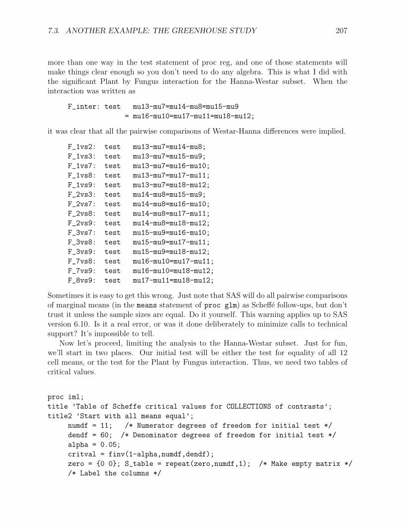
7.3. ANOTHER EXAMPLE: THE GREENHOUSE STUDY 207
more than one way in the test statement of proc reg, and one of those statements willmake things clear enough so you don’t need to do any algebra. This is what I did withthe significant Plant by Fungus interaction for the Hanna-Westar subset. When theinteraction was written as
F_inter: test mu13-mu7=mu14-mu8=mu15-mu9
= mu16-mu10=mu17-mu11=mu18-mu12;
it was clear that all the pairwise comparisons of Westar-Hanna differences were implied.
F_1vs2: test mu13-mu7=mu14-mu8;
F_1vs3: test mu13-mu7=mu15-mu9;
F_1vs7: test mu13-mu7=mu16-mu10;
F_1vs8: test mu13-mu7=mu17-mu11;
F_1vs9: test mu13-mu7=mu18-mu12;
F_2vs3: test mu14-mu8=mu15-mu9;
F_2vs7: test mu14-mu8=mu16-mu10;
F_2vs8: test mu14-mu8=mu17-mu11;
F_2vs9: test mu14-mu8=mu18-mu12;
F_3vs7: test mu15-mu9=mu16-mu10;
F_3vs8: test mu15-mu9=mu17-mu11;
F_3vs9: test mu15-mu9=mu18-mu12;
F_7vs8: test mu16-mu10=mu17-mu11;
F_7vs9: test mu16-mu10=mu18-mu12;
F_8vs9: test mu17-mu11=mu18-mu12;
Sometimes it is easy to get this wrong. Just note that SAS will do all pairwise comparisonsof marginal means (in the means statement of proc glm) as Scheffe follow-ups, but don’ttrust it unless the sample sizes are equal. Do it yourself. This warning applies up to SASversion 6.10. Is it a real error, or was it done deliberately to minimize calls to technicalsupport? It’s impossible to tell.
Now let’s proceed, limiting the analysis to the Hanna-Westar subset. Just for fun,we’ll start in two places. Our initial test will be either the test for equality of all 12cell means, or the test for the Plant by Fungus interaction. Thus, we need two tables ofcritical values.
proc iml;
title ’Table of Scheffe critical values for COLLECTIONS of contrasts’;
title2 ’Start with all means equal’;
numdf = 11; /* Numerator degrees of freedom for initial test */
dendf = 60; /* Denominator degrees of freedom for initial test */
alpha = 0.05;
critval = finv(1-alpha,numdf,dendf);
zero = {0 0}; S_table = repeat(zero,numdf,1); /* Make empty matrix */
/* Label the columns */
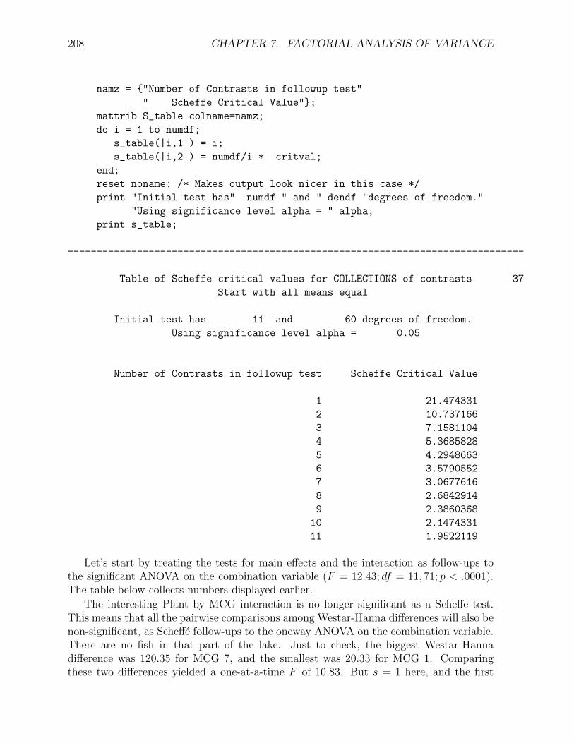
208 CHAPTER 7. FACTORIAL ANALYSIS OF VARIANCE
namz = {"Number of Contrasts in followup test"
" Scheffe Critical Value"};
mattrib S_table colname=namz;
do i = 1 to numdf;
s_table(|i,1|) = i;
s_table(|i,2|) = numdf/i * critval;
end;
reset noname; /* Makes output look nicer in this case */
print "Initial test has" numdf " and " dendf "degrees of freedom."
"Using significance level alpha = " alpha;
print s_table;
-------------------------------------------------------------------------------
Table of Scheffe critical values for COLLECTIONS of contrasts 37
Start with all means equal
Initial test has 11 and 60 degrees of freedom.
Using significance level alpha = 0.05
Number of Contrasts in followup test Scheffe Critical Value
1 21.474331
2 10.737166
3 7.1581104
4 5.3685828
5 4.2948663
6 3.5790552
7 3.0677616
8 2.6842914
9 2.3860368
10 2.1474331
11 1.9522119
Let’s start by treating the tests for main effects and the interaction as follow-ups tothe significant ANOVA on the combination variable (F = 12.43; df = 11, 71; p < .0001).The table below collects numbers displayed earlier.
The interesting Plant by MCG interaction is no longer significant as a Scheffe test.This means that all the pairwise comparisons among Westar-Hanna differences will also benon-significant, as Scheffe follow-ups to the oneway ANOVA on the combination variable.There are no fish in that part of the lake. Just to check, the biggest Westar-Hannadifference was 120.35 for MCG 7, and the smallest was 20.33 for MCG 1. Comparingthese two differences yielded a one-at-a-time F of 10.83. But s = 1 here, and the first
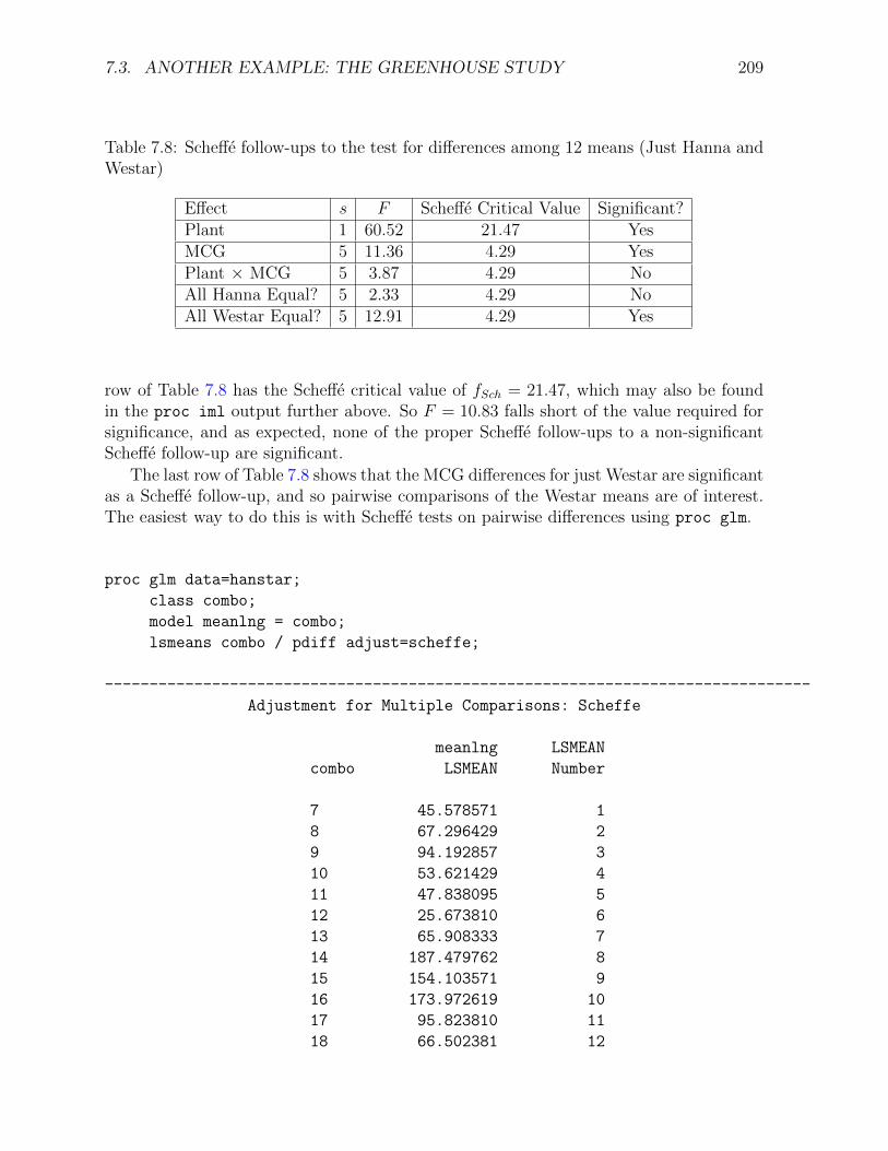
7.3. ANOTHER EXAMPLE: THE GREENHOUSE STUDY 209
Table 7.8: Scheffe follow-ups to the test for differences among 12 means (Just Hanna andWestar)
Effect s F Scheffe Critical Value Significant?Plant 1 60.52 21.47 YesMCG 5 11.36 4.29 YesPlant × MCG 5 3.87 4.29 NoAll Hanna Equal? 5 2.33 4.29 NoAll Westar Equal? 5 12.91 4.29 Yes
row of Table 7.8 has the Scheffe critical value of fSch = 21.47, which may also be foundin the proc iml output further above. So F = 10.83 falls short of the value required forsignificance, and as expected, none of the proper Scheffe follow-ups to a non-significantScheffe follow-up are significant.
The last row of Table 7.8 shows that the MCG differences for just Westar are significantas a Scheffe follow-up, and so pairwise comparisons of the Westar means are of interest.The easiest way to do this is with Scheffe tests on pairwise differences using proc glm.
proc glm data=hanstar;
class combo;
model meanlng = combo;
lsmeans combo / pdiff adjust=scheffe;
-------------------------------------------------------------------------------
Adjustment for Multiple Comparisons: Scheffe
meanlng LSMEAN
combo LSMEAN Number
7 45.578571 1
8 67.296429 2
9 94.192857 3
10 53.621429 4
11 47.838095 5
12 25.673810 6
13 65.908333 7
14 187.479762 8
15 154.103571 9
16 173.972619 10
17 95.823810 11
18 66.502381 12
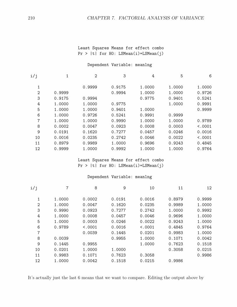
210 CHAPTER 7. FACTORIAL ANALYSIS OF VARIANCE
Least Squares Means for effect combo
Pr > |t| for H0: LSMean(i)=LSMean(j)
Dependent Variable: meanlng
i/j 1 2 3 4 5 6
1 0.9999 0.9175 1.0000 1.0000 1.0000
2 0.9999 0.9994 1.0000 1.0000 0.9726
3 0.9175 0.9994 0.9775 0.9401 0.5241
4 1.0000 1.0000 0.9775 1.0000 0.9991
5 1.0000 1.0000 0.9401 1.0000 0.9999
6 1.0000 0.9726 0.5241 0.9991 0.9999
7 1.0000 1.0000 0.9990 1.0000 1.0000 0.9789
8 0.0002 0.0047 0.0923 0.0008 0.0003 <.0001
9 0.0191 0.1620 0.7277 0.0457 0.0246 0.0016
10 0.0016 0.0235 0.2742 0.0046 0.0022 <.0001
11 0.8979 0.9989 1.0000 0.9696 0.9243 0.4845
12 0.9999 1.0000 0.9992 1.0000 1.0000 0.9764
Least Squares Means for effect combo
Pr > |t| for H0: LSMean(i)=LSMean(j)
Dependent Variable: meanlng
i/j 7 8 9 10 11 12
1 1.0000 0.0002 0.0191 0.0016 0.8979 0.9999
2 1.0000 0.0047 0.1620 0.0235 0.9989 1.0000
3 0.9990 0.0923 0.7277 0.2742 1.0000 0.9992
4 1.0000 0.0008 0.0457 0.0046 0.9696 1.0000
5 1.0000 0.0003 0.0246 0.0022 0.9243 1.0000
6 0.9789 <.0001 0.0016 <.0001 0.4845 0.9764
7 0.0039 0.1445 0.0201 0.9983 1.0000
8 0.0039 0.9955 1.0000 0.1071 0.0042
9 0.1445 0.9955 1.0000 0.7623 0.1518
10 0.0201 1.0000 1.0000 0.3058 0.0215
11 0.9983 0.1071 0.7623 0.3058 0.9986
12 1.0000 0.0042 0.1518 0.0215 0.9986
It’s actually just the last 6 means that we want to compare. Editing the output above by
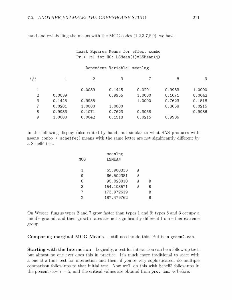
7.3. ANOTHER EXAMPLE: THE GREENHOUSE STUDY 211
hand and re-labelling the means with the MCG codes (1,2,3,7,8,9), we have
Least Squares Means for effect combo
Pr > |t| for H0: LSMean(i)=LSMean(j)
Dependent Variable: meanlng
i/j 1 2 3 7 8 9
1 0.0039 0.1445 0.0201 0.9983 1.0000
2 0.0039 0.9955 1.0000 0.1071 0.0042
3 0.1445 0.9955 1.0000 0.7623 0.1518
7 0.0201 1.0000 1.0000 0.3058 0.0215
8 0.9983 0.1071 0.7623 0.3058 0.9986
9 1.0000 0.0042 0.1518 0.0215 0.9986
In the following display (also edited by hand, but similar to what SAS produces withmeans combo / scheffe;) means with the same letter are not significantly different bya Scheffe test.
meanlng
MCG LSMEAN
1 65.908333 A
9 66.502381 A
8 95.823810 A B
3 154.103571 A B
7 173.972619 B
2 187.479762 B
On Westar, fungus types 2 and 7 grow faster than types 1 and 9; types 8 and 3 occupy amiddle ground, and their growth rates are not significantly different from either extremegroup.
Comparing marginal MCG Means I still need to do this. Put it in green2.sas.
Starting with the Interaction Logically, a test for interaction can be a follow-up test,but almost no one ever does this in practice. It’s much more traditional to start witha one-at-a-time test for interaction and then, if you’re very sophisticated, do multiplecomparison follow-ups to that initial test. Now we’ll do this with Scheffe follow-ups Inthe present case r = 5, and the critical values are obtaind from proc iml as before:
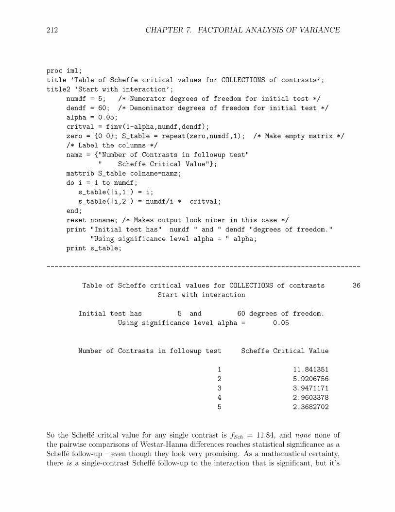
212 CHAPTER 7. FACTORIAL ANALYSIS OF VARIANCE
proc iml;
title ’Table of Scheffe critical values for COLLECTIONS of contrasts’;
title2 ’Start with interaction’;
numdf = 5; /* Numerator degrees of freedom for initial test */
dendf = 60; /* Denominator degrees of freedom for initial test */
alpha = 0.05;
critval = finv(1-alpha,numdf,dendf);
zero = {0 0}; S_table = repeat(zero,numdf,1); /* Make empty matrix */
/* Label the columns */
namz = {"Number of Contrasts in followup test"
" Scheffe Critical Value"};
mattrib S_table colname=namz;
do i = 1 to numdf;
s_table(|i,1|) = i;
s_table(|i,2|) = numdf/i * critval;
end;
reset noname; /* Makes output look nicer in this case */
print "Initial test has" numdf " and " dendf "degrees of freedom."
"Using significance level alpha = " alpha;
print s_table;
-------------------------------------------------------------------------------
Table of Scheffe critical values for COLLECTIONS of contrasts 36
Start with interaction
Initial test has 5 and 60 degrees of freedom.
Using significance level alpha = 0.05
Number of Contrasts in followup test Scheffe Critical Value
1 11.841351
2 5.9206756
3 3.9471171
4 2.9603378
5 2.3682702
So the Scheffe critcal value for any single contrast is fSch = 11.84, and none none ofthe pairwise comparisons of Westar-Hanna differences reaches statistical significance as aScheffe follow-up – even though they look very promising. As a mathematical certainty,there is a single-contrast Scheffe follow-up to the interaction that is significant, but it’s
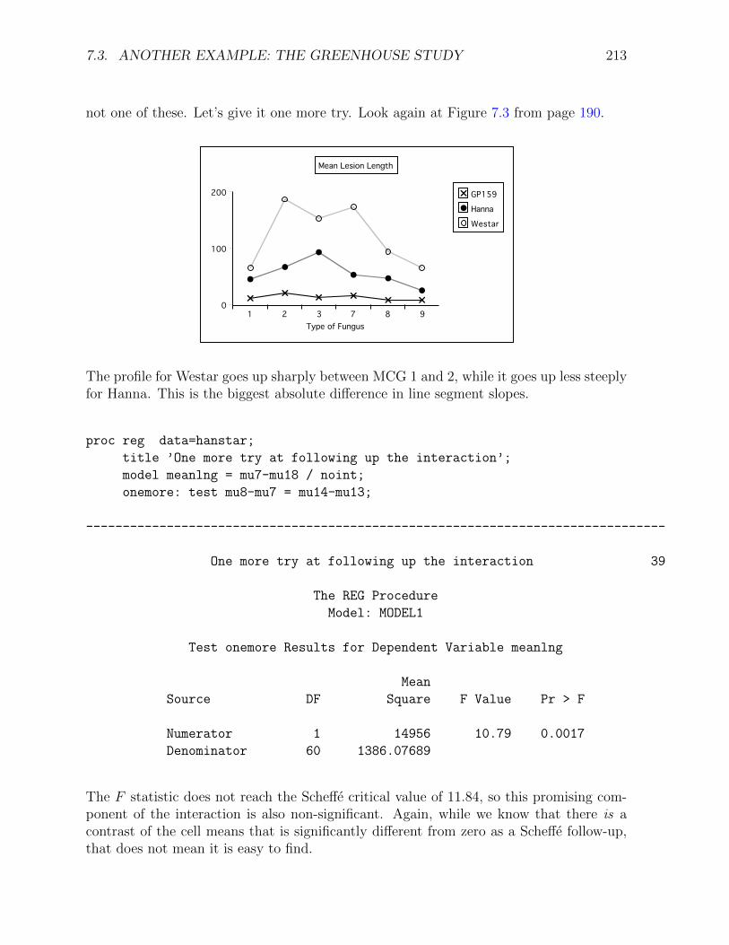
7.3. ANOTHER EXAMPLE: THE GREENHOUSE STUDY 213
not one of these. Let’s give it one more try. Look again at Figure 7.3 from page 190.
Chapter 7, Page 52
Denominator: 973.1736 DF: 90 Prob>F: 0.0001
Dependent Variable: MEANLNG
Test: FUNGUS Numerator: 11748.0529 DF: 5 F value: 12.0719
Denominator: 973.1736 DF: 90 Prob>F: 0.0001
Dependent Variable: MEANLNG
Test: P_BY_F Numerator: 4758.1481 DF: 10 F value: 4.8893
Denominator: 973.1736 DF: 90 Prob>F: 0.0001
Okay, now we know how to do anything. Finally, it is time to graph the interaction, and find out what these
results mean!
200
100
0
Type of Fungus1 2 3 7 8 9
Mean Lesion Length
GP159
Hanna
Westar
The profile for Westar goes up sharply between MCG 1 and 2, while it goes up less steeplyfor Hanna. This is the biggest absolute difference in line segment slopes.
proc reg data=hanstar;
title ’One more try at following up the interaction’;
model meanlng = mu7-mu18 / noint;
onemore: test mu8-mu7 = mu14-mu13;
-------------------------------------------------------------------------------
One more try at following up the interaction 39
The REG Procedure
Model: MODEL1
Test onemore Results for Dependent Variable meanlng
Mean
Source DF Square F Value Pr > F
Numerator 1 14956 10.79 0.0017
Denominator 60 1386.07689
The F statistic does not reach the Scheffe critical value of 11.84, so this promising com-ponent of the interaction is also non-significant. Again, while we know that there is acontrast of the cell means that is significantly different from zero as a Scheffe follow-up,that does not mean it is easy to find.