Chapter 7 · 85 Ganesh Sriram (ed.), Plant Metabolism: Methods and Protocols , Methods in Molecular Biology, vol. 1083, ... Jamey oung , Y

85

Ganesh Sriram (ed.), Plant Metabolism: Methods and Protocols, Methods in Molecular Biology, vol. 1083, DOI 10.1007/978-1-62703-661-0_7, © Springer Science+Business Media New York 2014

Chapter 7

Isotopomer Measurement Techniques in Metabolic Flux Analysis II: Mass Spectrometry

Jamey D. Young , Douglas K. Allen , and John A. Morgan

Abstract

Mass spectrometry (MS) offers a sensitive, reliable, and highly accurate method for measurement of isotopic labeling, which is required for generating comprehensive fl ux maps using metabolic fl ux analysis (MFA). We present protocols for assessing isotope labeling in a wide range of biochemical species, includ-ing proteinogenic amino acids, free organic and amino acids, sugar phosphates, lipids, starch-glucose, and RNA-ribose. We describe the steps of sample preparation, MS analysis, and data handling required to obtain high-quality isotope labeling measurements that are applicable to MFA. By selecting target analytes that maximize identifi ability of the key fl uxes of interest, MS measurements of isotope labeling can provide a powerful platform for assessing metabolic fl uxes in complex biochemical networks.

Key words Mass spectrometry , Metabolic fl ux analysis , Isotopomer , Proteinogenic amino acids , Sugar phosphates , Lipids , Starch , RNA , Ribose , GC-MS , LC-MS/MS

1 Introduction

The ability to quantitatively map intracellular fl uxes using meta-bolic fl ux analysis (MFA) is critical for identifying pathway bottle-necks and elucidating network regulation in biological systems, especially those that have been engineered to alter their native metabolic capacities [ 1 ]. MFA experiments involve feeding isoto-pically labeled substrates to cells, tissues, or whole organisms and subsequently measuring the patterns of isotope incorporation that occur in intracellular metabolites or secreted products. Both mass spectrometry (MS) and nuclear magnetic resonance (NMR) can be used to quantify the relative abundance of different “isoto-pomers” (i.e., isotope isomers) associated with each measured bio-molecule. MS provides a highly sensitive and accurate method for quantifying isotope incorporation, and has been increasingly used for MFA studies over the past decade. MS instruments are widely available and can be maintained and operated by individual labs, whereas NMR instruments are typically only available through

86

shared user facilities due to their high cost and operational com-plexity. This consideration along with the reduced sensitivity and longer analysis times of NMR has likely contributed to the increas-ing popularity of MS [ 2 ]. It should be noted, however, that datas-ets produced by MS and NMR often provide complementary information, and MFA strategies that combine both measurement technologies have been applied to maximize fl ux identifi ability in complex networks [ 3 , 4 ].

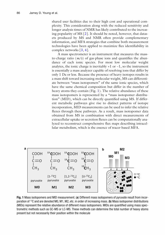
A mass spectrometer is an instrument that measures the mass-to- charge ratio ( m/z ) of gas-phase ions and quantifi es the abun-dance of each ionic species. For most low molecular weight analytes, the ionic charge is inevitably +1 or −1, so the instrument is essentially a mass analyzer capable of resolving ions that differ by only 1 Da or less. Because the presence of heavy isotopes results in a mass shift toward increasing molecular weight, MS can differenti-ate between “mass isotopomers” of the same ionic species, which have the same chemical composition but differ in the number of heavy atoms they contain (Fig. 1 ). The relative abundance of these mass isotopomers is represented by a “mass isotopomer distribu-tion” (MID), which can be directly quantifi ed using MS. If differ-ent metabolic pathways give rise to distinct patterns of isotope incorporation, MID measurements can be used to infer the relative fl uxes through these pathways. As a result, mass isotopomer data obtained from MS in combination with direct measurements of extracellular uptake or secretion fl uxes can be computationally ana-lyzed to reconstruct comprehensive fl ux maps describing intracel-lular metabolism, which is the essence of tracer- based MFA.

baM1

M2

M3M0

12C

13C

Fig. 1 Mass isotopomers and MID measurement. ( a ) Different mass isotopomers of pyruvate result from incor-poration of 13 C and are denoted M0, M1, M2, etc. in order of increasing mass. ( b ) Mass isotopomer distributions (MIDs) represent the relative abundance of different mass isotopomers. MIDs are quantifi ed using mass spec-trometric methods such as GC-MS or LC-MS. These methods can determine the total number of heavy atoms present but not necessarily their position within the molecule

Jamey D. Young et al.

87

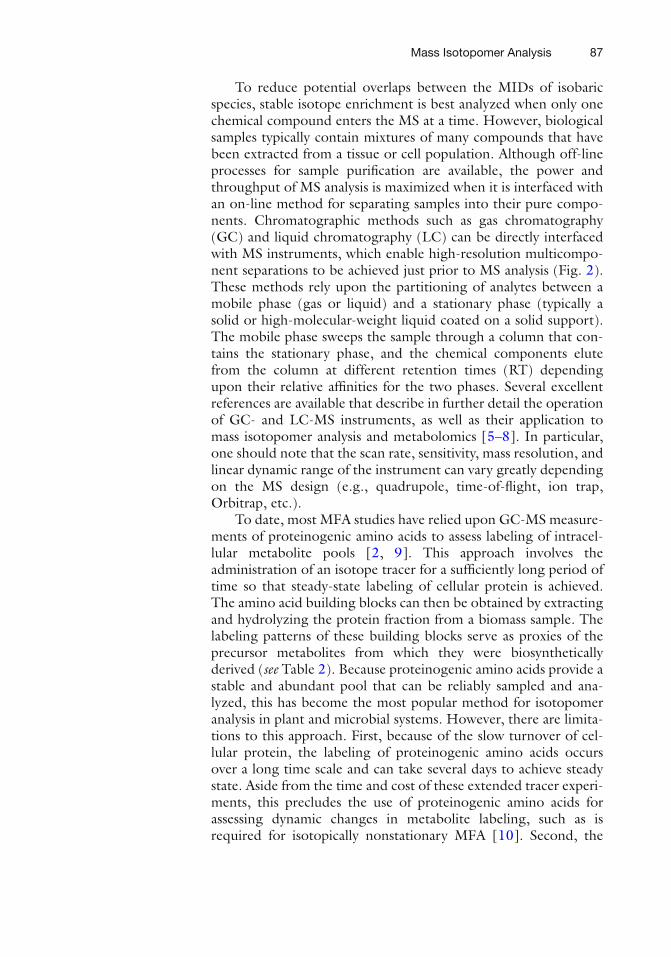
To reduce potential overlaps between the MIDs of isobaric species, stable isotope enrichment is best analyzed when only one chemical compound enters the MS at a time. However, biological samples typically contain mixtures of many compounds that have been extracted from a tissue or cell population. Although off-line processes for sample purifi cation are available, the power and throughput of MS analysis is maximized when it is interfaced with an on-line method for separating samples into their pure compo-nents. Chromatographic methods such as gas chromatography (GC) and liquid chromatography (LC) can be directly interfaced with MS instruments, which enable high-resolution multicompo-nent separations to be achieved just prior to MS analysis (Fig. 2 ). These methods rely upon the partitioning of analytes between a mobile phase (gas or liquid) and a stationary phase (typically a solid or high-molecular-weight liquid coated on a solid support). The mobile phase sweeps the sample through a column that con-tains the stationary phase, and the chemical components elute from the column at different retention times (RT) depending upon their relative affi nities for the two phases. Several excellent references are available that describe in further detail the operation of GC- and LC-MS instruments, as well as their application to mass isotopomer analysis and metabolomics [ 5 – 8 ]. In particular, one should note that the scan rate, sensitivity, mass resolution, and linear dynamic range of the instrument can vary greatly depending on the MS design (e.g., quadrupole, time-of-fl ight, ion trap, Orbitrap, etc.).

To date, most MFA studies have relied upon GC-MS measure-ments of proteinogenic amino acids to assess labeling of intracel-lular metabolite pools [ 2 , 9 ]. This approach involves the administration of an isotope tracer for a suffi ciently long period of time so that steady-state labeling of cellular protein is achieved. The amino acid building blocks can then be obtained by extracting and hydrolyzing the protein fraction from a biomass sample. The labeling patterns of these building blocks serve as proxies of the precursor metabolites from which they were biosynthetically derived ( see Table 2 ). Because proteinogenic amino acids provide a stable and abundant pool that can be reliably sampled and ana-lyzed, this has become the most popular method for isotopomer analysis in plant and microbial systems. However, there are limita-tions to this approach. First, because of the slow turnover of cel-lular protein, the labeling of proteinogenic amino acids occurs over a long time scale and can take several days to achieve steady state. Aside from the time and cost of these extended tracer experi-ments, this precludes the use of proteinogenic amino acids for assessing dynamic changes in metabolite labeling, such as is required for isotopically nonstationary MFA [ 10 ]. Second, the

Mass Isotopomer Analysis

88

m/z

0.0

0.2

0.4

0.6

0.8

1.0

370 371 372 373 374

m/z

rela

tive

inte

nsi

ty

0.0

0.2

0.4

0.6

0.8

1.0

173 174 175 176 177

m/z

rela

tive

inte

nsi

tyGas Chromatogram (GC)

(each peak is a different chemical compound)

Mass Isotopomer Distribution (MID)(of MS fragment ions at 173 and 370 m/z)

Mass spectrum (MS)(of GC peak at 11.6 min)

Fig. 2 Coupling GC with MS enables effi cient purifi cation and quantifi cation of mass isotopomers in complex biological samples. Chemical compounds are separated according to their retention times using gas chroma-tography. The mass spectrum of each compound is detected on-line as it elutes from the GC column. The MS data can be used to identify each compound based on the fragment ions it produces. MIDs of specifi c fragment ions can be extracted from the full MS scans and used to quantify isotope labeling


89

highly compartmented nature of plant cells places a higher burden on the experimentalist to obtain labeling information that can be used to resolve parallel fl uxes occurring simultaneously in separate organelles. This typically requires labeling data on carbohydrates, lipids, and other compounds that provide compartment-specifi c information complementary to that obtained from proteinogenic amino acids [ 11 ].

In light of the diverse array of MFA approaches and applica-tions that are now being considered, we have assembled a collec-tion of MS protocols applicable to several important classes of intracellular metabolites and macromolecules: proteinogenic amino acids, sugars from cellular RNA or starch, fatty acids from cellular lipid, and free intracellular metabolites (sugar phosphates, organic acids, amino acids, sugars). We do not attempt to provide protocols for extracting these compounds from plant tissues, as the appropriate methods can vary greatly depending on the tissue type. Typically, extraction of 20–100 mg of plant tissue is required to obtain suffi cient material for MS analysis, depending upon the tar-get compounds to be analyzed. For example, labeling in abundant pools such as protein and lipid can be readily determined by extracting 20 mg of plant tissue, whereas free metabolites may require 100 mg or more to achieve adequate signal-to-noise ratios. Furthermore, if free intracellular metabolites (e.g., sugar phos-phates or organic acids) are to be extracted from cells, care must be taken to rapidly quench all enzymatic activities immediately upon sampling so that the measured MIDs will provide an accurate refl ection of the in vivo labeling state [ 8 ].

Because GC-MS is a mature technology that has been used for qualitative and quantitative chemical analysis for over fi ve decades, we restrict our attention mainly to “tried-and-true” GC-MS methods. However, GC-MS is only applicable to analytes that are volatile or can be made so through chemical derivatiza-tion, and which furthermore do not thermally degrade at typical GC temperatures. For this reason, compounds such as sugar phosphates and CoA- containing molecules are often analyzed using LC-MS, which has the further advantage of not requiring any chemical derivatization steps. For example, the protocol pre-sented in Subheading 3.8 is based on an LC-MS method we have used for analysis of sugar phosphates in cyanobacterial extracts. It should also be noted that much recent progress has been made toward developing LC-MS methods for simultaneous analysis of metabolites from multiple chemical classes, and these “untar-geted” metabolomics approaches are becoming increasingly important in MFA studies [ 12 , 13 ]. However, the protocols pro-vided in this chapter will mainly describe “targeted” methods that have been used to analyze groups of similar compounds within a single chemical class.


90

2 Materials

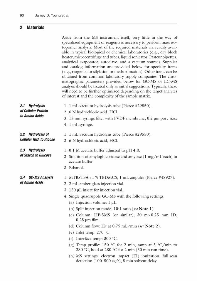
Aside from the MS instrument itself, very little in the way of specialized equipment or reagents is necessary to perform mass iso-topomer analysis. Most of the required materials are readily avail-able in typical biological or chemical laboratories (e.g., dry block heater, microcentrifuge and tubes, liquid sonicator, Pasteur pipettes, analytical evaporator, autoclave, and a vacuum source). Supplier and catalog information are provided below for specialty items (e.g., reagents for silylation or methoximation). Other items can be obtained from common laboratory supply companies. The chro-matographic parameters provided below for GC-MS or LC-MS analysis should be treated only as initial suggestions. Typically, these will need to be further optimized depending on the target analytes of interest and the complexity of the sample matrix.

1. 1 mL vacuum hydrolysis tube (Pierce #29550). 2. 6 N hydrochloric acid, HCl. 3. 13 mm syringe fi lter with PVDF membrane, 0.2 μm pore size. 4. 1 mL syringe.

1. 1 mL vacuum hydrolysis tube (Pierce #29550). 2. 6 N hydrochloric acid, HCl.

1. 0.1 M acetate buffer adjusted to pH 4.8. 2. Solution of amyloglucosidase and amylase (1 mg/mL each) in

acetate buffer. 3. Ethanol.

1. MTBSTFA +1 % TBDMCS, 1 mL ampules (Pierce #48927). 2. 2 mL amber glass injection vial. 3. 150 μL insert for injection vial. 4. Single quadrupole GC-MS with the following settings:

(a) Injection volume: 1 μL. (b) Split injection mode, 10:1 ratio ( see Note 1 ). (c) Column: HP-5MS (or similar), 30 m × 0.25 mm ID,

0.25 μm fi lm. (d) Column fl ow: He at 0.75 mL/min ( see Note 2 ). (e) Inlet temp: 270 °C. (f) Interface temp: 300 °C. (g) Temp profi le: 150 °C for 2 min, ramp at 5 °C/min to

280 °C, hold at 280 °C for 2 min (30 min run time). (h) MS settings: electron impact (EI) ionization, full-scan

detection (100–500 m/z ), 5 min solvent delay.

2.1 Hydrolysis of Cellular Protein to Amino Acids

2.2 Hydrolysis of Cellular RNA to Ribose

2.3 Hydrolysis of Starch to Glucose

2.4 GC-MS Analysis of Amino Acids


91

1. MOX reagent (Pierce #45950) or anhydrous pyridine ( see Note 3 ).

2. MTBSTFA +1 % TBDMCS, 1 mL ampules (Pierce #48927). 3. 2 mL amber glass injection vial. 4. 150 μL insert for injection vial. 5. Single quadrupole GC-MS with the following settings:

(a) Injection volume: 1 μL. (b) Purged splitless mode, set to activate at 1 min ( see Note 1 ). (c) Column: HP-5MS (or similar), 30 m × 0.25 mm ID, 0.25

μm fi lm. (d) Column fl ow: He at 1 mL/min ( see Note 2 ). (e) Inlet temp: 270 °C. (f) Interface temp: 300 °C. (g) Temp profi le: 80 °C for 2 min, ramp at 20 °C/min to

140 °C, ramp at 4 °C/min to 280 °C, hold at 280 °C for 5 min (45 min run time).

(h) MS settings: Scan mode (100–550), 5 min solvent delay.

1. 2 wt % hydroxylamine hydrochloride in pyridine solution (may be refrigerated up to 1 year).

2. Propionic anhydride. 3. Ethyl acetate. 4. 2 mL amber glass injection vial. 5. 150 μL insert for injection vial. 6. Single quadrupole GC-MS with the following settings:

(a) Injection volume: 1 μL. (b) Purged splitless mode, set to activate at 1 min ( see Note 1 ). (c) Column: HP-5MS (or similar), 30 m × 0.25 mm ID, 0.25

μm fi lm. (d) Column fl ow: He at 0.88 mL/min ( see Note 2 ). (e) Inlet temp: 250 °C. (f) Interface temp: 300 °C. (g) Temp profi le: 80 °C for 1 min, ramp at 20 °C/min to

280 °C, hold at 280 °C for 4 min (15 min run time). (h) MS settings: Scan mode (100–500), 5 min solvent delay.

1. 5 % (v/v) sulfuric acid dissolved in anhydrous methanol (fresh). 2. 0.2 % solution of butylated hydroxytoluene (BHT) in

methanol. 3. Toluene. 4. Hexane.

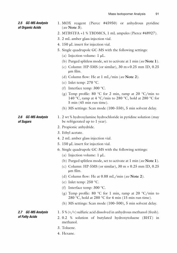
2.5 GC-MS Analysis of Organic Acids

2.6 GC-MS Analysis of Sugars

2.7 GC-MS Analysis of Fatty Acids


92

5. Screw-cap glass vial, with Tefl on-lined cap. 6. 2 mL amber glass injection vial. 7. Single quadrupole GC-MS with the following settings:

(a) Injection volume: 1 μL. (b) Purged splitless mode, set to activate at 1 min ( see Note 1 ). (c) Column: DB-23 (or similar), 30 m × 0.25 mm ID, 0.25 μm

fi lm ( see Note 4 ). (d) Column fl ow: He at 1 mL/min ( see Note 2 ). (e) Inlet temp: 250 °C. (f) Interface temp: 300 °C. (g) Temp profi le: 80 °C for 2 min, ramp at 20 °C/min to

140 °C, ramp at 10 °C/min to 240 °C, hold at 240 °C for 5 min (20 min run time).

(h) MS settings: Scan mode (50–500), 5 min solvent delay.

1. 13 mm syringe fi lter with PVDF membrane, 0.2 μm pore size. 2. 1 mL syringe. 3. 2 mL amber glass injection vial. 4. Eluent A: solution of 10 mM tributylamine +15 mM acetic

acid ( see Note 5 ). 5. Eluent B: HPLC-grade methanol. 6. Linear ion-trap triple quadrupole LC-MS/MS with the fol-

lowing settings: (a) Injection volume: 10 μL. (b) Column: Phenomenex Synergi Hydro-RP (or similar),

150 mm × 2.1 mm ID, 4 μm particle size. (c) Column fl ow: 0.3 mL/min. (d) Column temp: 25 °C. (e) Gradient profi le: 0 % B (0 min), 8 % B (8 min), 22 % B

(18 min), 40 % B (28 min), 60 % B (32 min), 90 % B (34 min), 90 % B (37 min), 0 % B (39 min), 0 % B (49 min).

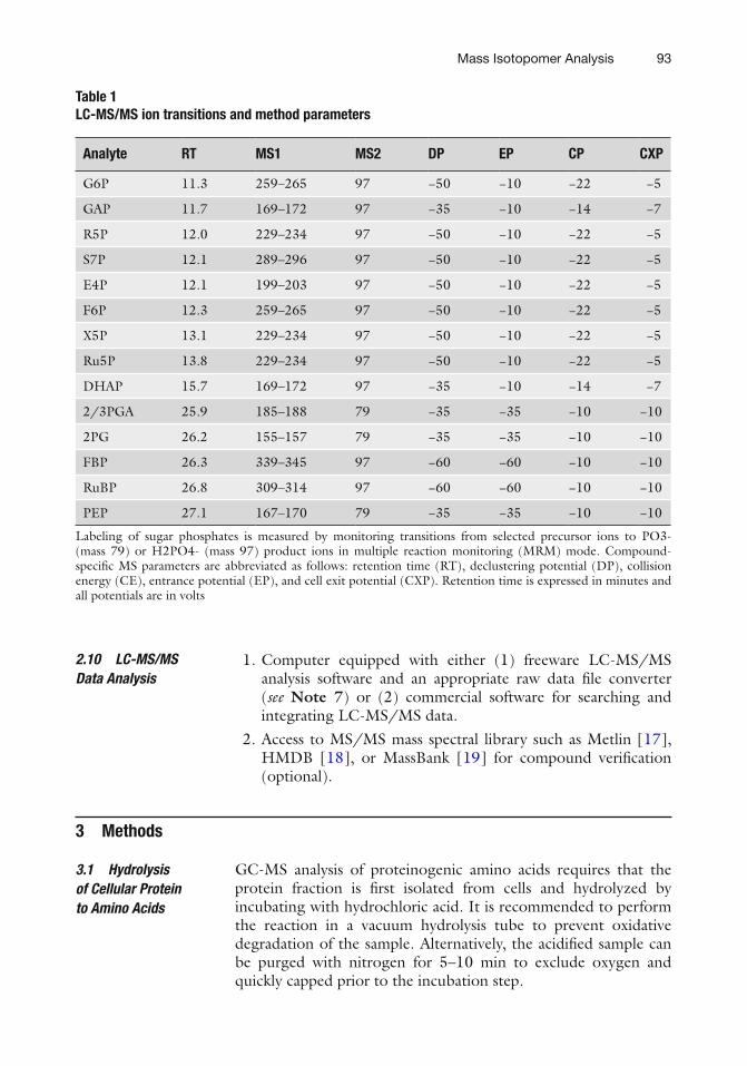
(f) MS settings: Negative-mode electrospray ionization (ESI), MRM mode ( see Table 1 and Note 6 ).

1. Computer equipped with AMDIS (freeware available at http://chemdata.nist.gov/mass-spc/amdis ), Wsearch32 (freeware available at http://www.wsearch.com.au/wsearch32/wsearch32.htm ), or commercial software for searching and integrating GC-MS data.

2. Mass spectral library such as the NIST/EPA/NIH Mass Spectral Database [ 14 ], Golm Metabolome Database [ 15 ], or FiehnLib [ 16 ] for compound identifi cation (optional).

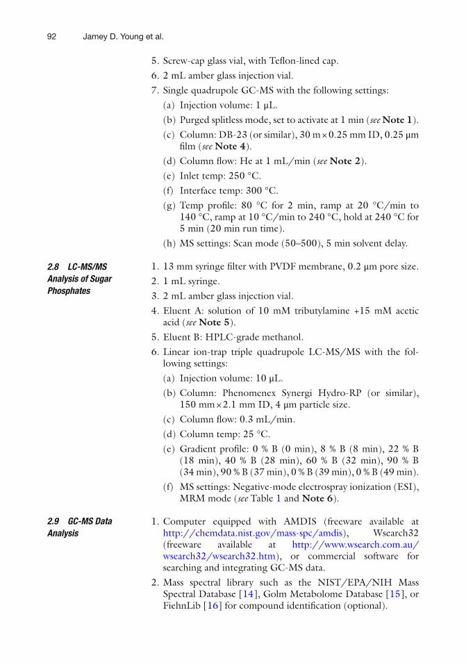
2.8 LC-MS/MS Analysis of Sugar Phosphates

2.9 GC-MS Data Analysis


http://chemdata.nist.gov/mass-spc/amdis

http://www.wsearch.com.au/wsearch32/wsearch32.htm

http://www.wsearch.com.au/wsearch32/wsearch32.htm

93

Table 1 LC-MS/MS ion transitions and method parameters

Analyte RT MS1 MS2 DP EP CP CXP

G6P 11.3 259–265 97 −50 −10 −22 −5

GAP 11.7 169–172 97 −35 −10 −14 −7

R5P 12.0 229–234 97 −50 −10 −22 −5

S7P 12.1 289–296 97 −50 −10 −22 −5

E4P 12.1 199–203 97 −50 −10 −22 −5

F6P 12.3 259–265 97 −50 −10 −22 −5

X5P 13.1 229–234 97 −50 −10 −22 −5

Ru5P 13.8 229–234 97 −50 −10 −22 −5

DHAP 15.7 169–172 97 −35 −10 −14 −7

2/3PGA 25.9 185–188 79 −35 −35 −10 −10

2PG 26.2 155–157 79 −35 −35 −10 −10

FBP 26.3 339–345 97 −60 −60 −10 −10

RuBP 26.8 309–314 97 −60 −60 −10 −10

PEP 27.1 167–170 79 −35 −35 −10 −10

Labeling of sugar phosphates is measured by monitoring transitions from selected precursor ions to PO3- (mass 79) or H2PO4- (mass 97) product ions in multiple reaction monitoring (MRM) mode. Compound-specifi c MS parameters are abbreviated as follows: retention time (RT), declustering potential (DP), collision energy (CE), entrance potential (EP), and cell exit potential (CXP). Retention time is expressed in minutes and all potentials are in volts

1. Computer equipped with either (1) freeware LC-MS/MS analysis software and an appropriate raw data fi le converter ( see Note 7 ) or (2) commercial software for searching and integrating LC-MS/MS data.

2. Access to MS/MS mass spectral library such as Metlin [ 17 ], HMDB [ 18 ], or MassBank [ 19 ] for compound verifi cation (optional).

3 Methods

GC-MS analysis of proteinogenic amino acids requires that the protein fraction is fi rst isolated from cells and hydrolyzed by incubating with hydrochloric acid. It is recommended to perform the reaction in a vacuum hydrolysis tube to prevent oxidative degradation of the sample. Alternatively, the acidifi ed sample can be purged with nitrogen for 5–10 min to exclude oxygen and quickly capped prior to the incubation step.

2.10 LC-MS/MS Data Analysis

3.1 Hydrolysis of Cellular Protein to Amino Acids


94

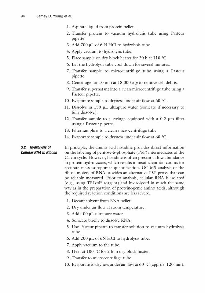
1. Aspirate liquid from protein pellet. 2. Transfer protein to vacuum hydrolysis tube using Pasteur

pipette. 3. Add 700 μL of 6 N HCl to hydrolysis tube. 4. Apply vacuum to hydrolysis tube. 5. Place sample on dry block heater for 20 h at 110 °C. 6. Let the hydrolysis tube cool down for several minutes. 7. Transfer sample to microcentrifuge tube using a Pasteur

pipette. 8. Centrifuge for 10 min at 18,000 × g to remove cell debris. 9. Transfer supernatant into a clean microcentrifuge tube using a

Pasteur pipette. 10. Evaporate sample to dryness under air fl ow at 60 °C. 11. Dissolve in 150 μL ultrapure water (sonicate if necessary to

fully dissolve). 12. Transfer sample to a syringe equipped with a 0.2 μm fi lter

using a Pasteur pipette. 13. Filter sample into a clean microcentrifuge tube. 14. Evaporate sample to dryness under air fl ow at 60 °C.

In principle, the amino acid histidine provides direct information on the labeling of pentose-5-phosphate (P5P) intermediates of the Calvin cycle. However, histidine is often present at low abundance in protein hydrolysates, which results in insuffi cient ion counts for accurate mass isotopomer quantifi cation. GC-MS analysis of the ribose moiety of RNA provides an alternative P5P proxy that can be reliably measured. Prior to analysis, cellular RNA is isolated (e.g., using TRIzol ® reagent) and hydrolyzed in much the same way as in the preparation of proteinogenic amino acids, although the required reaction conditions are less severe.

1. Decant solvent from RNA pellet. 2. Dry under air fl ow at room temperature. 3. Add 400 μL ultrapure water. 4. Sonicate briefl y to dissolve RNA. 5. Use Pasteur pipette to transfer solution to vacuum hydrolysis

tube. 6. Add 200 μL of 6N HCl to hydrolysis tube. 7. Apply vacuum to the tube. 8. Heat at 100 °C for 2 h in dry block heater. 9. Transfer to microcentrifuge tube. 10. Evaporate to dryness under air fl ow at 60 °C (approx. 120 min).

3.2 Hydrolysis of Cellular RNA to Ribose


95

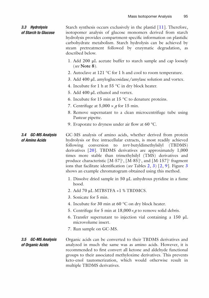
Starch synthesis occurs exclusively in the plastid [ 11 ]. Therefore, isotopomer analysis of glucose monomers derived from starch hydrolysis provides compartment-specifi c information on plastidic carbohydrate metabolism. Starch hydrolysis can be achieved by steam pretreatment followed by enzymatic degradation, as described below.

1. Add 200 μL acetate buffer to starch sample and cap loosely ( see Note 8 ).

2. Autoclave at 121 °C for 1 h and cool to room temperature. 3. Add 400 μL amyloglucosidase/amylase solution and vortex. 4. Incubate for 1 h at 55 °C in dry block heater. 5. Add 400 μL ethanol and vortex. 6. Incubate for 15 min at 15 °C to denature proteins. 7. Centrifuge at 5,000 × g for 15 min. 8. Remove supernatant to a clean microcentrifuge tube using

Pasteur pipette. 9. Evaporate to dryness under air fl ow at 60 °C.

GC-MS analysis of amino acids, whether derived from protein hydrolysis or free intracellular extracts, is most readily achieved following conversion to tert -butyldimethylsilyl (TBDMS) derivatives [ 20 ]. TBDMS derivatives are approximately 1,000 times more stable than trimethylsilyl (TMS) derivatives and produce characteristic [M-57] + , [M-85] + , and [M-157] + fragment ions that facilitate identifi cation ( see Tables 2 , 3 ) [ 2 , 9 ]. Figure 3 shows an example chromatogram obtained using this method.

1. Dissolve dried sample in 50 μL anhydrous pyridine in a fume hood.

2. Add 70 μL MTBSTFA +1 % TBDMCS. 3. Sonicate for 5 min. 4. Incubate for 30 min at 60 °C on dry block heater. 5. Centrifuge for 5 min at 18,000 × g to remove solid debris. 6. Transfer supernatant to injection vial containing a 150 μL

microvolume insert. 7. Run sample on GC-MS.

Organic acids can be converted to their TBDMS derivatives and analyzed in much the same was as amino acids. However, it is recommended to fi rst convert all ketone and aldehyde functional groups to their associated methyloxime derivatives. This prevents keto-enol tautomerization, which would otherwise result in multiple TBDMS derivatives.

3.3 Hydrolysis of Starch to Glucose

3.4 GC-MS Analysis of Amino Acids

3.5 GC-MS Analysis of Organic Acids


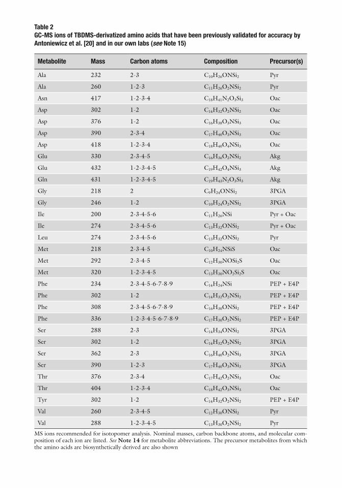
Table 2 GC-MS ions of TBDMS-derivatized amino acids that have been previously validated for accuracy by Antoniewicz et al. [20] and in our own labs (see Note 15)

Metabolite Mass Carbon atoms Composition Precursor(s)

Ala 232 2-3 C 10 H 26 ONSi 2 Pyr

Ala 260 1-2-3 C 11 H 26 O 2 NSi 2 Pyr

Asn 417 1-2-3-4 C 18 H 41 N 2 O 3 Si 3 Oac

Asp 302 1-2 C 14 H 32 O 2 NSi 2 Oac

Asp 376 1-2 C 16 H 38 O 3 NSi 3 Oac

Asp 390 2-3-4 C 17 H 40 O 3 NSi 3 Oac

Asp 418 1-2-3-4 C 18 H 40 O 4 NSi 3 Oac

Glu 330 2-3-4-5 C 16 H 36 O 2 NSi 2 Akg

Glu 432 1-2-3-4-5 C 19 H 42 O 4 NSi 3 Akg

Gln 431 1-2-3-4-5 C 19 H 43 N 2 O 3 Si 3 Akg

Gly 218 2 C 9 H 24 ONSi 2 3PGA

Gly 246 1-2 C 10 H 24 O 2 NSi 2 3PGA

Ile 200 2-3-4-5-6 C 11 H 26 NSi Pyr + Oac

Ile 274 2-3-4-5-6 C 13 H 32 ONSi 2 Pyr + Oac

Leu 274 2-3-4-5-6 C 13 H 32 ONSi 2 Pyr

Met 218 2-3-4-5 C 10 H 24 NSiS Oac

Met 292 2-3-4-5 C 12 H 30 NOSi 2 S Oac

Met 320 1-2-3-4-5 C 13 H 30 NO 2 Si 2 S Oac

Phe 234 2-3-4-5-6-7-8-9 C 14 H 24 NSi PEP + E4P

Phe 302 1-2 C 14 H 32 O 2 NSi 2 PEP + E4P

Phe 308 2-3-4-5-6-7-8-9 C 16 H 30 ONSi 2 PEP + E4P

Phe 336 1-2-3-4-5-6-7-8-9 C 17 H 30 O 2 NSi 2 PEP + E4P

Ser 288 2-3 C 14 H 34 ONSi 2 3PGA

Ser 302 1-2 C 14 H 32 O 2 NSi 2 3PGA

Ser 362 2-3 C 16 H 40 O 2 NSi 3 3PGA

Ser 390 1-2-3 C 17 H 40 O 3 NSi 3 3PGA

Thr 376 2-3-4 C 17 H 42 O 2 NSi 3 Oac

Thr 404 1-2-3-4 C 18 H 42 O 3 NSi 3 Oac

Tyr 302 1-2 C 14 H 32 O 2 NSi 2 PEP + E4P

Val 260 2-3-4-5 C 12 H 30 ONSi 2 Pyr

Val 288 1-2-3-4-5 C 13 H 30 O 2 NSi 2 Pyr

MS ions recommended for isotopomer analysis. Nominal masses, carbon backbone atoms, and molecular com-position of each ion are listed. See Note 14 for metabolite abbreviations. The precursor metabolites from which the amino acids are biosynthetically derived are also shown

97

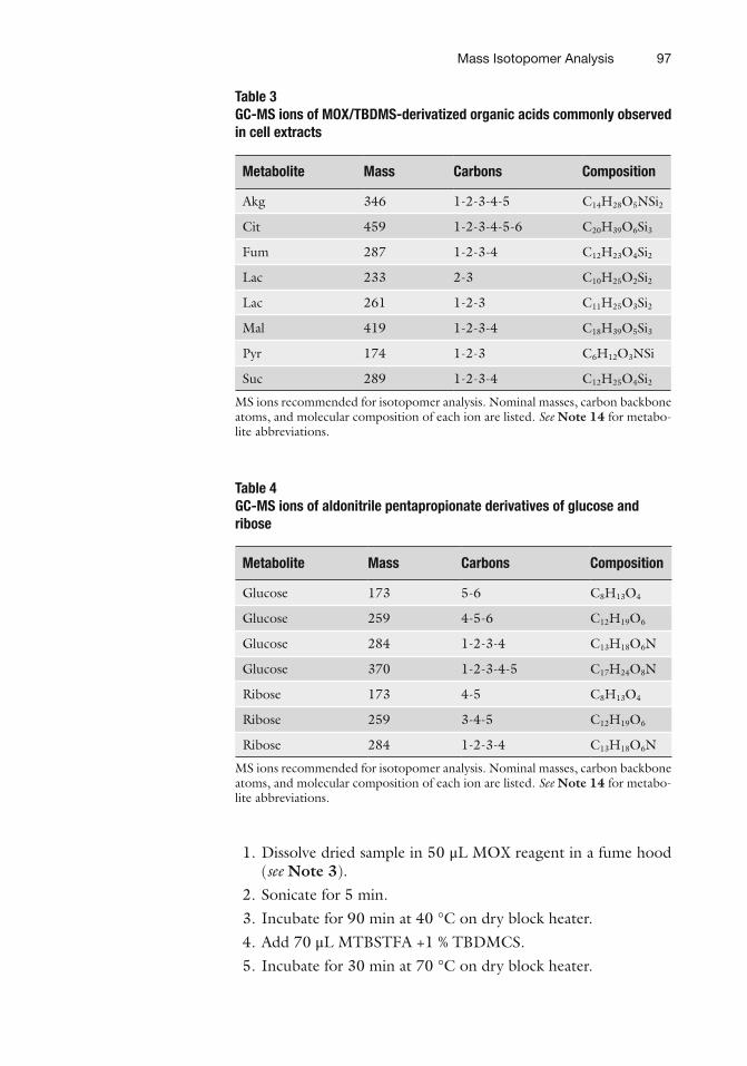
1. Dissolve dried sample in 50 μL MOX reagent in a fume hood ( see Note 3 ).

2. Sonicate for 5 min. 3. Incubate for 90 min at 40 °C on dry block heater. 4. Add 70 μL MTBSTFA +1 % TBDMCS. 5. Incubate for 30 min at 70 °C on dry block heater.

Table 3 GC-MS ions of MOX/TBDMS-derivatized organic acids commonly observed in cell extracts

Metabolite Mass Carbons Composition

Akg 346 1-2-3-4-5 C 14 H 28 O 5 NSi 2

Cit 459 1-2-3-4-5-6 C 20 H 39 O 6 Si 3

Fum 287 1-2-3-4 C 12 H 23 O 4 Si 2

Lac 233 2-3 C 10 H 25 O 2 Si 2

Lac 261 1-2-3 C 11 H 25 O 3 Si 2

Mal 419 1-2-3-4 C 18 H 39 O 5 Si 3

Pyr 174 1-2-3 C 6 H 12 O 3 NSi

Suc 289 1-2-3-4 C 12 H 25 O 4 Si 2

MS ions recommended for isotopomer analysis. Nominal masses, carbon backbone atoms, and molecular composition of each ion are listed. See Note 14 for metabo-lite abbreviations.

Table 4 GC-MS ions of aldonitrile pentapropionate derivatives of glucose and ribose


Glucose 173 5-6 C 8 H 13 O 4

Glucose 259 4-5-6 C 12 H 19 O 6

Glucose 284 1-2-3-4 C 13 H 18 O 6 N

Glucose 370 1-2-3-4-5 C 17 H 24 O 8 N

Ribose 173 4-5 C 8 H 13 O 4

Ribose 259 3-4-5 C 12 H 19 O 6

Ribose 284 1-2-3-4 C 13 H 18 O 6 N

MS ions recommended for isotopomer analysis. Nominal masses, carbon backbone atoms, and molecular composition of each ion are listed. See Note 14 for metabo-lite abbreviations.


98

6. Remove from heating block and incubate overnight at room temperature ( see Note 9 ).

7. Centrifuge for 5 min at 18,000 × g to remove solid debris. 8. Transfer liquid to injection vial containing a 150 μL microvol-

ume insert. 9. Run sample on GC-MS.

There is a wealth of information on carbohydrate metabolism that can be obtained from isotopomer analysis of sugars derived from RNA ( see Subheading 3.2 ), starch ( see Subheading 3.3 ), or free intracellular extracts. Furthermore, Allen et al. [ 11 ] have shown

3.6 GC-MS Analysis of Sugars

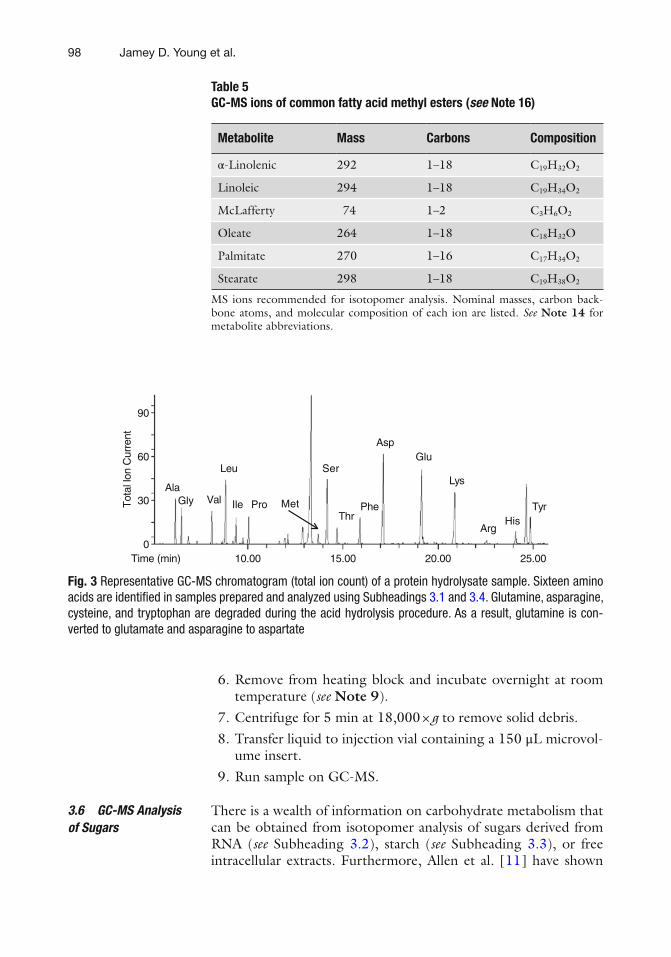
Table 5 GC-MS ions of common fatty acid methyl esters (see Note 16)


α-Linolenic 292 1–18 C 19 H 32 O 2

Linoleic 294 1–18 C 19 H 34 O 2

McLafferty 74 1–2 C 3 H 6 O 2

Oleate 264 1–18 C 18 H 32 O

Palmitate 270 1–16 C 17 H 34 O 2

Stearate 298 1–18 C 19 H 38 O 2

MS ions recommended for isotopomer analysis. Nominal masses, carbon back-bone atoms, and molecular composition of each ion are listed. See Note 14 for metabolite abbreviations.

Ala

Time (min)

Tot

al lo

n C

urre

nt

10.000

30

60

90

15.00 20.00 25.00

Gly Val

Leu

Ile Pro

Ser

Thr

AspGlu

Lys

Phe TyrMet

HisArg

Fig. 3 Representative GC-MS chromatogram (total ion count) of a protein hydrolysate sample. Sixteen amino acids are identifi ed in samples prepared and analyzed using Subheadings 3.1 and 3.4 . Glutamine, asparagine, cysteine, and tryptophan are degraded during the acid hydrolysis procedure. As a result, glutamine is con-verted to glutamate and asparagine to aspartate


99

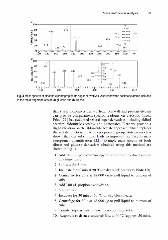
that sugar monomers derived from cell wall and protein glycans can provide compartment-specifi c readouts on cytosolic fl uxes. Price [ 21 ] has evaluated several sugar derivatives including alditol acetates, aldonitrile acetates, and peracetates. Here we provide a slight variation on the aldonitrile acetate approach, which replaces the acetate functionality with a propionate group. Antoniewicz has shown that this substitution leads to improved accuracy in mass isotopomer quantifi cation [ 22 ]. Example mass spectra of both ribose and glucose derivatives obtained using this method are shown in Fig. 4 .

1. Add 50 μL hydroxylamine/pyridine solution to dried sample in a fume hood.

2. Sonicate for 5 min. 3. Incubate for 60 min at 90 °C on dry block heater ( see Note 10 ). 4. Centrifuge for 30 s at 18,000 × g to pull liquid to bottom of

tube. 5. Add 100 μL propionic anhydride. 6. Sonicate for 5 min. 7. Incubate for 30 min at 60 °C on dry block heater. 8. Centrifuge for 30 s at 18,000 × g to pull liquid to bottom of

tube. 9. Transfer supernatant to new microcentrifuge tube. 10. Evaporate to dryness under air fl ow at 60 °C (approx. 30 min).

Fig. 4 Mass spectra of aldonitrile pentapropionate sugar derivatives. Insets show the backbone atoms included in the main fragment ions of ( a ) glucose and ( b ) ribose


100

11. Add 100 μL of ethyl acetate. 12. Sonicate for 5 min ( see Note 11 ). 13. Centrifuge for 10 min at 18,000 × g to remove solids. 14. Transfer supernatant to GC injection vial containing a 150 μL

insert. 15. Run sample on GC-MS.

Isotopomer analysis of fatty acids derived from cellular lipids provides compartment-specifi c information on the labeling of acetyl- CoA pools [ 11 ]. Typically, lipids are extracted and transesterifi ed to generate fatty acid methyl esters (FAMEs), which are subsequently analyzed by GC-MS [ 6 , 23 ]. Other derivatization protocols can be found in the literature including the formation of butylamides [ 11 ]. Here, we present a commonly used acid- catalyzed transmethylation approach that is straightforward to perform.

1. Add 2 mL 5 % sulfuric acid in methanol (v/v) to dried sample in glass vial.

2. Add 0.5 mL toluene. 3. Add 25 μL 0.2 % BHT in methanol. 4. Vortex and heat at 95 °C for 2 h. 5. Add 3 mL ultrapure water and shake to quench reaction. 6. Extract twice with 3 mL hexane, using a Pasteur pipette to

remove extracts. 7. Pool hexane extracts and dry under air fl ow at room

temperature. 8. Dissolve in 1 mL hexane and transfer to GC injection vial. 9. Run sample on GC-MS.

Although analysis of labeling in macromolecule components such as protein, starch, and lipid has dominated the MFA literature due to their high abundance in tissues, recent advances in MS technology have facilitated direct analysis of free intracellular metabolites. This approach enables quantifi cation of MIDs in sugar phosphate intermediates that participate directly in glycolysis and Calvin cycle reactions, providing comprehensive and dynamic information on fl ux through these important pathways. (However, for intermediates found in multiple subcellular compartments this will only provide the average labeling among the various intracellular pools.) The vast majority of sugar phosphate analysis has been performed using LC-MS/MS, which avoids degradation of these heat-labile analytes [ 24 ]. The LC-MS/MS conditions provided in

3.7 GC-MS Analysis of Total Fatty Acids

3.8 LC-MS/MS Analysis of Sugar Phosphates


101

Subheading 2.8 are based on the method of Luo et al. [ 13 ], which has been subsequently modifi ed and applied to analyze labeling in cyanobacteria extracts by Shastri [ 25 ].

1. Evaporate solvent from deproteinized cell extract. 2. Dissolve in 1 mL ultrapure water and fi lter to remove

particulates. 3. Transfer to LC injection vial. 4. Run sample on LC-MS/MS.

Analysis of GC-MS data requires (1) identifi cation of chromatographic peaks and fragment ions associated with target analytes of interest, (2) integration of ion chromatograms over time to quantify relative abundance of specifi c isotope peaks, and (3) assessment of measurement standard errors. In many cases, it is also desirable to “correct” the raw MIDs to account for the presence of naturally occurring stable isotopes. Corrected mass isotopomer data provides a more intuitive picture of the labeling that is attributable to the introduction of a tracer compound and is generally the preferred method for presenting data from an isotope labeling experiment. However, note that some MFA software will perform these corrections internally, and therefore it is only necessary to input the raw, uncorrected MIDs in this case.

1. Identify the chromatographic peaks associated with analytes of interest. Identifi cation of chromatographic peaks is based on both the retention time (RT) and the MS fi ngerprint of the peak. If targeted analysis of a relatively small number of com-pounds (for which pure standards are available) is to be per-formed, then it is not necessary to use a comprehensive library search. The retention time and main fragment ions can be determined by running pure standards of each compound under the relevant GC-MS conditions, and then the sample chromatograms can be manually searched using available soft-ware tools to locate the corresponding peaks. However, untar-geted analysis is facilitated by using a mass spectral library to automatically search the GC-MS dataset for uniquely identi-fi ed “hits”. Retention time locked libraries are now available that contain both RT and MS information, which can further improve search reliability [ 16 ].

2. Identify ions to be used for mass isotopomer analysis. Once the chromatographic peaks of interest have been identifi ed, it is necessary to select the ions that will be used for mass isoto-pomer analysis and to determine their molecular composition. The best candidates are highly abundant ions with masses greater than 150 Da, since these are less likely to be contaminated by interfering fragment ions of similar mass. Determining the

3.9 GC-MS Data Analysis


102

elemental composition of these ionic species is facilitated by references that list common fragmentation patterns and molec-ular rearrangements obtained for particular classes of com-pounds and derivatization groups (e.g., see Kitson et al. [ 6 ]). Tables 2–5 lists several important fragment ions that are obtained using the methods described in this chapter, many of which have been utilized in previous MFA studies.

3. Integrate mass isotopomer peaks. In order to maximize the accu-racy of mass isotopomer data, it is necessary to integrate each ion chromatogram over its full peak width. This involves inte-grating all single ion traces over all scans of the peak, including masses up to 3 Da heavier than the fully labeled fragment ion ( see Note 12 ). For example, to quantify the MID of a fragment with monoisotopic mass 200 m/z and up to three labeled car-bons, extract and independently integrate the ion traces of 200, 201, 202,…, 206. Normalize the integrated areas such that the sum of all mass isotopomers for a given fragment ion is 1 (i.e., 100 mol%).

4. Correct MIDs for natural isotope abundance (optional). There has been much confusion in the literature over how to properly correct mass isotopomer data for the presence of naturally occurring isotopes. Most errors have resulted from improper handling of the “skew correction factor” [ 7 ]. We recommend the approach of Fernandez et al. [ 26 ], which can be readily implemented in Matlab or any other appropriate programming language. Coplen et al. [ 27 ] provide data on the natural iso-tope abundance of all elements commonly found in biological samples ( see Note 13 ).

5. Assess the precision and accuracy of MIDs. In order to perform statistical analysis of best-fi t fl ux solutions, MFA software requires the user to input standard errors of each mass isoto-pomer measurement. Typically, the precision (i.e., repeatabil-ity) of these measurements is superior to their absolute accuracy [ 20 ]. Inaccurate MIDs can occur due to interference from overlapping fragment ions or gas-phase proton exchanges that contaminate the mass spectrum of the target ions [ 11 ]. Therefore, it is important to assess both precision and accuracy using standards of known isotope labeling. At minimum, it is necessary to run samples from naturally labeled cell extracts and compare the experimentally determined MIDs to theoreti-cally predicted values. The approach of Fernandez et al. [ 26 ] can be used to predict MIDs of unlabeled samples based on reported values of elemental isotope abundance [ 27 ]. A more thorough error assessment would also involve analyzing mixtures of labeled standards to quantify the uncertainty in measuring MIDs that differ from natural labeling (e.g., see Antoniewicz et al. [ 20 ]). In general, fragment ions used for


103

MFA should be accurate to within 1.5 mol% (and preferably 0.8 mol%) of the predicted value [ 2 ].

1. Identify the chromatographic peaks associated with analytes of interest. Similar to GC-MS data, chromatographic peaks from LC-MS/MS data can be identifi ed based on RT and MS/MS fragment spectra. One key difference, however, is that MS/MS data is only obtained for selected parent ions and therefore cannot be used for untargeted profi ling. As a result, RT infor-mation and parent ion mass are initially used to locate candi-date peaks of interest, which can be further subjected to MS/MS analysis to confi rm the identity of these peaks using a mass spectral library that contains ESI-MS/MS data.

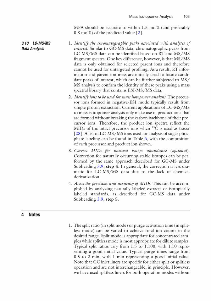
2. Identify ions to be used for mass isotopomer analysis. The precur-sor ions formed in negative-ESI mode typically result from simple proton extraction. Current applications of LC-MS/MS to mass isotopomer analysis only make use of product ions that are formed without breaking the carbon backbone of their pre-cursor ions. Therefore, the product ion spectra refl ect the MIDs of the intact precursor ions when 13 C is used as tracer [ 28 ]. A list of LC-MS/MS ions used for analysis of sugar phos-phate labeling can be found in Table 6 , with the composition of each precursor and product ion shown.

3. Correct MIDs for natural isotope abundance ( optional ) . Correction for naturally occurring stable isotopes can be per-formed by the same approach described for GC-MS under Subheading 3.9 , step 4 . In general, the correction is less dra-matic for LC-MS/MS data due to the lack of chemical derivatization.

4. Assess the precision and accuracy of MIDs. This can be accom-plished by analyzing naturally labeled extracts or isotopically labeled standards, as described for GC-MS data under Subheading 3.9 , step 5 .

4 Notes

1. The split ratio (in split mode) or purge activation time (in split-less mode) can be varied to achieve total ion counts in the desired range. Split mode is appropriate for concentrated sam-ples while splitless mode is most appropriate for dilute samples. Typical split ratios vary from 1:5 to 1:100, with 1:10 repre-senting a good initial value. Typical purge times range from 0.5 to 2 min, with 1 min representing a good initial value. Note that GC inlet liners are specifi c for either split or splitless operation and are not interchangeable, in principle. However, we have used splitless liners for both operation modes without

3.10 LC-MS/MS Data Analysis


104

noticeable deterioration in performance. Also note that when using splitless mode, the initial column temperature should be near or below the boiling point of the solvent in which the sample is dissolved [ 6 ].

2. The optimal linear velocity is in the range 20–40 cm/s for helium. Agilent’s FlowCalc tool or the instrument control software can help determine what the linear velocity will be for a particular combination of fl owrate, column diameter, tem-perature, and pressure.

3. The methoxyamine (MOX) reaction protects ketone and alde-hyde functional groups, and thereby prevents the formation of multiple TBDMS derivatives. This step is unnecessary if no ketone or aldehyde functional groups are present in the ana-lytes of interest. In this case, dissolve the dried sample in 50 μL anhydrous pyridine and skip Subheading 3.5 , step 3 .

Table 6 LC-MS/MS ions of sugar phosphates observed in cyanobacterial cell extracts

Metabolite [M−H] – Carbons Composition Production

2PG 155 1-2 C 2 H 4 O 6 P PO 3 −

2/3PGA 185 1-2-3 C 3 H 6 O 7 P PO 3 −

DHAP 169 1-2-3 C 3 H 6 O 6 P H 2 PO 4 −

E4P 199 1-2-3-4 C 4 H 8 O 7 P H 2 PO 4 −

F6P 259 1-2-3-4-5-6 C 6 H 12 O 9 P H 2 PO 4 −

FBP 339 1-2-3-4-5-6 C 6 H 13 O 12 P 2 H 2 PO 4 −

G6P 259 1-2-3-4-5-6 C 6 H 12 O 9 P H 2 PO 4 −

GAP 169 1-2-3 C 3 H 6 O 6 P H 2 PO 4 −

PEP 167 1-2-3 C 3 H 4 O 6 P PO 3 −

R5P 229 1-2-3-4-5 C 5 H 10 O 8 P H 2 PO 4 −

RuBP 309 1-2-3-4-5 C 5 H 11 O 11 P 2 H 2 PO 4 −

S7P 289 1-2-3-4-5-6-7 C 7 H 14 O 10 P H 2 PO 4 −

Ru5P 229 1-2-3-4-5 C 5 H 10 O 8 P H 2 PO 4 −

X5P 229 1-2-3-4-5 C 5 H 10 O 8 P H 2 PO 4 −

MS ions recommended for isotopomer analysis. Nominal masses, carbon backbone atoms, and molecular composition of each ion are listed. See Note 14 for metabo-lite abbreviations. The compositions of precursor and product ions are shown


105

4. Although polar phases are preferred for lipid analysis due to their enhanced resolving power, standard nonpolar phases have also been used successfully for less stringent separations.

5. In order to dissolve tributylamine completely in water, the tri-butylamine and acetic acid are fi rst mixed together in a dry fl ask before the requisite amount of ultrapure water is added. The solution is then fi ltered through a 0.45 μm membrane prior to use. The fi nal pH should be 4.5–5.

6. To increase sensitivity, the method should be divided into mul-tiple time segments with different MRM transitions scanned in each interval. Dwell time of each transition should be opti-mized such that the total cycle time in each time segment does not exceed 2 s. This will provide at least 10–15 scans of each chromatographic peak as it elutes from the column.

7. Two popular freeware programs for LC-MS/MS data analysis are MZmine and XCMS, the latter of which runs in the R sta-tistical programming environment. Both programs require the user to convert raw data fi les into a nonproprietary format such as mzXML, NetCDF, or mzData. Conversion to mzXML for-mat can be accomplished using one of several instrument- specifi c software tools developed and maintained by the Seattle Proteome Center ( http://tools.proteomecenter.org/software.php ).

8. Typically, this pellet is what remains after performing previous extractions to remove oil, protein, and free metabolites. Refer to Allen et al. [ 11 ] for details.

9. This step may be necessary for dilute samples in order to ensure complete conversion. However, it may be skipped for concen-trated samples.

10. Ensure tube lid remains secure. Periodically check to ensure that solution is in contact with pellet and hasn’t condensed on the lid of the tube. Shake liquid down if it has.

11. In some instances, a gel-like precipitate forms that requires additional time to dissolve. Leave overnight to fully dissolve, if necessary.

12. Many software packages will integrate ion chromatograms, but they often differ in the way they select the time-window of integration and perform baseline correction for each mass peak. If these parameters are not determined consistently for all mass isotopomers of a given fragment ion, substantial errors in the MID can occur (e.g., see Antoniewicz et al. [ 20 ]). This will give unacceptable results when performing the error analysis of Subheading 3.9 , step 5 . Therefore, choose an integration algorithm that is known to produce consistent datasets and has been validated using samples of known isotope labeling.


http://tools.proteomecenter.org/software.php

http://tools.proteomecenter.org/software.php

106

13. There are slight variations in natural 13 C-enrichment depend-ing upon the process of carbon fi xation utilized [ 29 ]. Plant RuBisCO exhibits a kinetic preference for 12 C over 13 C, with the effect being more pronounced in C3 plants relative to C4 plants [ 27 ]. However, the differences are in the range of 0.01–0.03 mol%, which are not measurable by typical quadru-pole MS instruments and therefore are insignifi cant in most MFA studies. These variations are only important when using GC-isotope ratio mass spectrometry (GC-IRMS) or similar approaches that provide highly accurate mass isotopomer measurements.

14. Abbreviations: 2PG , 2-phosphoglycolate; 2PGA , 2- phosphoglycerate; 3PGA , 3-phosphoglycerate; Akg , alpha- ketoglutarate; Cit , citrate; DHAP , dihydroxyacetone phos-phate; E4P , erythrose 4-phosphate; F6P , fructose-6-phosphate; FBP , fructose 1,6-bisphosphate; Fum , fumarate; G6P , glu-cose 6-phosphate; GAP , glyceraldehyde 3-phosphate; Lac , lactate; Mal , malate; Oac , oxaloacetate; PEP , phosphoenol-pyruvate; Pyr , pyruvate; R5P , ribose 5-phosphate; Ru5P , ribulose 5-phosphate; RuBP , ribulose 1,5-bisphosphate; S7P , sedoheptulose 7-phosphate; Suc , succinate; X5P , xylulose 5-phosphate.

15. Gln and Asn are converted to Glu and Asp during acid hydro-lysis and cannot be measured individually in protein hydroly-sates. However, they can be measured as free amino acids in cell extracts.

16. Although the McLafferty rearrangement ion at m/z 74 has been used extensively as a proxy of plastidic acetyl-CoA labeling, it should be treated with caution due to interfer-ences that can lead to signifi cant errors in the MID measure-ment. For example, Lonien and Schwender [ 30 ] have addressed this problem by adjusting the EI voltage to 15 eV from the standard 70 eV to reduce interference and by apply-ing statistical corrections to improve the accuracy of MID measurements.

Acknowledgments

This work has been supported by NSF CAREER Award CBET- 0955251 (to J.D.Y).


107

References

1. Sauer U (2006) Metabolic networks in motion: 13 C-based fl ux analysis. Mol Syst Biol 2:62

2. Zamboni N, Fendt SM, Ruhl M, Sauer U (2009) (13)C-based metabolic fl ux analysis. Nat Protoc 4:878–892

3. Paula Alonso A, Dale VL, Shachar-Hill Y (2010) Understanding fatty acid synthesis in developing maize embryos using metabolic fl ux analysis. Metab Eng 12:488–497

4. Yang C, Hua Q, Shimizu K (2002) Metabolic fl ux analysis in Synechocystis using isotope dis-tribution from 13C-labeled glucose. Metab Eng 4:202–216

5. Allen D, Ratcliffe R (2009) Quantifi cation of isotope label. In: Schwender J (ed) Plant Metabolic Networks . Springer, New York, pp 105–149

6. Kitson FG, Larsen BS, McEwen CN (1996) Gas chromatography and mass spectrometry : a practical guide. Academic, San Diego

7. Wolfe RR, Chinkes DL (2005) Isotope Tracers in Metabolic Research: Principles and Practice of Kinetic Analysis. Wiley, Hoboken, NJ

8. Lu W, Bennett BD, Rabinowitz JD (2008) Analytical strategies for LC-MS-based targeted metabolomics. J Chromatogr B Analyt Technol Biomed Life Sci 871:236–242

9. Dauner M, Sauer U (2000) GC-MS analysis of amino acids rapidly provides rich information for isotopomer balancing. Biotechnol Prog 16:642–649

10. Young JD, Walther JL, Antoniewicz MR, Yoo H, Stephanopoulos G (2008) An elementary metabolite unit (EMU) based method of iso-topically nonstationary fl ux analysis. Biotechnol Bioeng 99:686–699

11. Allen DK, Shachar-Hill Y, Ohlrogge JB (2007) Compartment-specifi c labeling information in 13C metabolic fl ux analysis of plants. Phytochemistry 68:2197–2210

12. Zamboni N, Sauer U (2009) Novel biological insights through metabolomics and 13C-fl ux analysis. Curr Opin Microbiol 12:553–558

13. Luo B, Groenke K, Takors R, Wandrey C, Oldiges M (2007) Simultaneous determina-tion of multiple intracellular metabolites in glycolysis, pentose phosphate pathway and tri-carboxylic acid cycle by liquid chromatography- mass spectrometry. J Chromatogr A 1147:153–164

14. Ausloos P, Clifton CL, Lias SG, Mikaya AI, Stein SE, Tchekhovskoi DV, Sparkman OD, Zaikin V, Zhu D (1999) The critical evaluation

of a comprehensive mass spectral library. J Am Soc Mass Spectrom 10:287–299

15. Kopka J, Schauer N, Krueger S, Birkemeyer C, Usadel B, Bergmuller E, Dormann P, Weckwerth W, Gibon Y, Stitt M, Willmitzer L, Fernie AR, Steinhauser D (2005) [email protected]: the Golm Metabolome Database. Bioinformatics 21:1635–1638

16. Kind T, Wohlgemuth G, Lee do Y, Lu Y, Palazoglu M, Shahbaz S, Fiehn O (2009) FiehnLib: mass spectral and retention index libraries for metabolomics based on quadru-pole and time-of-fl ight gas chromatography/mass spectrometry. Anal Chem 81:10038–10048

17. Smith CA, O’Maille G, Want EJ, Qin C, Trauger SA, Brandon TR, Custodio DE, Abagyan R, Siuzdak G (2005) METLIN: a metabolite mass spectral database. Ther Drug Monit 27:747–751

18. Wishart DS, Tzur D, Knox C, Eisner R, Guo AC, Young N, Cheng D, Jewell K, Arndt D, Sawhney S, Fung C, Nikolai L, Lewis M, Coutouly MA, Forsythe I, Tang P, Shrivastava S, Jeroncic K, Stothard P, Amegbey G, Block D, Hau DD, Wagner J, Miniaci J, Clements M, Gebremedhin M, Guo N, Zhang Y, Duggan GE, Macinnis GD, Weljie AM, Dowlatabadi R, Bamforth F, Clive D, Greiner R, Li L, Marrie T, Sykes BD, Vogel HJ, Querengesser L (2007) HMDB: the Human Metabolome Database. Nucleic Acids Res 35:D521–D526

19. Horai H, Arita M, Kanaya S, Nihei Y, Ikeda T, Suwa K, Ojima Y, Tanaka K, Tanaka S, Aoshima K, Oda Y, Kakazu Y, Kusano M, Tohge T, Matsuda F, Sawada Y, Hirai MY, Nakanishi H, Ikeda K, Akimoto N, Maoka T, Takahashi H, Ara T, Sakurai N, Suzuki H, Shibata D, Neumann S, Iida T, Funatsu K, Matsuura F, Soga T, Taguchi R, Saito K, Nishioka T (2010) MassBank: a public reposi-tory for sharing mass spectral data for life sci-ences. J Mass Spectrom 45:703–714

20. Antoniewicz MR, Kelleher JK, Stephanopoulos G (2007) Accurate assessment of amino acid mass isotopomer distributions for metabolic fl ux analysis. Anal Chem 79:7554–7559

21. Price NP (2004) Acylic sugar derivatives for GC/MS analysis of 13C-enrichment during carbohydrate metabolism. Anal Chem 76:6566–6574

22. Antoniewicz MR (2006) Comprehensive Analysis of Metabolic Pathways Through the


108

Combined Use of Multiple Isotopic Tracers, In Chemical Engineering , p 370. Massachusetts Institute of Technology, Cambridge, MA

23. Christie WW (1993) Preparation of ester deriv-atives of fatty acids for chromatographic analy-sis. Advances in lipid methodology 2:69–111

24. Yang L, Kasumov T, Yu L, Jobbins KA, David F, Previs SF, Kelleher JK, Brunengraber H (2006) Metabolomic assays of the concentra-tion and mass isotopomer distribution of glu-coneogenic and citric acid cycle intermediates. Metabolomics 2:85–94

25. Shastri AA (2008) Metabolic fl ux analysis of photosynthetic systems, In School of Chemical Engineering . Purdue University, West Lafayette, IN

26. Fernandez CA, Des Rosiers C, Previs SF, David F, Brunengraber H (1996) Correction of 13C mass isotopomer distributions for nat-ural stable isotope abundance. J Mass Spectrom 31:255–262

27. Coplen T, Böhlke J, De Bievre P, Ding T, Holden N, Hopple J, Krouse H, Lamberty A, Peiser H, Revesz K (2002) Isotope-abundance variations of selected elements:(IUPAC tech-nical report). Pure Applied Chem 74:1987–2017

28. Kiefer P, Nicolas C, Letisse F, Portais JC (2007) Determination of carbon labeling dis-tribution of intracellular metabolites from sin-gle fragment ions by ion chromatography tandem mass spectrometry. Anal Biochem 360:182–188

29. Berg IA, Kockelkorn D, Ramos-Vera WH, Say RF, Zarzycki J, Hugler M, Alber BE, Fuchs G (2010) Autotrophic carbon fi xation in archaea. Nat Rev Microbiol 8:447–460

30. Lonien J, Schwender J (2009) Analysis of met-abolic fl ux phenotypes for two Arabidopsis mutants with severe impairment in seed stor-age lipid synthesis. Plant Physiol 151:1617–1634


Documents

Chapter 7 · 85 Ganesh Sriram (ed.), Plant Metabolism: Methods and Protocols , Methods in Molecular Biology, vol. 1083, ... Jamey oung , Y