Chapter 7 High Dimensional Problems

Chapter 7

High DimensionalProblems

In observationalstudiesweusuallyhaveobservedpredictorsorcovariates��

andaresponsevariable� . A scientistis interestedin therelationbetweentheco-variatesandtheresponse,astatisticiansummarizestherelationshipwith�� ! "�

(7.1)

Knowing theaboveexpectationhelpsus# understandtheprocessproducing�# assesstherelativecontributionof eachof thepredictors# predictthe � for somesetof values��$

.

Oneexampleis theair pollution andmortality data. Theresponsevariable � isdaily mortality counts. Covariatesthat aremeasuredaredaily measurementsofparticulateair pollution

��, temperature

�$�, humidity

�$%, andotherpollutants�!&

,. . . ,�'

.

Note: In this particularexamplewe canconsiderthepastascovariates.GAM ismoreappropriatefor datafor which thisdoesn’t happen.

83

84 CHAPTER7. HIGH DIMENSIONAL PROBLEMS

In thissectionwewill belookingatadiabetesdatasetwhichcomesfrom astudyof thefactorsaffectingpatternsin insulin-dependentdiabetesmellitusin children.Theobjectivewasto investigatethedependenceof thelevelof serumC-peptideonvariousotherfactorsin orderto understandthepatternsof residualinsulin secre-tion. Theresponsemeasurements� is the logarithmof C-peptideconcentration(mol/ml) at diagnosis,andthepredictormeasurementsareageandbasedeficit,ameasurementof acidity.

A modelthathastheform of (7.1)andis oftenusedis� ��! "�)(+*(7.2)

with*

a randomerror with mean0 and variance , � independentfrom all the�� .

Usually we make a further assumption,that*

is normally distributed. Now wearenot only sayingsomethingaboutthe relationshipbetweenthe responseandcovariatesbut alsoaboutthedistributionof � .

Givensomedata,“estimating”��-.��-/ "�

canbe“hard”. Statisticianslike tomake it easyassuminga linearregressionmodel�0�1��! "��32�(546�7��)(8�9(54: �� This is usefulbecauseit# is verysimple# summarizesthecontributionof eachpredictorwith onecoefficient# providesaneasyway to predict � for asetof covariates

��! .

It is notcommonto haveanobservationalstudywith continuouspredictorswherethereis “science”justifying this model. In many situationsit is moreuseful tolet the data“say” what the regressionfunction is like. We may want to stayawayfrom linearregressionbecauseit forceslinearityandwemayneverseewhat��-.��-/ "�

is really like.

85

In thediabetesexamplewegetthefollowing result:

•

•

•

•

•

• •

•

•

•

•

•

••

•

•

•

•

•

•

•

•

•

•

•

••

•

••

•

••

•

•

• •

•

•

•

•

••

Age;

log(

C.P

eptid

e)

5<

10 15

1.2

1.4

1.6

1.8

•

•

•

•

•

••

•

•

•

•

•

••

•

•

•

•

•

•

•

•

•

•

•

••

•

••

•

••

•

•

• •

•

•

•

•

••

Base.Deficit=

log(

C.P

eptid

e)

-30 -25 -20 -15 -10 -5 0>1.

21.

41.

61.

8

Sodoesthedataagreewith thefits? Let’sseeif a “smoothed”versionof thedataagreeswith this result.

But how do we smooth?Someof the smoothingprocedureswe have discussedmaybegeneralizedto caseswherewe havemultiplecovariates.

Therearewaysto definesplinessothat ?�@:A�BDC FE C . Weneedto defineknotsin AGBHC andrestrictionson themultiple partialderivativewhich is difficult butcanbedone.

It is mucheasierto generalizeloess.The only differenceis that therearemanymorepolynomialsto choosefrom:

4/IJ��4/IK(G46�L-M�N4/IK(�46�7-O(G4/��PQ�N4/IR(G46�7-S(G4/�NPT(4/%N-UPV��4/I0(W46�7-!(W4/�NPX(W4/%N-UPY(54K&�- �, etc...


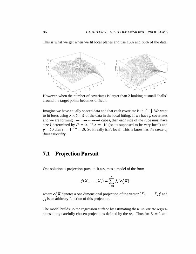
This is whatwe getwhenwe fit local planesanduse15%and66%of the data.

2Z 4

6[ 8\ 10] 12] 14]

Age-25

-20

-15

-10

-5

Base Deficit

^ 00.

51

1.5

22.

5P

redi

cted

2_ 4

6` 8a 10b 12b 14b

Age-25

-20

-15

-10

-5

Base Deficit

c1.2

1.3

1.4

1.5

1.6

1.7

Pre

dict

ed

However, whenthenumberof covariatesis largerthan2 looking at small“balls”aroundthetargetpointsbecomesdifficult.

Imaginewehaveequallyspaceddataandthateachcovariateis in dfe �g�h . Wewantto fit loessusing ikj g e"e:l of thedatain thelocal fitting. If wehave m covariatesandweareforming mXnGo:prq�st)uprv�t6wyx cubes,theneachsideof thecubemusthavesize x determinedby x � i . If i �z{g e (so its supposedto be very local) andm �|g e then x �|{g �~}��I �|��

. Soit really isn’t local! This is known asthecurseofdimensionality.

7.1 Projection Pursuit

Onesolutionis projection-pursuit.It assumesa modelof theform��1��$ "�T� � � � � � ��where

� ��denotesaonedimensionalprojectionof thevector

�1�� 9� �and� �

is anarbitraryfunctionof thisprojection.

Themodelbuilds up theregressionsurfaceby estimatingtheseunivariateregres-sionsalongcarefullychosenprojectionsdefinedby the

��. Thusfor � ��g

and

7.2. ADDITIVE MODELS 87m ��the regressionsurfacelooks like a corrugatedsheetandis constantin the

directionsorthogonalto2M�

.

If you don’t seehow this solvesthe problemof dimensionality, the next sectionwill helpyouunderstand.

7.2 Additi veModels

Additive modelsare specificapplicationof projectionpursuit. They are moreusefulin scientificapplications.

In additive modelswe assumethattheresponseis linear in thepredictorseffectsand that there is an additive error. This allows us to study the effect of eachpredictorseparately. Themodelis like (7.2)with�� 1� � ��Noticethatthis is projectionpursuitwith theprojection�� Theassumptionmadehereis notasstrongasin linearregression,but its still quitestrong.It’ssayingthattheeffectof eachcovariateis additive. In practicethismaynotmakesense.

Example:In thediabetesexampleconsideranadditivemodelthatmodelslog(C-peptide)in termsof age

��andbasedeficit

�$�. The additive modelassumes

that for two differentages-.�

and- � �

theconditionalexpectationof � (seenasarandomvariabledependingonbasedeficit):

E� �� -.��H�:��-.��)(��J�1�$��

andE� �� 8- � � ��$��"��1- � � �)(��


Thissaythattheway C-peptidedependson basedeficit only variesby a constantfor differentages.It is not easyto disregardthepossibility that this dependencechanges.For example,atolderagestheeffectof high basedeficit canbedramat-ically bigger. However, in practicewe have too make assumptionslike theseinorderto getsomekind of usefuldescriptionof thedata.

Comparingthenon-additivesmooth(seenabove) andtheadditivemodelsmoothshowsthatit is notcompletelycrazyto assumeadditivity.

2� 4� 6� 8� 10� 12� 14�

Age-25

-20

-15-10

-5

Base Deficit

�1.21

.31.

41.5

1.61

.7P

redi

cted

2� 4 6¡ 8¢ 10£ 12£ 14£

Age-25

-20

-15-10

-5

Base Deficit

¤1.21

.31.

41.5

1.61

.7P

redi

cted

Noticethatin thefirst plotsthecurvesdefinedfor thedifferentagesaredifferent.In thesecondplot they areall thesame.

How did we createthis lastplot? How did wefit theadditivesurface.We needtoestimate

�:�and

�9�. Wewill seethis in thenext section.

Noticethatoneof theadvantagesof additivemodelis thatnomatterthedimension

7.2. ADDITIVE MODELS 89

of thecovariatesweknow whatthesurface�� 9�

is likeby drawing each� � �1� � �separately.

•

•

•

•

•

• •

•

•

•

•

•

••

•

•

•

•

•

•

•

•

•

•

•

••

•

••

•

••

•

•

• •

•

•

•

•

••

Age;

log(

C.P

eptid

e)

5<

10 15

1.2

1.4

1.6

1.8

•

•

•

•

•

••

•

•

•

•

•

••

•

•

•

•

•

•

•

•

•

•

•

••

•

••

•

••

•

•

• •

•

•

•

•

••

Base.Deficit=

log(

C.P

eptid

e)

-30 -25 -20 -15 -10 -5 0>1.

21.

41.

61.

8

7.2.1 Fitting Additi ve Models: The Backfitting Algorithm

Conditionalexpectationsprovide a simpleintuitivemotivationfor thebackfittingalgorithm.

If theadditivemodelis correctthenfor any ¥E

¦ �§n 2 n � �¨� � � � �� ©©©©© � ��ª �� Thissuggestaniterativealgorithmfor computingall the

� �.

Why? Let’s say we have estimates «�:�� «�� ¬/� andwe think they are “good”


estimatesin thesensethatE

� � � �1� � � n � � �� is “closeto 0”. Thenwehavethat

E

¦ ��n «2 n ¬/�� «� � �1� � ��©©©©© �� ª® �� y�� Thismeansthatthepartialresiduals«¯ � �§n «2 n5° ¬/�� «� � �1� � �«¯�± �� y�1� ± 9�)(5² ±with the

² ± approximatelyIID mean0 independentof the��

’s. We have alreadydiscussedvarious“smoothing” techniquesfor estimating

�� in a model as the

above.

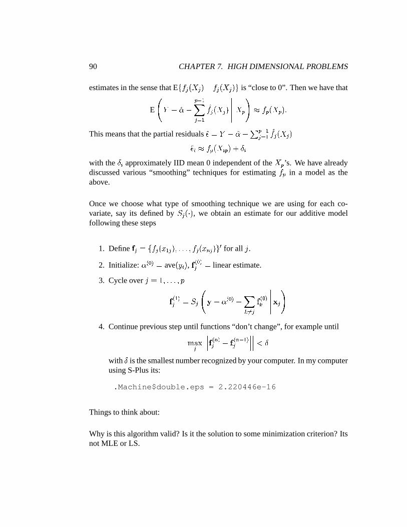
Oncewe choosewhat type of smoothingtechniquewe are using for eachco-variate,say its definedby ³ � �µ´¶� , we obtainan estimatefor our additive modelfollowing thesesteps

1. Define · � � � � � �1-.� � �� 1-/ � � � �for all ¸ .

2. Initialize:2T¹ I»º �

ave�1P ± � , · ¹ I»º� �

linearestimate.

3. Cycleover ¸ �¼g"�� m· ¹ �~º� � ³ � ¦¾½ n 2 ¹ I»º n � �9¨� � · ¹ I»º� ©©©©©�¿ ��ª4. Continuepreviousstepuntil functions“don’t change”,for exampleuntilÀ�Á�Â� ©©© ©©© · ¹ º� nÃ· ¹ �¬/�~º� ©©© ©©©/Ä ²

with²

is thesmallestnumberrecognizedbyyourcomputer. In mycomputerusingS-Plusits:

.Machine$double.eps = 2.220446e-16

Thingsto think about:

Why is thisalgorithmvalid? Is it thesolutionto someminimizationcriterion?ItsnotMLE or LS.


7.2.2 Justifying the backfitting algorithm

Thebackfittingalgorithmseemsto makesense.Wecansaythatwehavegivenanintuitive justification.

However statisticiansusuallylike to have morethanthis. In mostcaseswe canfind a “rigorous” justification. In many casestheassumptionsmadefor the“rig-orous” justificationstoo work arecarefullychosenso thatwe get theanswerwewant,in this casethat theback-fittingalgorithm“converges”to the“correct” an-swer.

In the GAM book,H&T find threewaysto justify it: Finding projectionsin Å �function spaces,minimizing certaincriterion with solutionsfrom reproducing-kernelHilbert spaces,andasthesolutionto penalizedleastsquares.Wewill lookat this lastone.

We extendtheideaof penalizedleastsquaresby consideringthefollowing crite-rion � ± � ��Æ P ± n � � � � � � ��- ± � ��Ç � ( � � � � i �6ÈH� � � �� 1É�� o Éoverall p-tuplesof functions

�~�:�� thataretwicedifferentiable.

As beforewe can show that the solution to this problemis a p-tuple of cubicsplineswith knots“at thedata”,thuswemayrewrite thecriterionas¦V½ n � � � � · ��ª

� ¦V½ n � � � � · ��ª ( � � � � i � · ��Ê�� · �wherethe

Ê��s arepenaltymatricesfor eachpredictordefinedanalogouslyto the

Êof section3.3.

If we differentiatethe above equationwith respectto the function · � we obtainn �Ë� ½ n¼° � · � �Ì(®� i ��Ê�� · � � e . The «· � ’s that solve the above equationmust


satisfy: «· � �Í��ÎT( i ��Ê�� ¬/� ¦ ½ n � �J¨� � «· � ª � ¸ �¼g"�� mIf we definethe smootheroperator Ï � � �1ÎT( i ��Ê�� ¬/� we can write out thisequationin matrixnotationasÐÑÑÑÒ Î Ï �Ó� Ï �Ï � Î � Ï �

......

......Ï Ï � ÎÔ�ÕÕÕÖ ÐÑÑÑÒ · �· �

...· Ô�ÕÕÕÖ � ÐÑÑÑÒ Ï � ½Ï � ½

...Ï ½Ô�ÕÕÕÖ

Onewayto solvethisequationis to usetheGauss-Seidelalgorithmwhich in turnis equivalentto solvingtheback-fittingalgorithm.SeeBuja,Hastie& Tibshirani(1989)Ann. Stat.17,435–555for details.

Rememberthatthatfor any setof linearsmoother«· � � Ï � ½we canarguein reversethatit minimizessomepenalizedleastsquarescriteriaoftheform � ½ n �×� · � � � � ½ n �"� · � �)( �:� · �� Ï ¬� nÃA � · �andconcludethatit is thesolutionto somepenalizedleastsquaredproblem.

7.2.3 Standard Err or

Whenusinggam() in S-Pluswe getpoint-wisestandarderrors. How aretheseobtained?

Notice thatour estimates«· � areno longerof the form Ï � ½ sincewe have usedacomplicatedbackfittingalgorithm. However, at convergencewe canexpress «· �as Ø � ½ for somet+jÙt matrix Ø � . In practicethis Ø � is obtainedfrom the lastcalculationof the «· � ’sbut findingaclosedform is rarelypossible.


Waysof constructingconfidencesetsis not straightforward,and(to the bestofmy knowledge)is anopenareaof research.


7.3 ClassificationAlgorithms and RegressionTrees

This is from thebookby Breimanet. al.

At the university of California, SanDiego Medical Center, whena heartattackpatientis admitted,19 variablesaremeasuredduringthefirst 24 hours.They in-cludeBP, ageand17otherbinarycovariatessummarizingthemedicalsymptomsconsideredasimportantindicatorsof thepatient’scondition.

The goal of a medicalstudy can be to develop a methodto identify high riskpatientson thebasisof theinitial 24-hourdata.

The next figure shows a pictureof a treestructuredclassificationrule that wasproducedin the study. The letter F meansno high andthe letter G meanshighrisk.

7.3. CLASSIFICATION ALGORITHMS AND REGRESSIONTREES 95

How canweusedatatoconstructtreesthatgiveususefulanswers.Thereis alargeamountof work donein this typeof problem.We will give a brief descriptioninthissection.

7.3.1 ClassifiersasPartitions

Supposewe havea categoricaloutcomeP�Ú�ÛÜ� � g"��R��Ý �

. We callÛ

thesetof classes.Denotewith Þ thespaceof all possiblecovariates.

We candefinea classificationrule asa function o � ¿ � definedon Þ so that forevery ¿ , o � ¿ � is equalto oneof thenumbers

g"��Ý.

This couldbeconsidereda systematicway of predictingclassmembershipfromthecovariates.

Anotherway to defineclassifiersis to partition Þ into disjoint sets ß �� ß �with o � ¿ �T� ¸ for all ¿ Ú ß � .But how doweconstructtheseclassifiersfrom data?

7.3.2 What is truth?

We are now going to describehow to constructclassificationrules from data.Thedatawe useto constructthe treeis calledthetrainingset à which is simply� � ¿ �� ¸ ��9� ¿ y� ¸ ×� � .Onceaclassificationrule o �1�Ü� is constructedhow dowedefineit’ saccuracy?

In thissectionwewill definethetruemisclassificationrate áXâ � o � .Onewayto estimateáXâ � o � is to draw anothervery largesubset(virtually infinite)


from thesamepopulationas à andobservetherateof correctclassificationin thatset.Theproportionmisclassifiedby o is ourestimateof áXâ � o � .To make this definition moreprecise,definethe spaceÞãj Û as the setof allcouples

� ¿ � ¸ � where¿ Ú Þ and ¸ ÚkÛ . Let ä�å � ß � ¸ � bea probabilitydistributionon Þæj Û . Assumeeachelementof à is aniid outcomefrom thisdistribution.

Wedefinethemisclassificationrateasá â � o �� ä�åJdfo � ¿ �Xç� ¸.� à h (7.3)

with� ¿ � ¸ � anoutcomeindependentof à .

How doweobtainanestimateof this?

The substitutionestimatesimply countshow many timeswe areright with thedatawehave, i.e. á � o �� gè é� � � gê ¹ìë�í º ¨� � í The problemwith this estimateis that most classificationalgorithmsconstructo trying to minimize the above equation. If we have enoughcovariateswe candefinearule thatalwayshaso � ¿ "�T� ¸ andrandomlyallocatesany other ¿ . Thishasan á � o �T� e but onecanseethat,in general,áXâ � o � will bemuchbigger.

Anotherpopularapproachis the testsampleestimate.Herewe divide thedata àinto two groupsà � and à � . We thenuse à � to define o and à � to estimateáXâ � o �with á � o �T� gè�� ë�í�î�ï:ð gê ¹�ë í º ¨� � íwith

è'�thesizeof à � . A popularchoicefor

è'�is 1/3 of

è, thesizeof à .

A problemwith thisprocedureis thatwedon’t use1/3of thedatawhenconstruct-ing o . In situationswhere

èis very largethismaynot besuchabig problem.

The third approachis crossvalidation. We divide the data into many subsetsof equal(or approximatelyequal)size à �� àSñ , definea o"ò for eachof these


groups,andusetheestimateá � o �T� gó ñ� ò � � gè ò �ë�í�î�ï"ô g ê ¹�ë í º ¨� � í 7.3.3 BayesRule

Themajorguidethathasbeenusedin theconstructionof classifiersis theconceptof theBayesrule. A Bayesrule is the o×õ for whichä�å9dfoyõ � ¿ �Xç� ¸ �Ìö ä�åJdfo � ¿ �Xç�8P×hrfor all classificationrules o � ¿ � .If weassumethat ä�å � ß$� ¸ � hasaprobabilitydensity

� � � ¿ � suchthatä�å � ß$� ¸ �� ÈK÷ � � � ¿ � o -thenwecanshow thato×õ � ¿ �T� ¸ on ß � � � ¿�ø � � � ¿ � ä�å � ¸ �� À�Á9Â± � ± � ¿ � äTå � ¸ � � Discriminantanalysis,kerneldensityestimation,and ¥ -thnearestneighborsmooth-ing attemptto estimate

� � � ¿ � and ä�å � ¸ � in orderto estimatetheBayesrule. Theymakemany assumptionssothemethodsarenot alwaysuseful.

7.3.4 Constructing tr eeclassifiers

Noticehow big the spaceof all possibleclassifiersis. In the simplecasewhereÞ � � e �g � thisspacehas�

elements.

Binary treesarea specialcaseof this partition. Binary treesareconstructedbyrepeatedsplitsof thesubsetsof Þ into two descendantsubsets,beginningwith Þitself.


ÞÌù ÞSú ÞSûÞSü ÞÌý

þþþþþ ÿ ÿ ÿ ÿ ÿ��

� � � � � �

��

� � � � � �

��

� � � � � �

ÞÞ � Þ %

Þ &

Split 1

Split 2 Split 3

Split 4

Thesubsetscreatedby thesplitsarecallednodes. Thesubsetswhicharenotsplitarecalledterminalnodes.

Eachterminalnodesgetsassignedto oneof the classes.So if we had3 classeswe couldget ß �Y� ÞÌù�� ÞÌý , ß �F� ÞÌú and ß % � ÞSû�� ÞÌü . If we areusingthedatawe assigntheclassmostfrequentlyfoundin thatsubsetof Þ . We call theseclassificationtress.

Variousquestionstill remainto beanswered# How dowedefinetruth?# How doweconstructthetreesfrom data?

7.3. CLASSIFICATION ALGORITHMS AND REGRESSIONTREES 99# How doweassesstrees,i.e. whatmakesagoodtree?

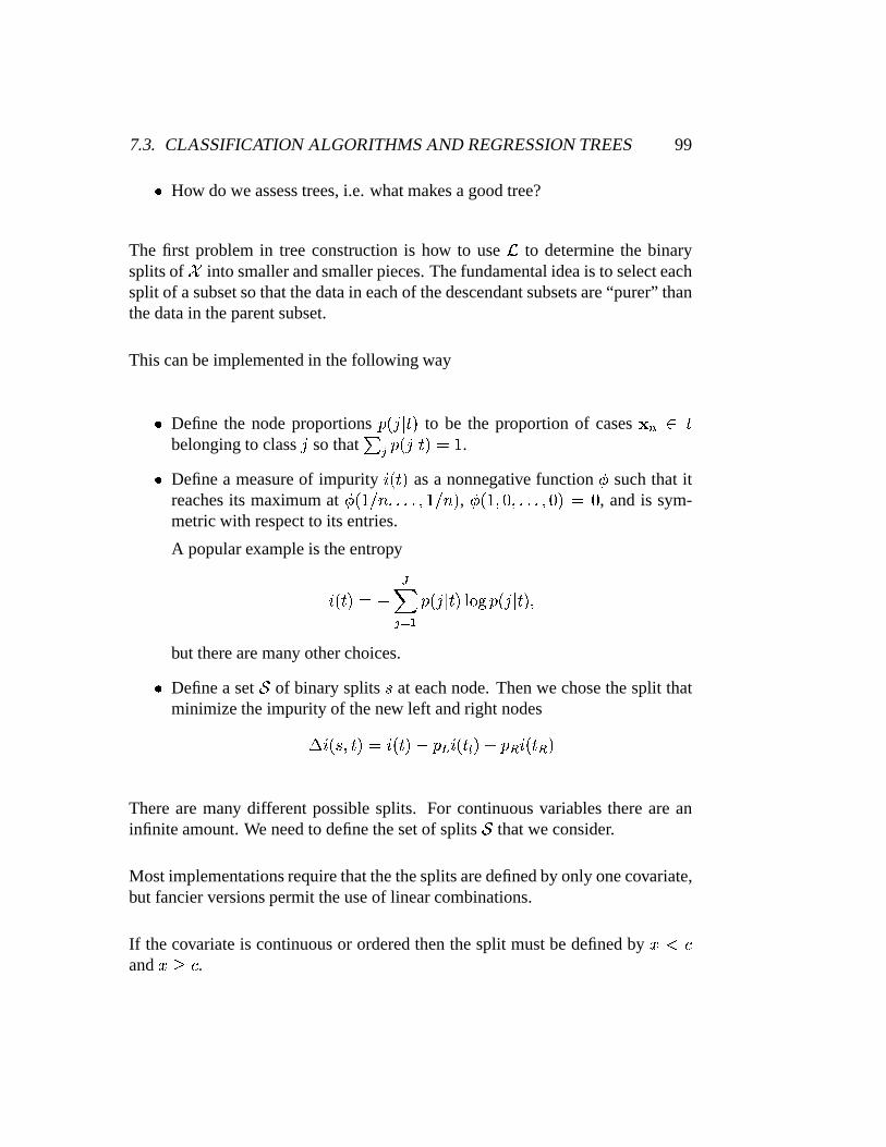
The first problemin treeconstructionis how to use à to determinethe binarysplitsof Þ into smallerandsmallerpieces.Thefundamentalideais to selecteachsplit of asubsetsothatthedatain eachof thedescendantsubsetsare“purer” thanthedatain theparentsubset.

Thiscanbeimplementedin thefollowing way# Define the nodeproportionsm � ¸.� É�� to be the proportionof cases¿ 3Ú Ébelongingto class sothat ° � m � ¸.� É��¼g

.# Definea measureof impurity p ��É�� asa nonnegative function � suchthat itreachesits maximumat � �»g�� t ��g�� t � , � �µg � e �� e � � e , andis sym-metricwith respectto its entries.

A popularexampleis theentropyp ��É��T� n �� m � ¸)� É�� m � ¸.� É��but therearemany otherchoices.# Definea set � of binarysplits u at eachnode.Thenwe chosethesplit thatminimizetheimpurity of thenew left andright nodes

� p � u ��É�� p �1É�� nkm��Rp �1É�� )( m��Up ��É � �Therearemany differentpossiblesplits. For continuousvariablesthereareaninfinite amount.Weneedto definethesetof splits � thatweconsider.

Most implementationsrequirethatthethesplitsaredefinedby only onecovariate,but fancierversionspermittheuseof linearcombinations.

If thecovariateis continuousor orderedthenthesplit mustbedefinedby- Ä �

and-�� .


If thecovariateis categoricalthenwesimplyconsiderall splitsthatdivideoriginalsetinto two.

1 2 1

2 3


� � � � � �

��

� � � � � �

��

� � � � � �

-.�-U� -U%

-U�Ä � � �

�� ö � �3� ç�� g ö§g

Now all we needis a stoppingrule andwe arereadyto createtrees. A simplestoppingrule is that

� p � u ��É�� Ä ² , but thisdoesnot work well in practice.

Whatis usuallydoneis thatwelet thetreesgrow to asizethatis biggerthanwhatwe think makessenseandthenprune.Weremovenodeby nodeandcomparethetreesusingestimatesof áXâ � o � .Sometimestosavetimeand/orchoosesmallertreeswedefineapenalizedcriterionbasedon áXâ � o � .


The big issuehereis modelselection. The modelselectionproblemconsistsoffour orthogonalcomponents.

1. Selecta spaceof models

2. Searchthroughmodelspace

3. Comparemodels# of thesamesize# of differentsizes(penalizecomplexity)

4. Assesstheperformanceof aprocedure

Important points:# Components2and3areoftenconfused(e.g.,in stepwiseregression).That’sbad.# Peopleoftenforgetcomponent1.# Peoplealmostalwaysignorecomponent4; it canbethehardest.

Bettertreesmaybefoundby doinga one-step“look ahead,” but this comeswiththecostof agreatincreasein computation.

7.3.5 RegressionTrees

If insteadof classificationwe are interestedin predictingwe canassigna pre-dictive valueto eachof the terminalnodes.Notice that this definesan estimatefor the regressionfunctionE

� �� ! � that is like a multidimensionalbinsmoother. Wecall theseregressiontrees.


Regressiontreesareconstructedin a similar way to classificationtrees.They areusedfor thecasewhere� is acontinuousrandomvariable.

A regressiontreepartitions--spaceinto disjoint regions ß � andprovidesa fitted

valueE�1P � -kÚ ß � � within eachregion.

13 34 77

51 26


� � � � � �

��

� � � � � �

��

� � � � � �

-.�-U� -U%

-U�Ä � � �

�� ö � �3� ç�� g ö§g

In otherwords,this is adecisiontreewheretheoutcomeis a fittedvalueforP.

Weneedanew definition o � ¿ � and áXâ � o � .Now o � ¿ � � will simplybetheaverageof theterminalnodewhere¿ � lies. So o � ¿ �definesastep-functionC E C .


Insteadof misclassificationrate,wecandefinemeansquarederrorá â � o �� E d ��nWo � ¿ �»h �Therestis prettymuchthesame.

7.3.6 Generalpoints

FromKarl Broman’snotes.# This is mostnaturalwhentheexplanatoryvariablesarecategorical (anditis especiallynicewhenthey arebinary).# Thereis nothingspecialaboutthe treestructure...thetreejust partitions

--

space,with afittedvaluein eachregion.# Advantage: Thesemodelsgoafterinteractionsimmediately, ratherthanasanafterthought.# Advantage: Treescanbeeasyto explain to non-statisticians.# Disadvantage: Tree-spaceis huge,sowemayneeda lot of data.# Disadvantage: It canbehardto assessuncertaintyin inferenceabouttrees.# Disadvantage: Theresultscanbequitevariable.(Treeselectionis notverystable.)# Disadvantage: Actual additivity becomesa messin a binary tree. Thisproblemis somewhatalleviatedby allowing splitsof theform

-.�0(��-U� Ä� �� o .Computing with tr ees

R: library(tree); library(rpart) [MASS, ch10]


An important issue: Storingtrees

Binarytreesarecomposedof nodes(rootnode,internalnodesandterminalnodes).

Rootandinternalnodes:# Splitting rule (variable+ whatgoesto right)# Link to left andright daughternodes# Possiblya link to theparentnode(null if this is therootnode)

Terminalnodes:# Fittedvalue# Possiblya link to theparentnode

C: Usepointersandstructures(struct)

R: It beatsme.Takea look.

Ref: Breimanetal (1984)Classificationandregressiontrees.Wadsworth.

Documents

Chapter 7 High Dimensional Problems