Chapter 7 Magnetostatic

7/30/2019 Chapter 7 Magnetostatic

http://slidepdf.com/reader/full/chapter-7-magnetostatic 1/45

1

CHAPTER 7MAGNETOSTATIC FIELDS



2

LECTURE SYLLABUS

•

INTRODUCTION• BIOT-SAVART’S LAW

• AMPERE’S CIRCUIT LAW-MAXWELL’SEQUATION

• APPLICATIONS OF AMPERE’S LAW

• MAGNETIC FLUX DENSITY-MAXWELL’SEQUATION

• MAXWELL’S EQUATION FOR STATIC FIELDS

• MAGNETIC SCALAR & VECTOR POTENTIALS• DERIVATION OF BIOT-SAVART’S LAW &

AMPERE’S LAW



3

7.1 INTRODUCTION

• Static magnetic fields are characterized by H and B such as E and D

on electrostatic fields.

• There are similarities and dissimilarities between electric and

magnetic fields. Example the relation between H and B are H = B

and relation between E and D are related according to D = E. Table

7.1 further shows the analogy between electric and magnetic fieldquantities.

• Missing link - thanks to Oersted (1820).

• An electrostatic field is produced by static or stationary charges. If

the charges are moving with constant velocity, a static magnetic field

is produced. A magnetostatic field is produced by a constant currentflow.



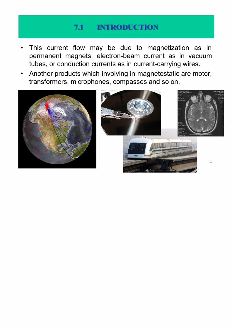
• This current flow may be due to magnetization as in

permanent magnets, electron-beam current as in vacuum

tubes, or conduction currents as in current-carrying wires.

• Another products which involving in magnetostatic are motor,

transformers, microphones, compasses and so on.

4

7.1 INTRODUCTION



5

Table 7.1



6

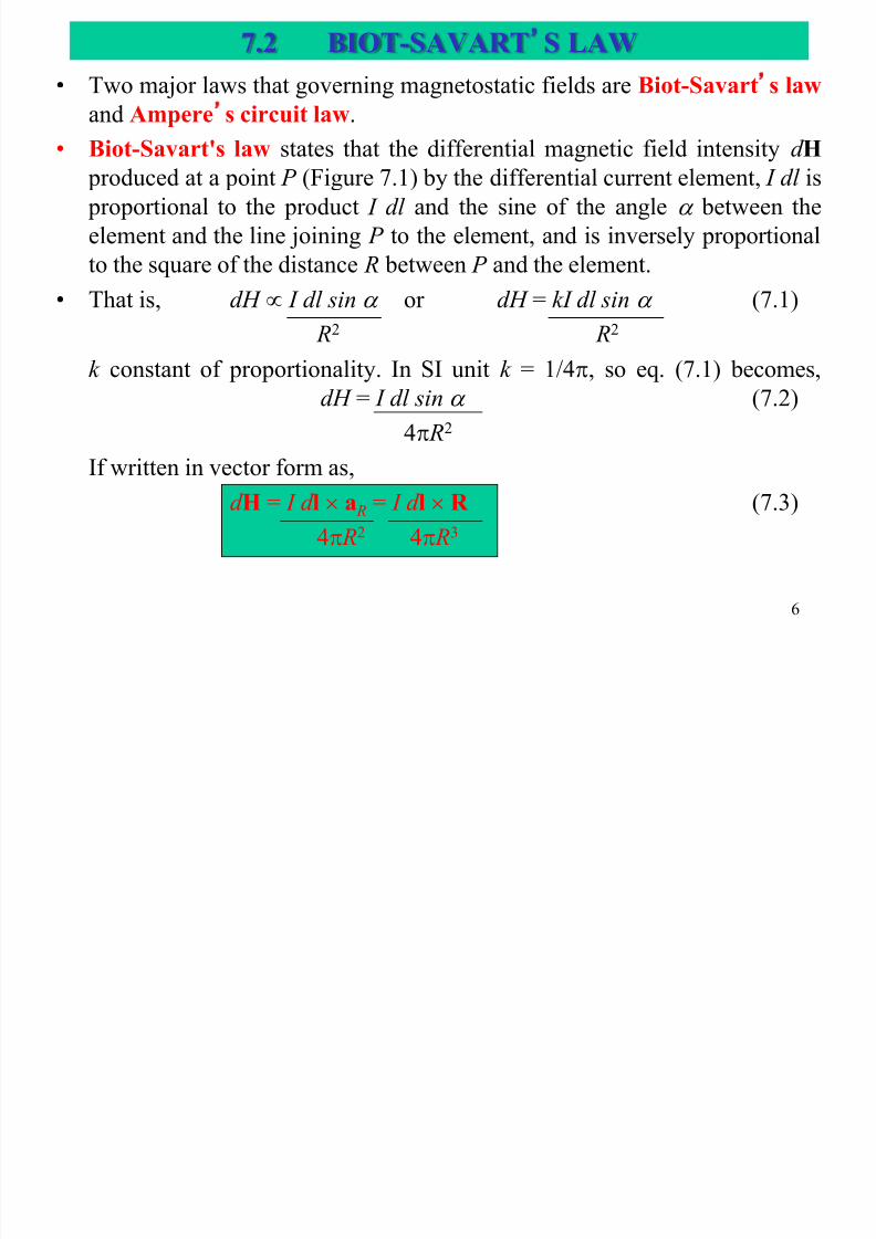
7.2 BIOT-SAVART’S LAW

• Two major laws that governing magnetostatic fields are Biot-Savart’s law

and Ampere’s circuit law.

• Biot-Savart's law states that the differential magnetic field intensity d H produced at a point P (Figure 7.1) by the differential current element, I dl is

proportional to the product I dl and the sine of the angle between the

element and the line joining P to the element, and is inversely proportional

to the square of the distance R between P and the element.

• That is, dH I dl sin or dH = kI dl sin (7.1) R2 R2

k constant of proportionality. In SI unit k = 1/4, so eq. (7.1) becomes,

dH = I dl sin (7.2)

4 R2

If written in vector form as,

d H = I d l a R = I d l R (7.3)

4 R2 4 R3



7

Figure 7.1

Right hand rule Right handed screw rule

Figure 7.3

Figure 7.2



CONCEPT QUESTION #1

The magnetic field at point P

points towards the:

a) +x direction

b) -x direction

c) +y direction

d) -y directione) +z direction

f) -z direction

g) field is zero (no direction)

8

x



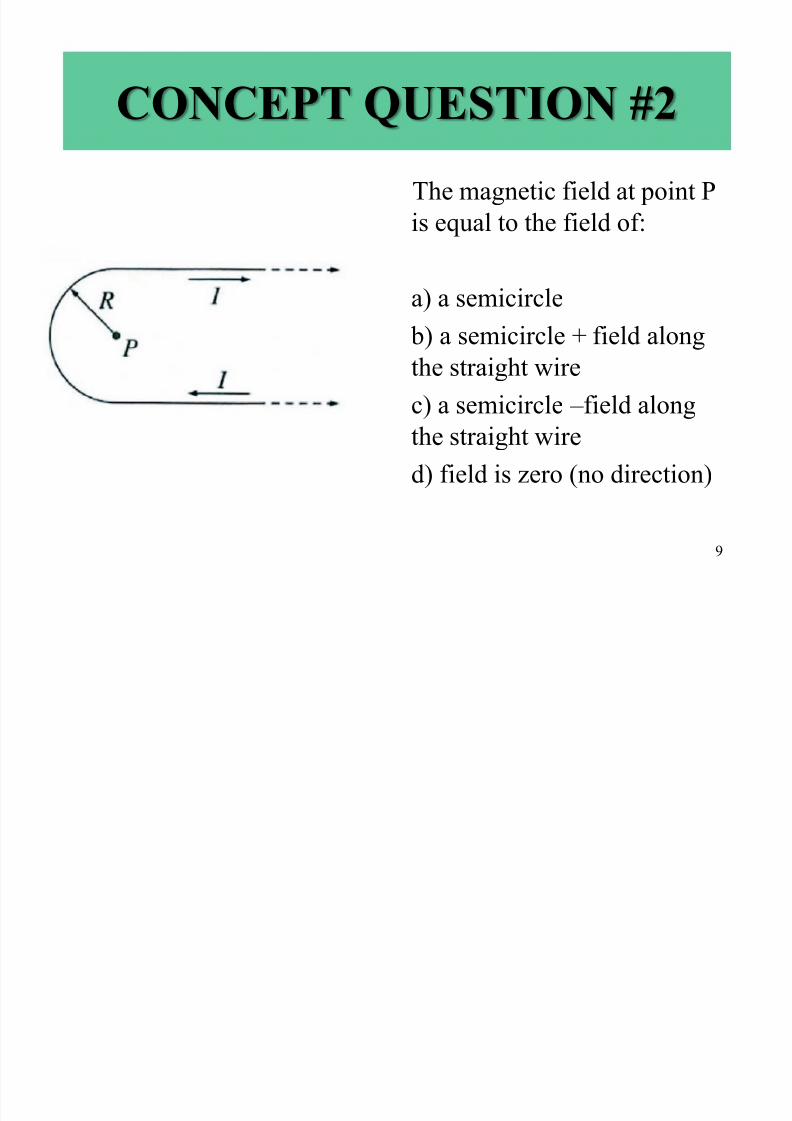
CONCEPT QUESTION #2

The magnetic field at point P

is equal to the field of:

a) a semicircle

b) a semicircle + field along

the straight wire

c) a semicircle – field alongthe straight wire

d) field is zero (no direction)

9



10

• Thus the direction of d H can be determined by the right-hand rule

[Figure 7.2(a)], or by the right-handed-screw rule [Figure 7.2(b)].

•

It is customary to represent the direction of the magnetic fieldintensity H (or current I ) by a small circle with a dot or cross sign

depending on whether H (or I ) is out of or into the page (Figure 7.3).

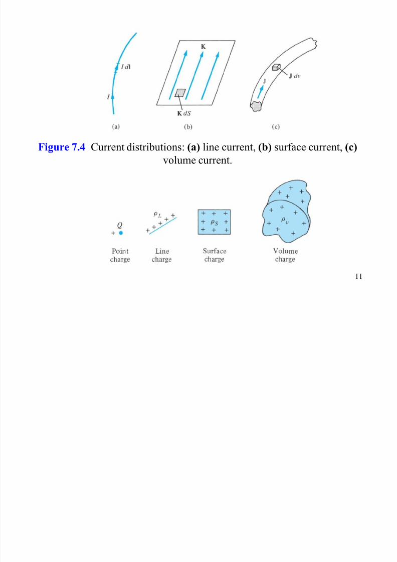
• Similar to charges, there are three different current distributions

which are: line current, surface current, and volume current (Figure7.4).

• If K defined as the surface current density (A/m) and J as the volume

current density (A/m2), the source elements are related as,

I d l = K d S = J dv (7.4)• Thus, the Biot-Savart's law becomes,

H = I d l a R (line current) (7.5)

4 R2



11

Figure 7.4 Current distributions: (a) line current, (b) surface current, (c)

volume current.



12

H = K d S a R (surface current) (7.6)

4 R2

H = J dv a R (volume current) (7.7)

4 R2

• As an example, to determine the field due to a straight current-

carrying filamentary conductor or finite length AB as in Figure 7.5.

• Assume that the conductor is along the z -axis, with its upper and

lower ends, respectively, subtending angles 1 and 2 at P , the pointat which H is to be determined.

• If the contribution d H at P due to an element d l at (0, 0, z),

d H = I d l R (7.8)

4 R3

But d l = dz a z and R = a - z a z , so



13

Figure 7.5



14

d l R = dz aΦ (7.9)

Hence,

H = I dz aΦ (7.10)

4[ 2 + z 2]3/2

Finally,

H = 1 (cos 2 – cos 1) aΦ (7.11)

4

• When the conductor is semi-infinite (with respect to P ) so that point A isnow at O (origin) while B is at (0, 0, ); 1 = 900, 2 = 00, and becomes

H = ( I / 4 ) aΦ (7.12)

• When the conductor is infinite in length (with respect to P ) so that point A

is at (0, 0,- ) while B is at (0, 0, ); 1 = 1800, 2 = 00, and becomes

H = ( I / 2 ) aΦ (7.13)

• A simple approach is to determine unit vector aΦ from,

aΦ = al a (7.14)

Where; al : unit vector along line current

a : unit vector along perpendicular line



15

Example 7.1

The conducting triangular loop in Figure 7.6 (a)carries a current of 10A. Find H at (0, 0, 5) due to

side 1 of the loop.



16

Solution:

Observe that 1, 2 and are assigned in the same manner as

in Figure 7.5 on which eq. 7.12 is based:

cos 1 = cos 90 = 0, , = 5

According to eq. 7.15 and , so

Hence,

= -59.1 a y mA/m

29

2cos 2

xaa z

aa

y z x aaaa

y

I aaH

0

29

2

54

10coscos

4121

aΦ = al a



17

Example 7.2

Find H at (-3, 4, 0) due to the current filamentshown in Figure 7.7 (a)



18

Solution:

Let H = H1 + H2 where H1 and H2 are the contributions to the

magnetic field intensity at P (-3, 4, 0) due to the portions of thefilament along x and z , respectively.

At P (-3, 4, 0), ρ = (9 + 16)1/2 = 5, 1 = 90, 2 = 0, and a is

obtained as a unit vector along the circular path through P on

plane z as in Figure 7.7(b).

The direction of a is determined using the right-handed-screw

rule or the right-hand rule. From the geometry in Fig. 7.7(b)

aH 122 coscos4

I

y x y x aaaaa5

3

5

4cossin



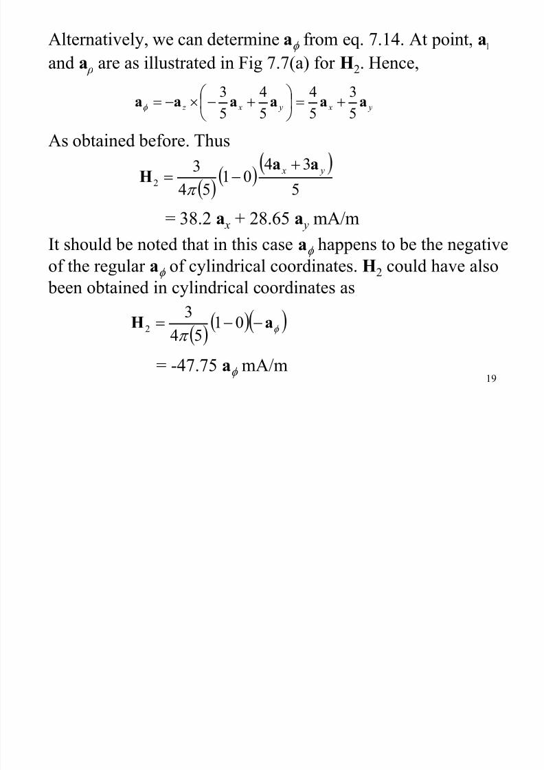
19

Alternatively, we can determine a from eq. 7.14. At point, al

and a ρ are as illustrated in Fig 7.7(a) for H2. Hence,

As obtained before. Thus

= 38.2 a x + 28.65 a y mA/m

It should be noted that in this case a happens to be the negative

of the regular a of cylindrical coordinates. H2 could have also

been obtained in cylindrical coordinates as

= -47.75 a mA/m

y x y x z aaaaaa53

54

54

53

5

3401

54

32

y x aaH

aH 01

54

32



20

Similarly, for H1 at P , ρ = 4, 1 = 0 = 3/5, and a = a z or a =a

lx a

ρ= a x x a y = a z . Hence,

= 23.88 a z mA/m

Thus

H = H1 + H2 = 38.2 a x + 28.65 a y + 23.88 a z mA/m

Or

H = -47.75 a + 23.88 a z mA/m

z aH

5

31

44

31



Brain Teaser

21

stand

5432 _ ?



22

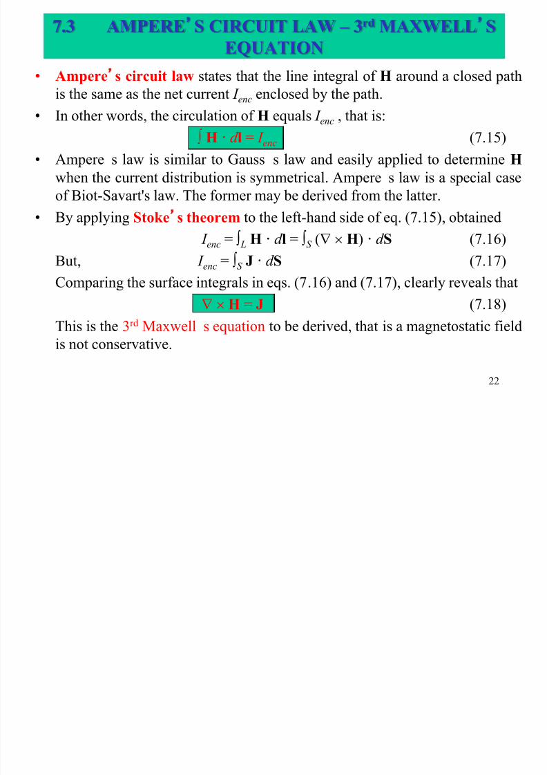
7.3 AMPERE’S CIRCUIT LAW – 3rd MAXWELL’S

EQUATION

• Ampere’s circuit law states that the line integral of H around a closed path

is the same as the net current I enc enclosed by the path.• In other words, the circulation of H equals I enc , that is:

H · d l = I enc (7.15)

• Ampere’s law is similar to Gauss’s law and easily applied to determine H

when the current distribution is symmetrical. Ampere’s law is a special case

of Biot-Savart's law. The former may be derived from the latter.

• By applying Stoke’s theorem to the left-hand side of eq. (7.15), obtained

I enc = L H · d l = S ( H) · d S (7.16)

But, I enc = S J · d S (7.17)

Comparing the surface integrals in eqs. (7.16) and (7.17), clearly reveals that H = J (7.18)

This is the 3rd Maxwell’s equation to be derived, that is a magnetostatic field

is not conservative.



23

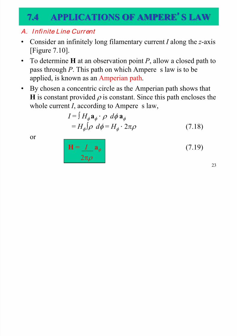
A. I nfi nite L ine Current

• Consider an infinitely long filamentary current I along the z -axis[Figure 7.10].

• To determine H at an observation point P , allow a closed path to

pass through P . This path on which Ampere’s law is to be

applied, is known as an Amperian path.

• By chosen a concentric circle as the Amperian path shows that

H is constant provided is constant. Since this path encloses the

whole current I , according to Ampere’s law,

I = H a · d a

= H d = H · 2 (7.18)

or

H = I a (7.19)

2

7.4 APPLICATIONS OF AMPERE’S LAW



24

Figure 7.10



25

B. I nf ini te Sheet of Current

• Consider an infinite current sheet z = 0 plane. If the sheet has a

uniform current density K = K y a y A/m as shown in Figure 7.11.

• Applying Ampere’s law to the rectangular closed path gives,

H · d l = I enc = K yb (7.20)

• To evaluate the integral H needs to regard the infinite sheet ascomprising of filaments; d H above or below the sheet due to a pair

of filamentary current can be found by using eqs. (7.13) and (7.14).

• As evident in Figure 7.11(b), the resultant d H has only an x-

component and H on one side of the sheet is the negative of that on

the other side.

H = ( I / 2 ) a (7.13)

aΦ = al a (7.14)



26

Figure 7.11



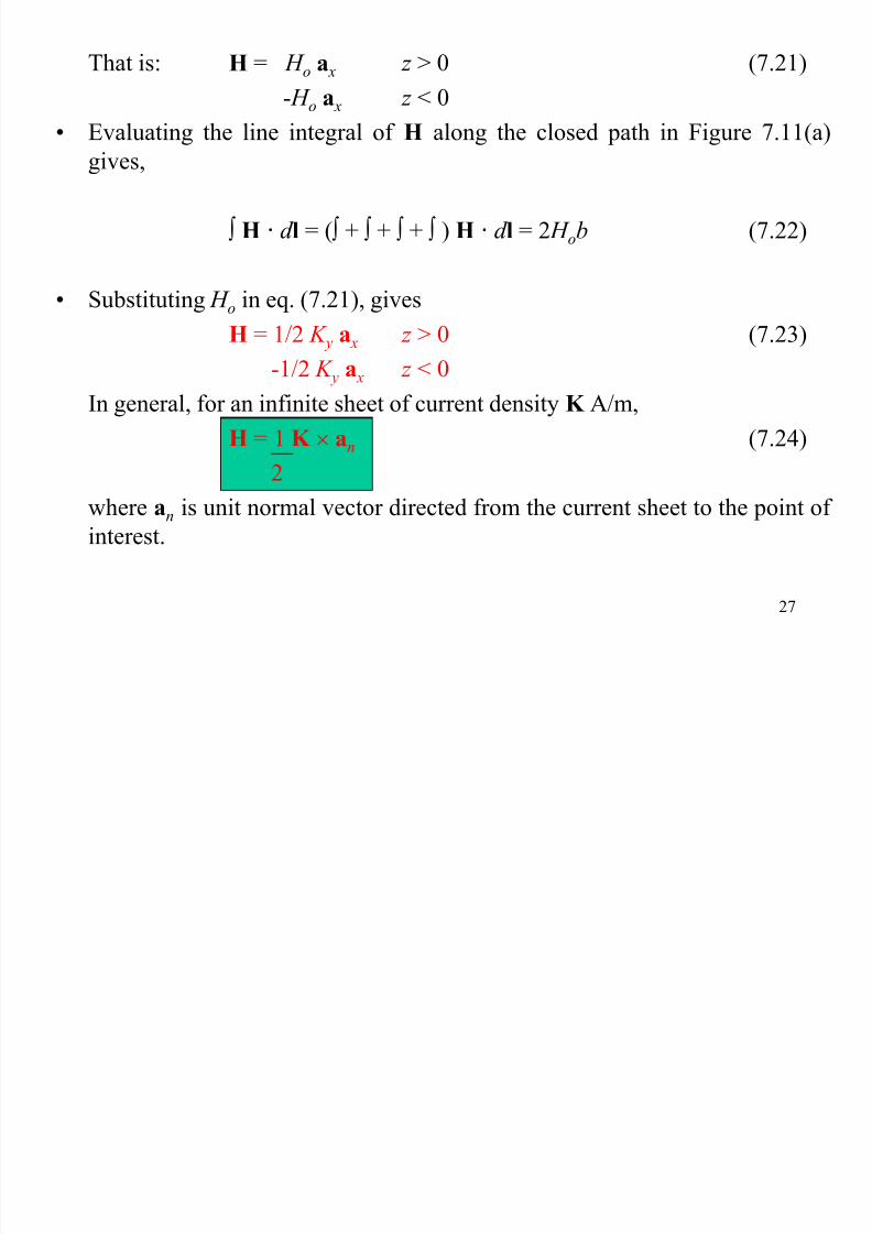
27

That is: H = H o a x z > 0 (7.21)

- H o a x z < 0

• Evaluating the line integral of H along the closed path in Figure 7.11(a)

gives,

H · d l = ( + + + ) H · d l = 2 H ob (7.22)

• Substituting H o in eq. (7.21), givesH = 1/2 K y a x z > 0 (7.23)

-1/2 K y a x z < 0

In general, for an infinite sheet of current density K A/m,

H = 1 K an (7.24)

2

where an is unit normal vector directed from the current sheet to the point of

interest.



28

C. I nf in itely Long Coaxial Transmission Line

• Consider an infinitely long transmission consisting of two concentric

cylinder having their axes along the z -axis [Figure 7.12].

• The inner conductor has radius a and carries current I , while the outer

conductor has inner radius b and the thickness t and carries return current - I .

Need to determined H everywhere, assuming that current is uniformly

distributed in both conductors.

•

Since the current distribution is symmetrical, apply Ampere’

s law along theAmperian path for each of the four possible regions: 0 a, a b,

b b + t , and b + t .

• For region 0 a, applied Ampere’s law to path L1 giving,

L1 H · d l = I enc = J · d S (7.25)

So that, J = I a z , d S = d d a z (7.26)

a2



29

Figure 7.12



30

I enc = J · d S = I d d = I 2 = I 2 (7.27)

a2 a2 a2

Hence eq. (7.26) becomes,

H dl = H 2 = I 2

/a2

or H = I

2a2

• For region a b, used path L2,

L2 H · d l = I enc = I

H 2 = I or H = I / 2 (7.28)

since the whole current I is enclosed by L2.

• For region b b + t , used path L3, getting

L3 H · d l = H · 2 = I enc (7.29)

where I enc = I + J · d S



31

• In this case J is the current density of the outer conductor and isalong - a z , that is,

J = - I a z

[(b + t)2 - b2]thus, I enc = I 1 - 2 - b2

t 2 + 2bt

Substituting this in eq. (7.29), we have,

H = I 1 - 2

- b2

(7.30)2 t 2 + 2bt

• For region b + t , used path L4, getting

H · d l = I - I = 0

or

H = 0 (7.31)

• List all the equations together – Refer to Eq. 6.29, Pg. 246



32

7.5 MAGNETIC FLUX DENSITY – 4rd MAXWELL’S

EQUATION

• Magnetic flux density B is similar to the electric flux density D. As D = oE

in free space, the B is related to the magnetic field intensity H according toB = oH (7.32)

where o is a constant known as the permeability of free space. Unit H/m

and has the value of,

o = 4 10-7 H/m (7.33)

• The magnetic flux through a surface S is given by,

= S B · d S (7.34)

where the magnetic flux is in webers (Wb) and the magnetic flux density B

is Wb/m2.

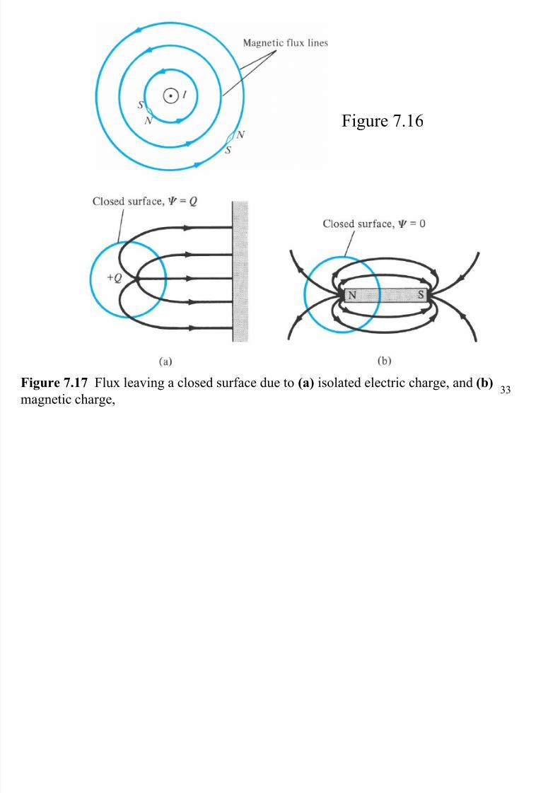
• A magnetic flux line is a path to which B is tangential at every point on the

line. For example, the magnetic flux lines due to a straight line long wire are

shown in Figure 7.16.

• The direction of B is taken as that indicated as “north” by the needle of the

magnetic compass.



33

Figure 7.16

Figure 7.17 Flux leaving a closed surface due to (a) isolated electric charge, and (b)

magnetic charge,



34

• Notice that each flux line is closed and has no beginning or end.

Though Figure 7.16 is for a straight, current-carrying conductor, it is

generally true that magnetic flux lines are closed and do not cross each

other regardless of the current distribution.• Thus it is possible to have an isolated electric charge as shown in Figure

7.17(a), which also reveals that electric flux lines are not necessarily

closed.

• Unlike electric flux lines, magnetic flux lines always close uponthemselves as in Figure 7.17(b). This is because it is not possible to

have isolated magnetic poles (or magnetic charges).

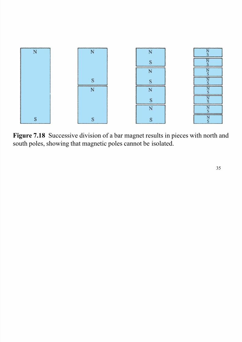
• For example, if desired to have an isolated magnetic pole by dividing a

magnetic bar successively into two, and ends up with pieces each

having north and south poles as illustrated in Figure 7.18.



35

Figure 7.18 Successive division of a bar magnet results in pieces with north and

south poles, showing that magnetic poles cannot be isolated.



36

• An isolated magnetic charge does not exist.

• Thus the total flux through a closed surface in a magnetic field must be

zero, that is,

B · d S = 0 (7.35)

• This equation is referred to as the law of conservative of magnetic

flux or Gauss ’ s law for magnetostatic field. Although the

magnetostatic field is not conservative, magnetic flux is conserved.

• By applying the divergence theorem to eq. (7.35), obtained,

S B · d S = v · B dv = 0

or · B = 0 (7.36)

• This equation is the fourth Maxwell’s equation to be derived where eq.

(7.35) or (7.36) shows that magnetostatic field have no sources or sinks.

Eq. (7.36) suggests that magnetic field lines are always continuous.



37

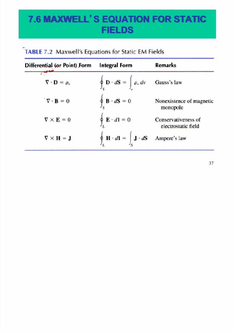
7.6 MAXWELL’S EQUATION FOR STATIC

FIELDS



38

7.7 MAGNETIC SCALAR & VECTOR POTENTIALS

• The magnetic potential could be scalar V m or vector A. Todefine V

mand A involves recalling two important identities:

(V ) = 0

· ( A) = 0

which must always hold for any scalar field V and vector field A.

• Definition of magnetic scalar potential V m (A) as related to H

according to,

H = - V m if J = 0 (7.37)

• Combining eqs. (7.37) and (7.18) gives,

J = H = (- V m) = 0 (7.38)

since V m must satisfy the condition in identity above, thus V m isonly defined in a region where J = 0. V m also satisfies Laplace'sequation, hence

2V m = 0 (J = 0) (7.39)



39

• Know that for a magnetostatic field, · B = 0, then can define the

vector magnetic potential A (Wb/m) such as

B = A (7.40)

• Just as defined, V = dQ

4 r

then can defined these equations,

A = o I d l (line current) (7.41)

4 R

A = oK dS (surface current) (7.42)

4 R

A = oJ dv (volume current) (7.43)

4 R

L

L

S

v



40

by substituting eq. (7.40) into eq. (7.34) and applying

Stoke’s theorem, obtained

= S B · d S =

S ( A) · d S =

L A · d l

or, = L A · d l (7.44)

• Thus the magnetic flux through a given area can be found by

using either eq. (7.34) or (7.44).

• Also, the magnetic field can be determined by using either V m or A. Where V m can be used only in a source-free region.



41

Example 7.7

Given the magnetic vector potential A = - 2/4 a z

Wb/m, calculate the total magnetic flux crossing the

surface = /2, 1 2 m, 0 z 5m.



42

Solution:

We can solve this problem in two different ways: using eq. 7.32

or eq. 7.51

Method 1:

, d S = d ρ d z a

Hence,

= 3.75 Wb

aaAB

2

z A

4

155

4

1

2

1 5

0

2

1

1

2

2 z dz d d

SB



43

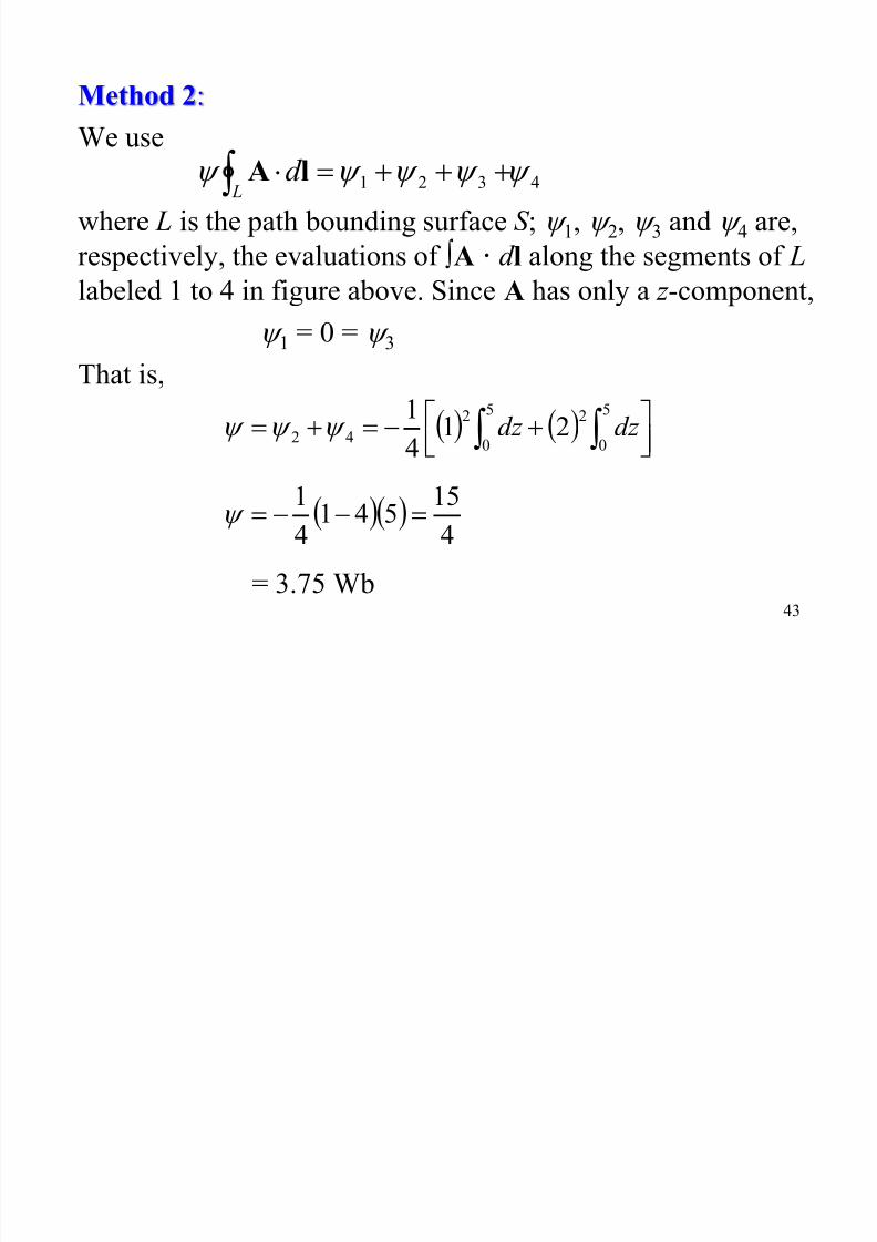
Method 2:

We use

where L is the path bounding surface S ; 1, 2, 3 and 4 are,

respectively, the evaluations of A · d l along the segments of L

labeled 1 to 4 in figure above. Since A has only a z -component,

1 = 0 = 3

That is,

= 3.75 Wb

4321 Ld lA

5

0

5

0

22

42 214

1dz dz

4

15541

4

1



44

• Both Biot-Savart's law and Ampere’s law may be derived by using the

concept of magnetic vector potential, which is

A = ( · A) - 2A (7.45)

• Thus the Biot-Savart's law becomes,

B = oI d l aR (7.46)

4 R 2

• Using the identity in eq. (7.45) with eq. (7.40), obtained

B = ( · A) - 2A (7.45)

on magnetostatic field, · A = 0. Upon replacing B with oH becomes,

2A = - o H or 2A = - oJ (7.47)

is called vector Poisson’s equation.

7.8 DERIVATION OF BIOT-SAVART’S LAW &

AMPERE’S LAW (from potential of vector A)



45

• For scalar Poisson’s equations, in coordinates Cartesian

may be decomposed into 3 scalar equations:

2 A x = - oJ x ;

2 Ay = - oJ y ;

2 Az = - oJ z (7.48)

• It can also be shown that Ampere’s circuit law is consistent

with our definition of the magnetic vector potential by using

the vector identity related to A.

Documents

Chapter 7 Magnetostatic