Chapter 7: Map projections - SFU.ca - Simon Fraser …hickin/Maps/Chapter 7.pdfChapter 7: Map projections 78 (c) Oblique orientation refers to any intermediate orientation and tangency

75

Chapter 7: Map projections

Introduction Large-scale field maps involve transferring information from a sensibly flat piece of land to a flat

map. Because we are representing the topography on the same type of mean surface, mapping is

achieved directly by down-scaling a real-world rectangular grid to a model rectangular grid. As the area to

be mapped increases, however, distortion begins to appear simply because the Earth's surface is not

planar but curved. Even on the 1:50 000 NTS sheets we have found that a single map area is sufficiently

large for the Earth's curvature to cause a small divergence of the rectangular UTM grid lines from the

lines of longitude.

On small-scale maps it simply is not possible to accurately represent on the planar surface of a

map the true geographic properties of the spherical surface of our Earth. Only a globe provides an

analogous distortion-free modeling surface; all world maps involve distortion of one sort or another. A

perfectly analogous problem is encountered if you try and lay flat on a table the intact skin of a peeled

orange! It is only possible if the skin is stretched or broken or in other ways distorted from its original

spherical shape.

The transfer of geographic information from the spherical Earth to a planar map sheet is

accomplished by the use of map projections; this chapter is concerned with their construction and

properties.

Types of Map Projection

Although the term 'projection' is used to describe the various transformations that enable us to

view the spherical surface of the earth on a planar map, only a few actually are true 'projections' in the

optical sense of the word. Indeed, there are two broad classes of "projections": true projections, and

those based on mathematical transformations.

True projections

These are formed by the projection of the earth's graticule of meridians and parallels on to some

sort of screen or projection surface. Thus it is useful to imagine the earth as a transparent globe, perhaps

made of clear glass, on which the meridians and parallels are painted as black lines. The position of the

light source may be inside or outside the globe and of course the screen or projection surface can vary in

shape as well.

Projection surfaces are of two general types: (a) a plane surface; and (b) developable surfaces.

(a) The plane surface is the simplest projection surface and provides the most direct link between

the global geography and the map. A plane can only touch the surface of a sphere at a single point of

tangency and for this one unique point there is no distortion of the spherical grid on the map. For all other


76

points, however, map distortion occurs and increases with distance from the point of tangency. Because

directions from the point of tangency are shown correctly on a plane surface, these projections are also

known as azimuthal projections. It is the type of projection surface usually used to map the polar regions

of the planet.

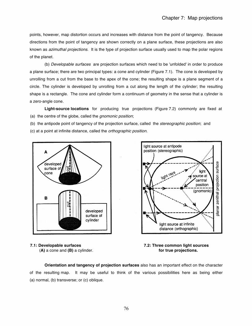
(b) Developable surfaces are projection surfaces which need to be 'unfolded' in order to produce

a plane surface; there are two principal types: a cone and cylinder (Figure 7.1). The cone is developed by

unrolling from a cut from the base to the apex of the cone; the resulting shape is a plane segment of a

circle. The cylinder is developed by unrolling from a cut along the length of the cylinder; the resulting

shape is a rectangle. The cone and cylinder form a continuum of geometry in the sense that a cylinder is

a zero-angle cone.

Light-source locations for producing true projections (Figure 7.2) commonly are fixed at

(a) the centre of the globe, called the gnomonic position;

(b) the antipode point of tangency of the projection surface, called the stereographic position; and

(c) at a point at infinite distance, called the orthographic position.

7.1: Developable surfaces 7.2: Three common light sources (A) a cone and (B) a cylinder. for true projections.

Orientation and tangency of projection surfaces also has an important effect on the character

of the resulting map. It may be useful to think of the various possibilities here as being either

(a) normal, (b) transverse; or (c) oblique.


77

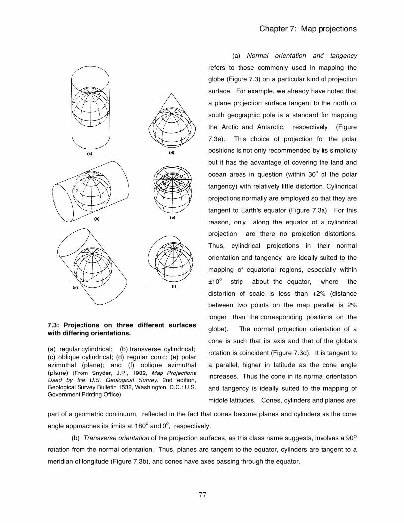
7.3: Projections on three different surfaces with differing orientations. (a) regular cylindrical; (b) transverse cylindrical; (c) oblique cylindrical; (d) regular conic; (e) polar azimuthal (plane); and (f) oblique azimuthal (plane) (From Snyder, J.P., 1982, Map Projections Used by the U.S. Geological Survey. 2nd edition, Geological Survey Bulletin 1532, Washington, D.C.: U.S. Government Printing Office).

(a) Normal orientation and tangency

refers to those commonly used in mapping the

globe (Figure 7.3) on a particular kind of projection

surface. For example, we already have noted that

a plane projection surface tangent to the north or

south geographic pole is a standard for mapping

the Arctic and Antarctic, respectively (Figure

7.3e). This choice of projection for the polar

positions is not only recommended by its simplicity

but it has the advantage of covering the land and

ocean areas in question (within 30o of the polar

tangency) with relatively little distortion. Cylindrical

projections normally are employed so that they are

tangent to Earth's equator (Figure 7.3a). For this

reason, only along the equator of a cylindrical

projection are there no projection distortions.

Thus, cylindrical projections in their normal

orientation and tangency are ideally suited to the

mapping of equatorial regions, especially within

±10o strip about the equator, where the

distortion of scale is less than +2% (distance

between two points on the map parallel is 2%

longer than the corresponding positions on the

globe). The normal projection orientation of a

cone is such that its axis and that of the globe's

rotation is coincident (Figure 7.3d). It is tangent to

a parallel, higher in latitude as the cone angle

increases. Thus the cone in its normal orientation

and tangency is ideally suited to the mapping of

middle latitudes. Cones, cylinders and planes are

part of a geometric continuum, reflected in the fact that cones become planes and cylinders as the cone

angle approaches its limits at 180o and 0o, respectively.

(b) Transverse orientation of the projection surfaces, as this class name suggests, involves a 90o

rotation from the normal orientation. Thus, planes are tangent to the equator, cylinders are tangent to a

meridian of longitude (Figure 7.3b), and cones have axes passing through the equator.


78

(c) Oblique orientation refers to any intermediate orientation and tangency of the projection

surface between the limiting classes of normal and transverse transformations (Figure 7.3c and f).

Mathematical projections

Not all 'projections' are true optical projections. Many are generated mathematically and the

character of these transformations often are difficult to visualize. The spherical graticule of the globe is

transformed in various ways to satisfy certain criteria and it will be easiest to examine this group of

projections in terms of the few examples below.

General properties of projections in relation to the globe

Because of its similarities to Earth, a sphere is a useful reference surface in any discussion of

map projections. On a sphere, features of the earth's surface - their shape, area, and distance and

directions between them - are shown correctly. The manner and degree to which these properties are

distorted can be evaluated by reference to the spherical graticule forming the parallels of latitude and

meridians of longitude (see Figure 1.11). It might be useful to remind ourselves of the properties of this

spherical grid system:

(a) Parallels of latitude measure an angle from Earth's centre in the polar plane, north and south

with respect to the equator (0o); thus the geographic north and south poles are at respective latitudes 90o

N and 90o S and the total latitudinal angular sweep from pole to pole is 180o.

(b) Parallels of latitude are indeed parallel, each with all others.

(c) Parallels of latitude are equally spaced; the polar circumference is approximately 40 008 km so that 1o of latitude corresponds with a spacing of

20 004km180o or 111.13 km on Earth's surface.

(d) Parallels of latitude are of unequal length. The longest parallel is the equator (40 076 km) and

others decline in length north and south to a limiting point at the poles as follows:

0o = 40 076 km 20o = 37 674 km 40o = 30 743 km 60o = 20 084 km 80o = 6 982 km 10o = 39 471 km 30o = 34 736 km 50o = 25 812 km 70o = 13 748 km 90o = 0 km

(e) Meridians of longitude measure an angle from Earth's centre in the equatorial plane, 180o east

and west with respect to the prime meridian (0o) through Greenwich, England; thus the total meridianal

angular sweep is a full circle of 360o.

(f) All meridians pass through both poles and are equal in length (40 008 km).

(g) Meridians are not parallel and meridian spacing varies from 0 km where meridians meet at the poles to a maximum at the equator. 1o of equatorial longitude corresponds to a spacing of

40 076km360o

or 111.32 km, while the corresponding spacing at intermediate latitudes of 20o, 40o, 60o, and 80o, for

example, is respectively 104.65 km, 85.40 km, 55.79 km, and 19.39 km.

(h) Parallels of latitude and meridians of longitude everywhere cross at right angles.


79

An ideal map projection retains all these graticule characteristics through the translation to the

map. But the ideal map projection can never be achieved and if a projection is designed to guarantee a

particular characteristic as true, others on it necessarily will be distorted. As a result map projections will

possess certain specific qualities of the globe but never all of them. In particular, map projections may be

evaluated in terms of how well they preserve several global spatial dimensions: shape, area, distance,

and direction.

Conformality is the term used to describe the property of correct shape retention on a map;

such maps are said to be orthomorphic. The importance of conformality is that map features can be

recognized by their distinctive shapes. If shapes are correct then directions must also be correct. It is

necessary that, on all conformal maps, lines of latitude and longitude must cross at right angles and that

the scale must be the same in all directions at any given point, just as is the case on the globe. Obviously

the term conformal is somewhat misleading because there can be no such thing as a truly conformal map

of the globe. But true shapes of small features may be retained on a conformal map and the term is

useful to denote this specific quality.

Equivalence refers to the retention of correct relative global areas on a map. Although it is

possible to achieve equivalence in global map, such a projection always creates severe distortions in

shape of the lands involved. To retain equivalence, any scale changes that occur in one direction must

be offset by appropriate changes in the normal direction. Such projections obviously are important for

maps depicting accurate relative areas.

Distance relationships on a map can be correctly depicted only if the length of a straight line

between two points on the map projection represents the great circle distance between the same two

points on the globe. It is only possible to depict correct distances on a map from one, or at most, two

points. The azimuthal equidistant projection achieves this for all lines from the polar position (but for no

others).

Direction is correctly retained on a projection when a straight line drawn between two points on

the map shows the correct azimuth of the line; the azimuth is defined by the angle formed at the starting

point of the straight line. In other words, a projection depicting true direction must show the great circle

routes between points as straight lines. This is one of the properties of a gnomonic projection. Note that

true direction or azimuth does not mean true bearing, an important distinction we will discuss later in the

context of describing Mercator's projection.

Some commonly used map projections

Rather than attempt a comprehensive cataloguing of the many different types of map projections

in use, here we will simply examine the character of several examples which are either commonly used

map projections, or have particularly instructive properties. Exhaustive treatments are available, however,

and the reader interested in exploring this topic further is referred to the Chapter 7 reference list at the


80

end of the manual.

The projections considered here illustrate well the general problem of transforming a spherical

surface to a plane. Insights gained from evaluating these examples will help in assessing other map

projections we might encounter in the future. Our examples constitute four groups, (a) cylindrical-type

projections, (b) a compromise projection (Mollweide's), (c) zenithal projections, and (d) conical-type

projections:

(a) Cylindrical-type projections

1. Perspective cylindrical projection

2. Plate carrée (or simple cylindrical or

cylindrical equidistant projection

3. Cylindrical equal area projection

4. Mercator's projection (cylindrical orthomorphic)

5. Sinusoidal projection

6. Interrupted sinusoidal

(b) A compromise projection

7. Mollweide's projection

(c) Zenithal projections

8. Gnomonic projection

9. Stereographic projection

10. Orthographic projection

11. Zenithal equidistant projection

12. Zenithal equal-area projection

(d) Conical-type projections

13. Perspective conic projection

14. Simple conic projection: one standard parallel

15. Bonne's projection

16. Conic projection with two standard parallels

17. Polyconic projection

(a) Cylindrical-type projections

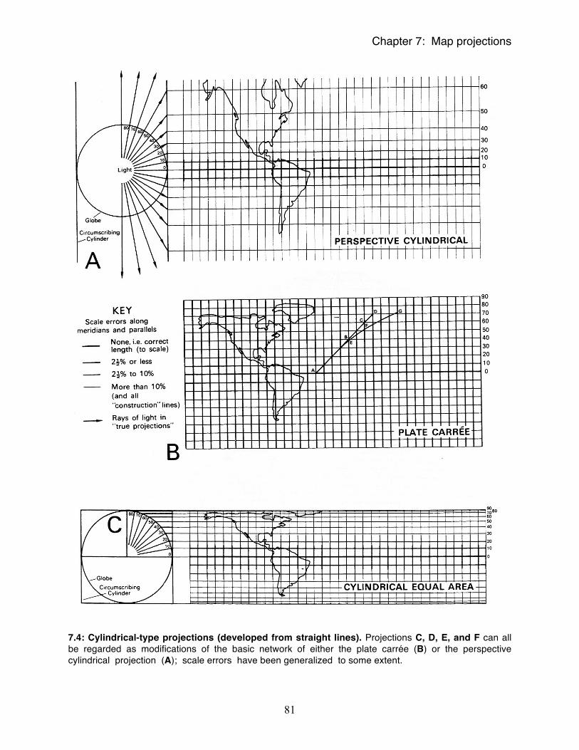
The perspective cylindrical projection (Figure 7.4A) can be thought of as the basic model from

which all the projections in the first group are derived. It is a true projection formed by projecting a globe

from its centre onto a circumscribing cylinder. Beyond providing a basis for modification, however, it is of

little practical use because of the obviously extreme scale-distortion at high latitudes; clearly the parallel

length and meridian spacing should decline towards the poles. The only redeeming feature of this

projection is that, within 10o of the equator, scale distortion is less than a few per cent. Because it can

be readily improved, other derivative projections are distinctly superior.

The plate carrée (or simple cylindrical or cylindrical equidistant) projection is not a true

projection but we can think of it as a cylindrical-type projection. It is a rectilinear graticule in which the

meridians are true length and parallels all equal the length of the equator and are correctly spaced as on

the globe (Figure 7.4B). As in the case of all cylindrical-type projections, however, because the meridian

spacing does not decline toward the poles, the polar regions consequently are highly distorted.

Nevertheless, although neither shape nor area can be correctly depicted on this projection, within a 5o

strip on either side of the equator, exaggeration along the parallels is less than +0.38%.


81

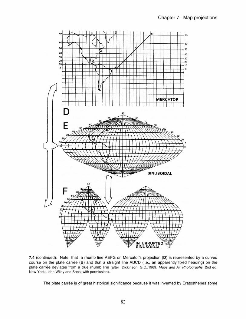
7.4: Cylindrical-type projections (developed from straight lines). Projections C, D, E, and F can all be regarded as modifications of the basic network of either the plate carrée (B) or the perspective cylindrical projection (A); scale errors have been generalized to some extent.


82

7.4 (continued): Note that a rhumb line AEFG on Mercator's projection (D) is represented by a curved course on the plate carrée (B) and that a straight line ABCD (i.e., an apparently fixed heading) on the plate carrée deviates from a true rhumb line (after Dickinson, G.C.,1969, Maps and Air Photographs. 2nd ed. New York: John Wiley and Sons; with permission).

The plate carrée is of great historical significance because it was invented by Eratosthenes some


83

two thousand years ago and has been used as a map base at various times since then until quite

recently. For example, it was used for the early editions of the Ordnance Survey maps of England and

Wales.

The cylindrical equal-area projection is a true projection in which a light from a source in the

orthographic position (at infinite distance) is projected onto a cylindrical surface in the normal orientation

and tangency (Figure 7.4C). Alternatively, we can think of the cylindrical equal-area projection as a

perspective cylindrical (or plate carrée) projection in which the spacing of parallels has been adjusted so

that relative areas are shown correctly as they are on the globe. As the parallels are stretched beyond

their true length toward the poles on this rectilinear graticule, the parallel spacing must be compressed in

compensation in order to preserve equal areas. Thus, the cost of obtaining equality of area on this

projection is gross scale distortion in high latitudes. In fact it turns out that there are better solutions to

this equal-area problem than that offered by the cylindrical equal-area projection and it is little used in

modern cartography.

Mercator's projection (cylindrical orthomorphic) probably has been and remains the most widely

used (and abused) map projection during the last 400 years (Figure 7.4D). The Flemish geographer and

mathematician Gerardus Mercator (1512-1594) designed his projection in 1569 as a navigational aid for

sailors. He wanted a map on which a compass heading or line of constant bearing (rhumb line) would

appear as a straight line. This property would allow navigators to transfer compass headings directly to

the map and to directly measure course headings between points shown on the map. The Mercator

projection, like the other projections in this group, is a derivative of the perspective cylindrical or plate

carrée projections. Like the plate carrée it is based on a rectilinear graticule in which parallels are drawn

the same length as the equator throughout and meridian spacing corresponds to that on the equator. In

order to satisfy this particular navigational requirement, however, the parallel spacing (meridian length)

increases away from the equator at the same rate as the parallels lengthen compared with their true

length on the globe. Mercator's pre-calculus solution to this problem of continuous change was only

approximate but it was sufficiently accurate to be of great practical use to mariners.

The distinction between great circles and rhumb lines is important to appreciating the character

of Mercator's projection. If you trace out the shortest line between two points on the surface of the globe

you have traced a so-called great circle route. It is a segment of a circle whose centre is the centre of

the globe. For example, consider the great circle route between Vancouver, British Columbia and London

England. Because this is the shortest distance between these two points it is the non-stop route followed

by commercial airlines. Such a flight leaves Vancouver at a true northeast bearing (about 45o) but

approaches London on a southeast heading (about 135o). Midway in the flight, over Baffin Island, the

aircraft would have been flying parallel to the Arctic Circle (66.6oN) on a true east-west bearing of 90o. In

other words, because the great circle route diagonally crosses the spherical graticule, the bearing the

aircraft follows (as measured by an onboard magnetic compass) in order to keep to the great circle route,


84

is constantly changing.

The initial bearing from one point to another (45o at Vancouver in our example) is known as an

azimuth. It will be clear that flying a course set at the azimuth of 45o from Vancouver will not get our

aircraft to London! Such a line of constant bearing is known as a rhumb line. A 45o rhumb line from

Vancouver would take us on a curved course, spiraling in to the North Pole!

The problem facing Mercator was to produce a map which would show a straight line between

any two points as a rhumb line. The great utility of such a map is that a sailor could draw a straight line

between his planned point of departure and his destination and measure directly the compass heading he

would need to follow in order to successfully complete his journey. On Mercator's projection an azimuth

lies on a rhumb line. Since rhumb lines are not great circle routes (except for the special cases of a route

exactly on the equator or exactly on a meridian), it follows that a rhumb line course plotted on Mercator's

projection is not the shortest route. Conversely, great circle routes plotted on Mercator's projection

appear as curved lines. For example, a straight line between Vancouver and London on Mercator's

projection is an approximately east-west (90o) rhumb line which takes us on a southerly course over

Winnipeg and Newfoundland, and is about 20 per cent longer than the great circle route over Greenland.

But Mercator made no claim for economy; rather he claimed, 'a straight line between two points on

Mercator's projection is a rhumb line and if you keep your compass fixed to the rhumb line azimuth you

will reach your destination'. A navigator wanting both economy of travel and ease of navigation must use

two map projections. First, the route must be plotted on a gnomonic projection on which all straight lines

are great circle routes (but not rhumb lines). This route must then be transferred to Mercator's projection

where it will plot as a curved line. This arc can be broken up into a series of connected straight chords or

legs and thus each leg is a rhumb line yielding a compass heading. By sailing along this series of rhumb

lines a navigator can approximate the shortest route.

Scale distortion on Mercator's projection is very severe at high latitudes but quite tolerable (less

than +1.5%) within 10o of the equator. Above 60o latitude scale errors exceed +100% and become

infinite at the poles; we are all familiar with the typical school atlas showing Greenland as large as South

America when in fact it is only about one tenth of that continent's area! The alternative name for

Mercator's projection, the cylindrical orthomorphic projection, recognizes that it fulfills the property of

orthomorphism so that shapes over very small areas therefore are shown correctly.

Given its intended specialized navigational use, it is rather surprising how widely Mercator's

projection has been used as a basis for world maps. No doubt part of the explanation lies in the fact that

for many years in many places navigational charts were the most readily available maps, and indeed the

only ones available, and the inertia of convention has helped to keep it in use. In its transverse form it is

of course the projection (UTM) used here in Canada for the NTS.

The sinusoidal projection, also known as the Sanson-Flamsteed projection, is derived directly

from the plate carrée by adjusting the equatorial length of parallels, and therefore the spacing of the


85

meridians, so that they are equal to their true values for the globe. The result is a rather aesthetically

displeasing ellipsoidal outline pinched to a peak at both poles (Figure 7.4E). Nevertheless, it has the

virtue of a central region of minimal distortion rather than an equatorial strip as in the case of the plate

carrée, for example. As we move away from the equator and central meridian of this projection, however,

the graticule intersections increasingly skew from 90o so that in the peripheral areas shapes are highly

distorted. Still, compared with the perspective cylindrical projection, plate carrée, or Mercator's projection,

high latitude shapes and areas are far less distorted. In fact, the sinusoidal projection retains the property

of equivalence over the entire projection. This property follows from the theorem showing that

parallelograms with similar bases drawn between the same parallel lines are equal in area regardless of

shape. As an equal-area projection the sinusoidal projection is better than a cylindrical equal-area

projection which has extreme shape distortion at high latitudes.

A solution to the shape-distortion problem on the sinusoidal and certain other projections is to

interrupt the graticule along selected meridians. An interrupted version of the sinusoidal projection is

shown in Figure 7.4F. Here several central meridians of low distortion are employed along with graticule

breaks so that the overall shape distortion is reduced. But the result clearly is rather odd! Now we have a

map which appears to have been torn into strips and furthermore it cannot be reformed to an

uninterrupted version by cutting and pasting; adjoining sheets do not match well without boundary

distortion. Nevertheless, if we are just interested in seeing well-shaped equal-area continental areas on

the one projection, interruption can be confined to the oceans so that information loss and distortion is

minimal. Certainly you will find examples of interrupted projections in most world atlases.

(b) A compromise projection

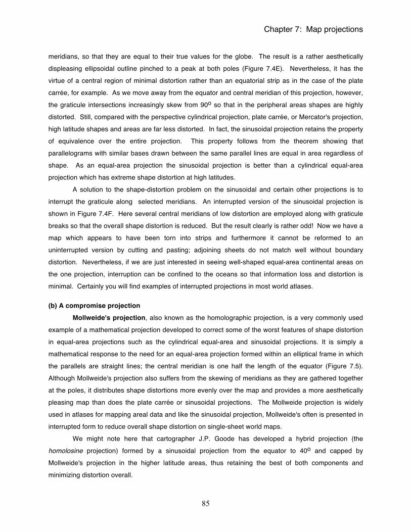
Mollweide's projection, also known as the homolographic projection, is a very commonly used

example of a mathematical projection developed to correct some of the worst features of shape distortion

in equal-area projections such as the cylindrical equal-area and sinusoidal projections. It is simply a

mathematical response to the need for an equal-area projection formed within an elliptical frame in which

the parallels are straight lines; the central meridian is one half the length of the equator (Figure 7.5).

Although Mollweide's projection also suffers from the skewing of meridians as they are gathered together

at the poles, it distributes shape distortions more evenly over the map and provides a more aesthetically

pleasing map than does the plate carrée or sinusoidal projections. The Mollweide projection is widely

used in atlases for mapping areal data and like the sinusoidal projection, Mollweide's often is presented in

interrupted form to reduce overall shape distortion on single-sheet world maps.

We might note here that cartographer J.P. Goode has developed a hybrid projection (the

homolosine projection) formed by a sinusoidal projection from the equator to 40o and capped by

Mollweide's projection in the higher latitude areas, thus retaining the best of both components and

minimizing distortion overall.


86

7.5: Mollweide's projection (after Dickinson, G.C.,1969, Maps and Air Photographs. 2nd ed. New York: John Wiley and Sons; with permission).

(c) Zenithal projections

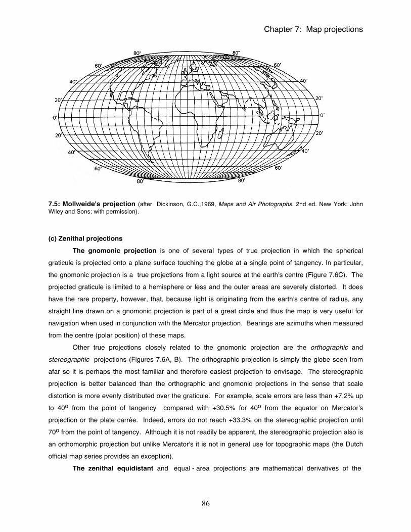
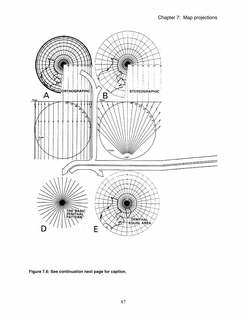
The gnomonic projection is one of several types of true projection in which the spherical

graticule is projected onto a plane surface touching the globe at a single point of tangency. In particular,

the gnomonic projection is a true projections from a light source at the earth's centre (Figure 7.6C). The

projected graticule is limited to a hemisphere or less and the outer areas are severely distorted. It does

have the rare property, however, that, because light is originating from the earth's centre of radius, any

straight line drawn on a gnomonic projection is part of a great circle and thus the map is very useful for

navigation when used in conjunction with the Mercator projection. Bearings are azimuths when measured

from the centre (polar position) of these maps.

Other true projections closely related to the gnomonic projection are the orthographic and

stereographic projections (Figures 7.6A, B). The orthographic projection is simply the globe seen from

afar so it is perhaps the most familiar and therefore easiest projection to envisage. The stereographic

projection is better balanced than the orthographic and gnomonic projections in the sense that scale

distortion is more evenly distributed over the graticule. For example, scale errors are less than +7.2% up

to 40o from the point of tangency compared with +30.5% for 40o from the equator on Mercator's

projection or the plate carrée. Indeed, errors do not reach +33.3% on the stereographic projection until

70o from the point of tangency. Although it is not readily be apparent, the stereographic projection also is

an orthomorphic projection but unlike Mercator's it is not in general use for topographic maps (the Dutch

official map series provides an exception).

The zenithal equidistant and equal - area projections are mathematical derivatives of the


87

Figure 7.6: See continuation next page for caption.


88

7.6: Zenithal projections. In the orthographic, stereographic, and gnomonic projections, a quarter of the graticule has been omitted to reveal the construction details (after Dickinson, G.C.,1969, Maps and Air Photographs. 2nd ed. New York: John Wiley and Sons; with permission).


89

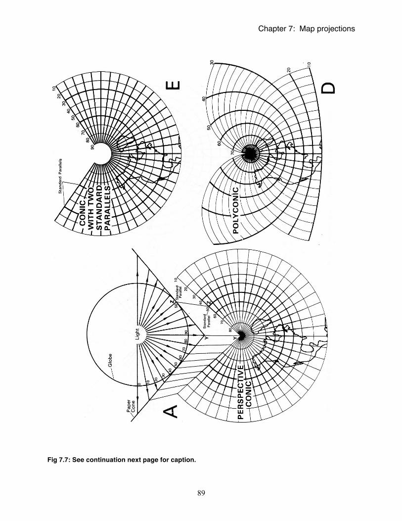
Fig 7.7: See continuation next page for caption.


90


91

orthographic-stereographic-gnomonic family of true projections (Figures 7.6 D, E, F). In its conventional

polar tangency the basic zenithal projection consists of straight meridians radiating from the pole which

intersect concentric parallels at right angles. In the zenithal equidistant projection the parallel spacing is

modified to show true distance along the meridians (but not in any other direction). The zenithal

projections are very good for depicting polar regions (even up to 45o scale distortions are less than about

+10%) and in their transverse or oblique forms they are usefully applied in other areas as well.

The zenithal equal-area projection is constructed by adjusting the spacing of parallels of the

basic zenithal projection so that they enclose on the map the same area as they do on the globe, thus

retaining the property of equivalence Figure 7.6E). It turns out that shape distortion is also minimal (less

than about +10%) within 50o of the pole as well.

As in all zenithal projections, directions from the centre of this projection are shown correctly as

azimuths of great circles. Zenithal projections are not widely used in topographic mapping, however,

because the conicals do an even better job of portraying small areas.

(d) Conical-type projections

The perspective conic projection (Figure 7.7) is the basic form of the final group of projections

to be considered here: those constructed on a conical surface. Although only one cylinder will fit the

globe, and a flat projection surface has fixed geometry, any number of different cones can rest on the

globe, from wide-angle types touching near the poles to low-angle cones touching near the equator.

Indeed, as we noted earlier the plane and cylinder can be thought of as limiting cones. The cone angle is

selected so that the circular contact between the cone and the globe best suits the area being mapped.

For example, the projections shown in Figure 7.7 make contact at 50o N because this tangency suits

maps of North America. In the normal orientation this line of tangency defines the standard parallel of

the projection.

As with cylindrical projections, the true or perspective conic projection is of little practical use but

it does provide a basic model for modification. The perspective conic projection has a standard parallel

shown at its correct length as an arc whose radius is the slant height of the cone at that point. Other

parallels are arcs of concentric circles; meridians are straight lines radiating from the centre of these

circles through points correctly spaced along the standard parallel. True distances along the parallels are

exaggerated away from the standard parallel (i.e., in both radial directions). Parallels and meridians

intersect at right angles, however, so we might expect minimal shape distortion.

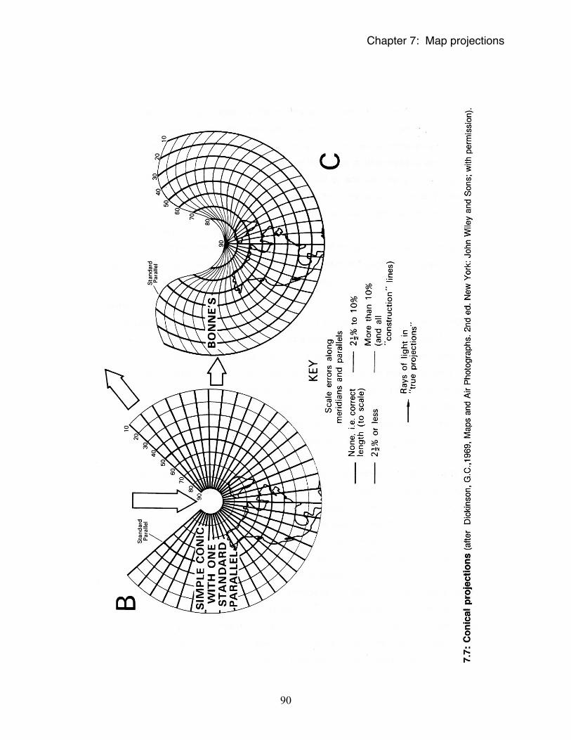
The simple conic projection with one standard parallel is a mathematical projection derived

from the perspective conic (Figure 7.6B). In this case, parallels are spaced at their true distance along

the meridians and the pole becomes a small arc rather than a point. As with the perspective conic

projection scale is exaggerated along all parallels other than the standard. Scale errors and thus

distortions in areas and shape are very small in a narrow band about the standard parallel.


92

Bonne's projection is a derivative of the simple conic with one standard parallel (Figure 7.6C).

It has been modified to remove the exaggeration of scale along the parallels by redrawing them at their

correct length. In consequence, meridians become curved lines and no longer intersect parallels at right

angles. Furthermore, meridians have been slightly stretched to longer than actual length. Nevertheless,

in spite of these shape distortions, Bonne's projection is an equal area projection and shapes and errors

are reasonably controlled about the central meridian. The projection is widely used in topographic

surveys and in atlas presentations.

The conic projection with two standard parallels, although essentially a mathematical

construct, can be envisaged as a derivative of the perspective conic. We can think of it as a spherical

graticule projected onto a cone which, instead of touching the globe at a point of tangency, intersects the

global surface at two parallels. These two standard parallels are then adjusted so that they are correctly

spaced as on the globe. Meridians are correctly spaced along the arcs of the two standard parallels and

radiate from the centre of the arcs. Other parallels are correctly spaced arcs concentric to the standard

parallels. The resulting graticule (Figure 7.6E) has properties similar to those of the simple conic

projection with one standard parallel except that errors are more evenly distributed across the map. Scale

is correct along all meridians and along both standard parallels (slightly too small between them and too

large along parallels outside the standards). Errors are quite small over large areas; for example, the

whole of U.S.A. can be mapped with less than 2% scale error.

The polyconic projection provides a means of extending the coverage of the conic projection

beyond a single hemisphere. The simple conic with one standard parallel set to accurately portray the

mid-latitudes of one hemisphere necessarily will produce a severely distorted and unacceptable view of

the other hemisphere. Employment of a second standard parallel can take our projection domain

somewhat beyond the equator with less overall distortion but the cost is increased specific distortion in

the polar region as well as in the mid latitudes, compared with that associated with a simple conic with a

standard parallel tangent in these regions. The polyconic projection is the logical extension of the error

distributing feature of the conic projection with two standard parallels. If two standard parallels generally

are better than one, then why not employ three or ten or one hundred? Well, obviously a single

cone cannot intersect the surface of a globe more than twice (to yield two standard parallels) but we can

solve this problem by using more than one cone. Indeed, in the polyconic projection every parallel is a

standard parallel and although it is a mathematical projection it can be conceived as being derived from

an infinite number of cones. Because the cone angle changes for each of these standard parallels they

are no longer concentric but they are spaced correctly along a central meridian and the meridians also are

correctly spaced along the parallels (Figure 7.7D). North-south scale errors increase rapidly away from

the central meridian so that the projection is of little use as a global map in the form shown in Figure 7.7D.

It is widely used in its interrupted form, however, with pole to pole mapping restricted to narrow strips

centred on the central meridian. For example, it is projection used in the International 1:1 000 000 map of


93

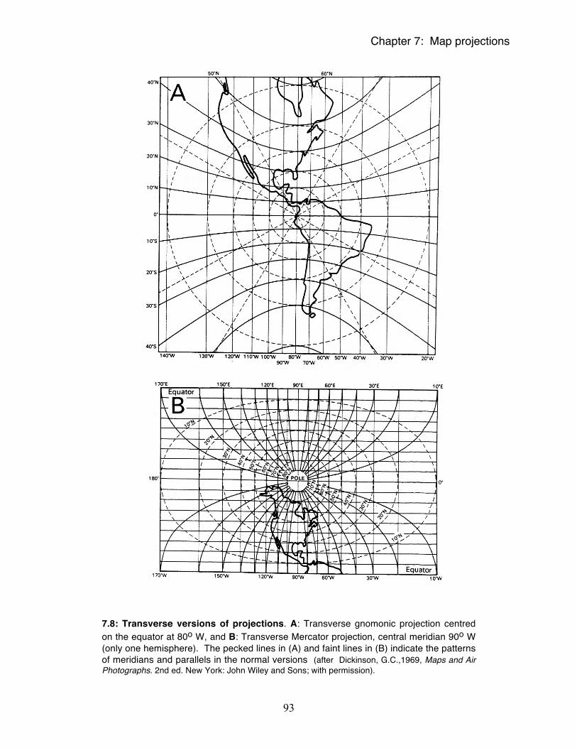
7.8: Transverse versions of projections. A: Transverse gnomonic projection centred on the equator at 80o W, and B: Transverse Mercator projection, central meridian 90o W (only one hemisphere). The pecked lines in (A) and faint lines in (B) indicate the patterns of meridians and parallels in the normal versions (after Dickinson, G.C.,1969, Maps and Air Photographs. 2nd ed. New York: John Wiley and Sons; with permission).


94

the world and in the maps of the United States Geological Survey.

Each of the above projections has been described in terms of its normal orientation and tangency

but of course every one can be rotated to any number of oblique positions or to a full transverse

orientation. These rotated projections often result in an unfamiliar pattern of parallels and meridians but

the properties of scale distortion of the projections are exactly the same as those in the normal

orientation. Figure 7.8 shows the graticule for the transverse Mercator projection (in this case, centred on

meridian 90oW), the basis of the National Topographic Series (NTS) here in Canada.

Choosing and Using Map Projections

Obviously care must be exercised in selecting projections for mapping. If comparative areal data

such as crop acreage are being shown, some type of equal-area projection should be employed. If

accurately depicting distances is more important, as it might be on a travel map, for example, then an

equidistant projection should be adopted. Navigation dictates the use of the gnomonic and Mercator's

projections, and so on.

Cartographic abuses are common and include deliberate exaggeration of areas for political and

other purposes. For example, it was common for the old British Empire to be shown on Mercator's

projection because it exaggerated the spatial importance of high latitude possessions such as Canada.

Similarly, opponents of Russia and the USSR could point to that country's menacing and dominating areal

presence with respect to lower latitude countries by selecting the 'right' projection.

Clearly the projection adopted must fit the purpose of the map and an important lesson of this

chapter is that many options are available and selecting an appropriate projection requires the exercise of

judgment. It also is fair to say that, although there usually is no one right solution to many mapping

problems, there are some reasonably unequivocally wrong solutions to certain others.

Documents

Chapter 7: Map projections - SFU.ca - Simon Fraser …hickin/Maps/Chapter 7.pdfChapter 7: Map projections 78 (c) Oblique orientation refers to any intermediate orientation and tangency