Embed Size (px)
Citation preview

DATABASESYSTEMSGROUP
Knowledge Discovery in Databases I: Numerical Prediction 1
Knowledge Discovery in DatabasesSS 2016
Lecture: Prof. Dr. Thomas Seidl
Tutorials: Julian Busch, Evgeniy Faerman,
Florian Richter, Klaus Schmid
Ludwig-Maximilians-Universität MünchenInstitut für InformatikLehr- und Forschungseinheit für Datenbanksysteme
Chapter 7: Numerical Prediction
© for the original version: Jörg Sander and Martin Ester, Jiawei Han and Micheline Kamber

DATABASESYSTEMSGROUP
Chapter 7: Numerical Prediction
1) Introduction
– Numerical Prediction problem, linear and nonlinear
regression, evaluation measures
2) Piecewise Linear Numerical Prediction Models
– Regression Trees, axis parallel splits, oblique splits
– Hinging Hyperplane Models
3) Bias-Variance Problem
– Regularization , Ensemble methods
Numerical Prediction 2

DATABASESYSTEMSGROUP
Numerical Prediction
• Related problem to classification: numerical prediction
– Determine the numerical value of an object
– Method: e.g., regression analysis
– Example: prediction of flight delays
• Numerical prediction is different from classification
– Classification refers to predict categorical class label
– Numerical prediction models continuous-valued functions
• Numerical prediction is similar to classification
– First, construct a model
– Second, use model to predict unknown value
• Major method for numerical prediction is regression
– Linear and multiple regression
– Non-linear regression
Classification Introduction 3
Windspeed
Delay offlight
query
predictedvalue
DATABASESYSTEMSGROUP
Examples
Housing values in suburbs of Boston
• Inputs
– number of rooms
– Median value of houses in the
neighborhood
– Weighted distance to five Boston
employment centers
– Nitric oxides concentration
– Crime rate per capita
– …
• Goal: compute a model of the housing values, which can be used to predict the price for a house in that area
Numerical Prediction Introduction 4

DATABASESYSTEMSGROUP
Examples
• Control engineering:
– Control the inputs of a system in
order to lead the outputs to a given
reference value
– Required: a model of the process
Numerical Prediction Introduction 5
measured outputs
optimizationprocess model
Process
Controller
Inputs(manipulated variables)
Diesel engineWind turbine

DATABASESYSTEMSGROUP
Examples
• Fuel injection process:
– database of spray images
– Inputs: settings in the pressure chamber
– Outputs: spray features, e.g., penetration
depth, spray width, spray area
Numerical Prediction Introduction 6
compute a model which predicts the spray features, for input settings which have not been measured

DATABASESYSTEMSGROUP
Numerical Prediction
• Given: a set of observations
• Compute: a generalized model of the data which enables the prediction of the output as a continuous value
• Quality measures:
– Accuracy of the model
– Compactness of the model
– Interpretability of the model
– Runtime efficiency (training, prediction)
Numerical Prediction Introduction 7
Numerical
Prediction
model
Inputs
(predictors)
Outputs
(responses)

DATABASESYSTEMSGROUP
Linear Regression
• Given a set of 𝑁 observations with inputs of the form 𝐱 = [𝑥1, … , 𝑥𝑑] and
outputs 𝑦 ∈ ℝ
• Approach: minimize the Sum of Squared Errors (SSE)
• Numerical Prediction: describe the outputs 𝑦 as a linear equation of the
inputs
• Train the parameters 𝜷 = [𝛽0 𝛽1 …𝛽𝑑]:
𝑖=1
𝑁
𝑦𝑖 − 𝑓 𝐱𝑖2→ 𝑚𝑖𝑛
Numerical Prediction Introduction 8
𝑑 = 1: 𝑦 = 0,5645 ⋅ 𝐱 + 1,2274
0
1
2
3
4
0 1 2 3 4𝑥
𝑦
ො𝑦 = 𝑓 𝐱 = 𝛽0 + 𝛽1 ⋅ 𝑥1 + …+ 𝛽𝑑 ⋅ 𝑥𝑑 = 1 𝑥1 … 𝑥𝑑 ⋅
𝛽0𝛽1⋮𝛽𝑑
= 1 𝑥1 …𝑥𝑑 ⋅ 𝜷

DATABASESYSTEMSGROUP
Linear Regression
• Matrix notation: let 𝑋 ∈ ℝ𝑁× 𝑑+1 be the matrix containing the inputs, 𝑌 ∈
ℝ𝑁 the outputs, and 𝛽 the resulting coefficients:
• Goal: find the coefficients 𝛽, which minimize the SSE:
min𝛽
𝑔(𝛽) = min𝛽
𝑋𝛽 − 𝑌 22 = min
𝛽𝑋𝛽 − 𝑌 𝑇(𝑋𝛽 − 𝑌)
Numerical Prediction Introduction 9
X =1 𝑥11 … 𝑥1𝑑⋮ ⋱ ⋮ ⋮1 𝑥𝑁1 … 𝑥𝑁𝑑
, 𝑌 =
𝑦1𝑦2⋮𝑦𝑁
⇒ 𝛽 =
𝛽0𝛽1⋮𝛽𝑑
= min𝛽(𝛽𝑇𝑋𝑇𝑋𝛽 − 2𝑌𝑇𝑋𝛽 + 𝑌𝑇𝑌)
DATABASESYSTEMSGROUP
Linear Regression
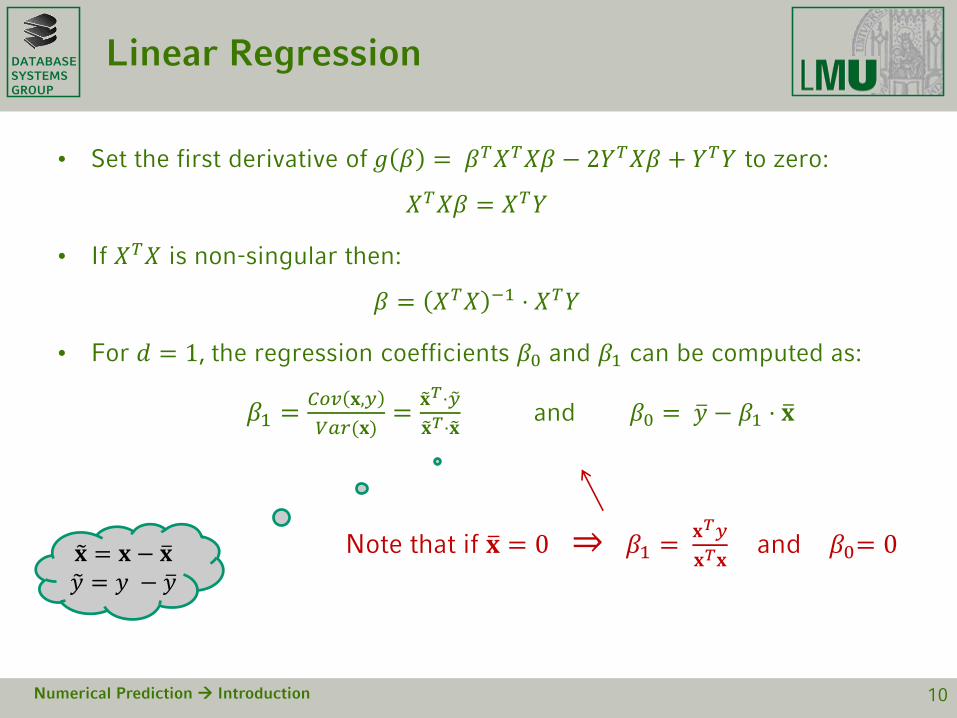
• Set the first derivative of 𝑔 𝛽 = 𝛽𝑇𝑋𝑇𝑋𝛽 − 2𝑌𝑇𝑋𝛽 + 𝑌𝑇𝑌 to zero:
𝑋𝑇𝑋𝛽 = 𝑋𝑇𝑌
• If 𝑋𝑇𝑋 is non-singular then:
𝛽 = 𝑋𝑇𝑋 −1 ⋅ 𝑋𝑇𝑌
• For 𝑑 = 1, the regression coefficients 𝛽0 and 𝛽1 can be computed as:
𝛽1 =𝐶𝑜𝑣 𝐱,𝑦
𝑉𝑎𝑟(𝐱)=
𝐱𝑇⋅ 𝑦
𝐱𝑇⋅𝐱and 𝛽0 = ത𝑦 − 𝛽1 ⋅ ത𝐱
Numerical Prediction Introduction 10
Note that if ത𝐱 = 0 ⇒ 𝛽1 =𝐱𝑇𝑦
𝐱𝑇𝐱and 𝛽0= 0𝐱 = 𝐱 − ത𝐱
𝑦 = 𝑦 − ത𝑦
DATABASESYSTEMSGROUP
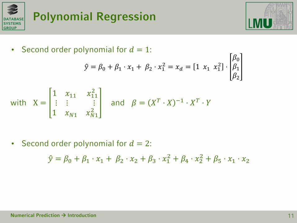
Polynomial Regression
• Second order polynomial for 𝑑 = 1:
with X =1 𝑥11 𝑥11
2
⋮ ⋮ ⋮1 𝑥𝑁1 𝑥𝑁1
2and 𝛽 = 𝑋𝑇 ⋅ 𝑋 −1 ⋅ 𝑋𝑇 ⋅ 𝑌
• Second order polynomial for 𝑑 = 2:
ො𝑦 = 𝛽0 + 𝛽1 ⋅ 𝑥1 + 𝛽2 ⋅ 𝑥2 + 𝛽3 ⋅ 𝑥12 + 𝛽4 ⋅ 𝑥2
2 + 𝛽5 ⋅ 𝑥1 ⋅ 𝑥2
Numerical Prediction Introduction 11
ො𝑦 = 𝛽0 + 𝛽1 ⋅ 𝑥1 + 𝛽2 ⋅ 𝑥12 = 𝑥𝑑 = 1 𝑥1 𝑥1
2 ⋅
𝛽0𝛽1𝛽2

DATABASESYSTEMSGROUP
Polynomial Regression
• The number of coefficients increases exponentially with 𝑘 and 𝑑
• Model building strategies: forward selection, backward elimination
• The order of the polynomial should be as low as possible, high order
polynomials tend to overfit the data
Numerical Prediction Introduction 12
Linear model Polynomial model 2𝑛𝑑 order Polynomial model 6𝑡ℎ order
0
0,5
1
1,5
2
2,5
3
3,5
4
4,5
0 2 4
0
0,5
1
1,5
2
2,5
3
3,5
4
4,5
0 2 4
0
1
2
3
4
5
0 2 4
DATABASESYSTEMSGROUP
Nonlinear Regression
• Different nonlinear functions can be approximated
• Transform the data to a linear domain
ො𝑦 = 𝜶 ⋅ 𝑒𝜸𝑥 ⇒ ln ො𝑦 = ln 𝛼 + 𝛾𝑥
⇒ ො𝑦′ = 𝛽0 + 𝛽𝑥
( for ො𝑦′ = ln ො𝑦 , 𝛽0 = ln 𝛼 , and 𝛽1 = 𝛾)
• The parameters 𝛽0 and 𝛽 are estimated with LS
• The parameters 𝜶 and 𝜸 are obtained, describing an exponential curve
which passes through the original observations
• Problem: LS determines normally distributed errors in the transformed
space ⇒ skewed error distribution in the original space
Numerical Prediction Introduction 13

DATABASESYSTEMSGROUP
Nonlinear Regression
• Different nonlinear functions can be approximated
• Outputs are estimated by a function with nonlinear parameters, e.g.,
exponential, trigonometric
• Example type of function:
ො𝑦 = 𝛽0 + 𝛽1𝑒𝛽2𝑥 + sin(𝛽3𝑥)
• Approach: the type of nonlinear function is chosen and the
corresponding parameters are computed
• No closed form solution exists ⇒ numerical approximations:
– Gauss Newton, Gradient descent, Levenberg-Marquardt
Numerical Prediction Introduction 14

DATABASESYSTEMSGROUP
Linear and Nonlinear Regression
• Problems:
– Linear regression – most of the real world data has a
nonlinear behavior
– Polynomial regression – limited, cannot describe
arbitrary nonlinear behavior
– General nonlinear regression – the type of nonlinear
function must be specified in advance
Numerical Prediction Introduction 15

DATABASESYSTEMSGROUP
Piecewise Linear Regression
• Piecewise linear functions:
𝑓 𝐱 = ቐ𝛽00 + 𝛽01 ⋅ 𝑥1 + …+ 𝛽0𝑑 ⋅ 𝑥𝑑 , 𝐱 ∈ ℘1
⋮𝛽𝑘0 + 𝛽𝑘1 ⋅ 𝑥1 + …+ 𝛽𝑘𝑑 ⋅ 𝑥𝑑 , 𝐱 ∈ ℘𝑘
• Simple approach
• Able to describe arbitrary functions
• The accuracy is increasing with an increasing number of
partitions/linear models
• The compactness & interpretability is increasing with a decreasing
number of partitions/ linear models
• Challenge: find an appropriate partitioning in the input space (number
and shapes)
Numerical Prediction Introduction 16
℘1 , … , ℘𝑘
are partitions in the input
space

DATABASESYSTEMSGROUP
Goals
1. Introduction of different learning techniques for piecewise linear models
2. Discussion of the bias-variance problem, regression and ensemble techniques
Classification Introduction 17
Training set Piecewise linear model with
regression trees
Continuous piecewise linear model with HH-
models
DATABASESYSTEMSGROUP
Chapter 7: Numerical Prediction
1) Introduction
– Numerical Prediction problem, linear and nonlinear
regression, evaluation measures
2) Piecewise Linear Numerical Prediction Models
– Regression Trees, axis parallel splits, oblique splits
– Hinging Hyperplane Models
3) Bias-Variance Problem
– Regularization , Ensemble methods
Numerical Prediction 18
DATABASESYSTEMSGROUP
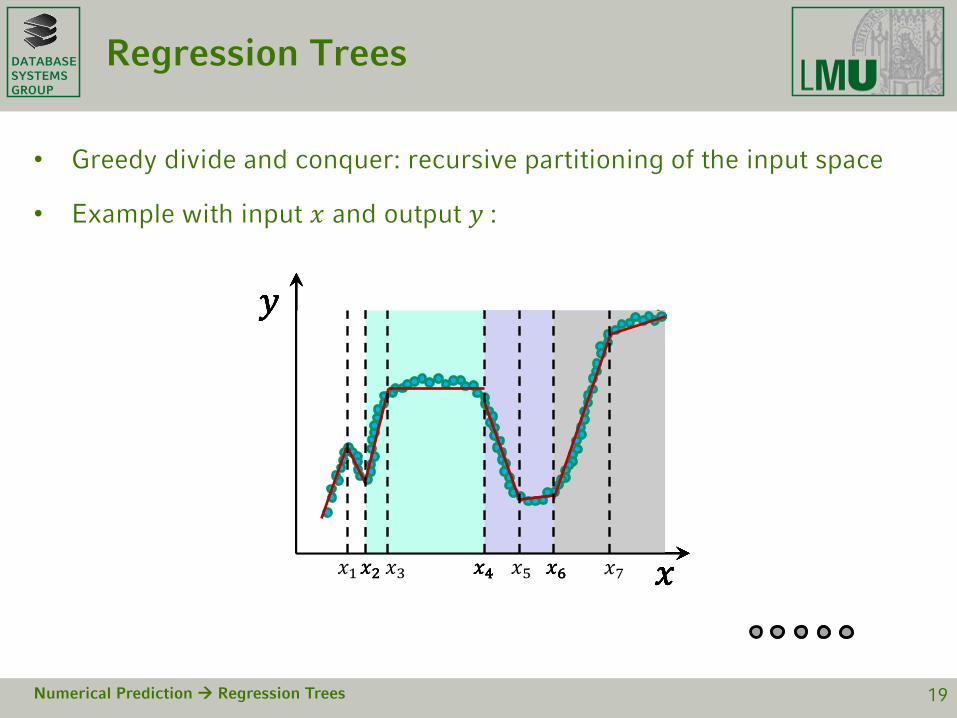
Regression Trees
• Greedy divide and conquer: recursive partitioning of the input space
• Example with input 𝑥 and output 𝑦 :
Numerical Prediction Regression Trees 19
𝑥
𝑦
𝑥
𝑦
𝑥4 𝑥
𝑦
𝑥
𝑦
𝑥
𝑦
𝑥2 𝑥4 𝑥6 𝑥
𝑦
𝑥2 𝑥4 𝑥6 𝑥
𝑦
𝑥1𝑥2 𝑥3 𝑥4 𝑥5 𝑥7𝑥6

DATABASESYSTEMSGROUP
Regression Trees
• Example:
Numerical Prediction Regression Trees 20
𝑥4
𝑥2
𝑥1 𝑥3
𝑥 < 𝑥2
𝑥 < 𝑥1
𝑥 ≥ 𝑥2
𝑥 < 𝑥3𝑥 ≥ 𝑥1 𝑥 ≥ 𝑥3
𝑥6
𝑥5 𝑥7
𝑥 < 𝑥6 𝑥 ≥ 𝑥6
𝑥 ≥ 𝑥7𝑥 < 𝑥7𝑥 < 𝑥5 𝑥 ≥ 𝑥5
DATABASESYSTEMSGROUP
Regression Trees
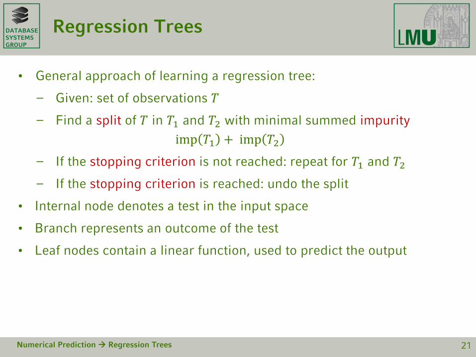
• General approach of learning a regression tree:
– Given: set of observations 𝑇
– Find a split of 𝑇 in 𝑇1 and 𝑇2 with minimal summed impurity
imp 𝑇1 + imp 𝑇2
– If the stopping criterion is not reached: repeat for 𝑇1 and 𝑇2
– If the stopping criterion is reached: undo the split
• Internal node denotes a test in the input space
• Branch represents an outcome of the test
• Leaf nodes contain a linear function, used to predict the output
Numerical Prediction Regression Trees 21
DATABASESYSTEMSGROUP
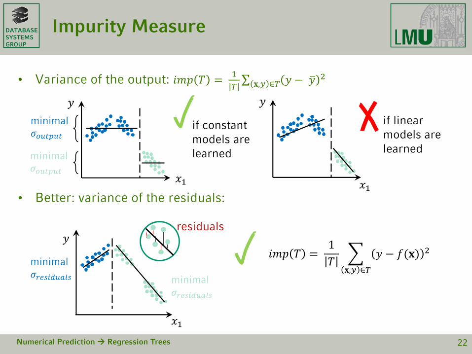
Impurity Measure
• Variance of the output: 𝑖𝑚𝑝 𝑇 =1
𝑇σ 𝐱,𝑦 ∈𝑇 𝑦 − ത𝑦 2
• Better: variance of the residuals:
Numerical Prediction Regression Trees 22
𝑥1
𝑦
𝑥1
𝑦
minimal 𝜎𝑜𝑢𝑡𝑝𝑢𝑡
𝑥1
𝑦
minimal 𝜎𝑟𝑒𝑠𝑖𝑑𝑢𝑎𝑙𝑠 minimal
𝜎𝑟𝑒𝑠𝑖𝑑𝑢𝑎𝑙𝑠
𝑖𝑚𝑝 𝑇 =1
𝑇
𝐱,𝑦 ∈𝑇
𝑦 − 𝑓(𝐱) 2
if constant models are learned
if linear models are learned
residuals
minimal 𝜎𝑜𝑢𝑡𝑝𝑢𝑡

DATABASESYSTEMSGROUP
Stopping Criterion: Impurity Ratio
• The recursive splitting is stopped if:
a) The sample size of a node is below a specified threshold
b) The split is not significant:
• If the relative impurity ratio induced by a split is higher than a
given threshold, then the split is not significant
• As the tree grows the resulting piecewise linear model gets more
accurate. 𝜏 increases, becoming higher than 𝜏0
• Choosing the parameter 𝜏0 ⇔ trading accuracy with overfitting
• stopping too soon ⇒ model is not accurate enough
• stopping too late ⇒ model overfits the observations
Numerical Prediction Regression Trees 23
𝜏 =𝑖𝑚𝑝 𝑇1 + 𝑖𝑚𝑝(𝑇2)
𝑖𝑚𝑝(𝑇)> 𝜏0

DATABASESYSTEMSGROUP
Split Strategy
• The split strategy determines how the training samples are partitioned,
whether the split is actually performed is decided by the stopping
criterion
• The most common splits are axis parallel:
– Split = a value in one input dimension
– Compute the impurity of all possible splits in all input dimensions and
choose at the end the split with the lowest impurity
– For each possible split compute the two corresponding models and their
impurity ⇒ expensive to compute
Numerical Prediction Regression Trees 24
𝑥1
𝑥2
4 axis parallel splits in the 2D input space, in
order to separate the red from the blue samples

DATABASESYSTEMSGROUP
Strategy for Oblique Splits
• More intuitive to use oblique splits
• An oblique split is a linear separator in the input space instead of a split
value in an input dimension
• The optimal split (with minimal impurity measure) cannot be efficiently
computed
• Heuristic approach required
Numerical Prediction Regression Trees 25
𝑥1
𝑥2
1 oblique split in the 2D input space, in order to separate the red from
the blue samples

DATABASESYSTEMSGROUP
Strategy for Oblique Splits
• Heuristic approach:
a) Compute a clustering in the full (input + output) space, such that the
samples are as well as possible described by linear equations
b) Project the clusters onto the input space
c) Use the clusters to train a linear classifier in the input space. Split =
separating hyperplane in input space
Numerical Prediction Regression Trees 26
𝑦
𝑥1
𝑥2
𝑦
𝑥1
𝑥2
𝑥1
𝑥2
a) b) & c)
DATABASESYSTEMSGROUP
Strategy for Oblique Splits
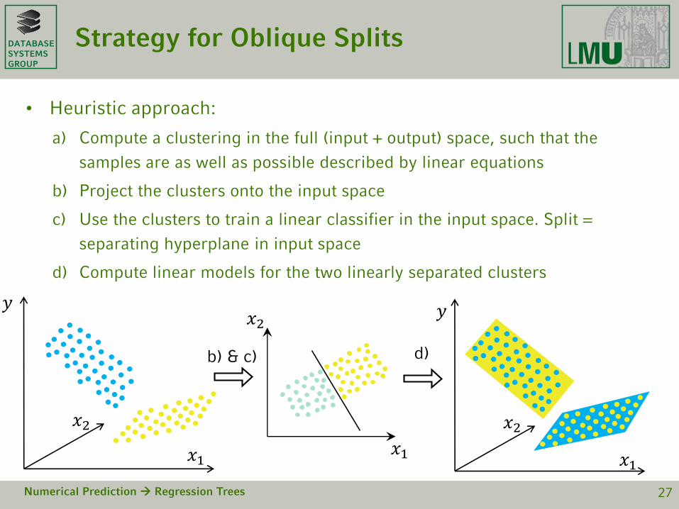
• Heuristic approach:
a) Compute a clustering in the full (input + output) space, such that the
samples are as well as possible described by linear equations
b) Project the clusters onto the input space
c) Use the clusters to train a linear classifier in the input space. Split =
separating hyperplane in input space
d) Compute linear models for the two linearly separated clusters
Numerical Prediction Regression Trees 27
𝑦
𝑥1
𝑥2
𝑥1
𝑥2
𝑥1
𝑥2
d)
𝑦
b) & c)

DATABASESYSTEMSGROUP
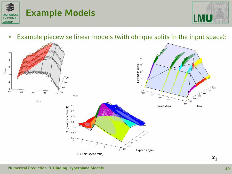
Example Models
• Example piecewise linear models (with oblique splits in the input space):
Numerical Prediction Regression Trees 28

DATABASESYSTEMSGROUP
Chapter 7: Numerical Prediction
1) Introduction
– Numerical Prediction problem, linear and nonlinear
regression, evaluation measures
2) Piecewise Linear Numerical Prediction Models
– Regression Trees, axis parallel splits, oblique splits
– Hinging Hyperplane Models
3) Bias-Variance Problem
– Regularization , Ensemble methods
Numerical Prediction 29
DATABASESYSTEMSGROUP
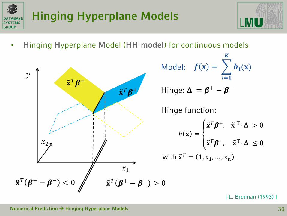
𝚫 = 𝜷+ − 𝜷−Hinge:
𝒇 𝐱 =
𝒊=𝟏
𝑲
𝒉𝒊(𝐱)Model:
Hinge function:
Hinging Hyperplane Models
• Hinging Hyperplane Model (HH-model) for continuous models
Numerical Prediction Hinging Hyperplane Models 30
ℎ 𝐱 = ൞𝐱𝑇𝜷+, 𝐱 𝐓⋅ 𝚫 > 0
𝐱𝑇𝜷−, 𝐱𝐓⋅ 𝚫 ≤ 0
with 𝐱𝑇 = 1, x1, … , x𝑛 .
𝐱𝑇𝜷−
𝐱𝑇𝜷+
𝐱𝑇 𝜷+ − 𝜷− < 0 𝐱𝑇 𝜷+ − 𝜷− > 0
𝑦
𝑥1
𝑥2
[ L. Breiman (1993) ]
DATABASESYSTEMSGROUP
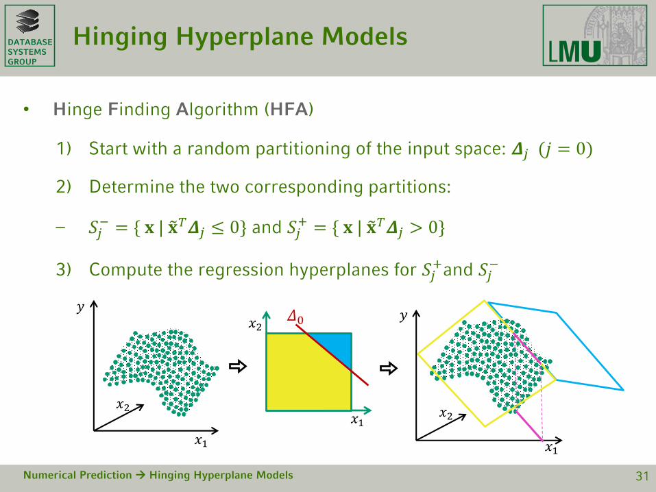
Hinging Hyperplane Models
• Hinge Finding Algorithm (HFA)
1) Start with a random partitioning of the input space: 𝜟𝑗 (𝑗 = 0)
2) Determine the two corresponding partitions:
– 𝑆𝑗− = { 𝐱 | 𝐱𝑇𝜟𝑗 ≤ 0} and 𝑆𝑗
+ = { 𝐱 | 𝐱𝑇𝜟𝑗 > 0}
3) Compute the regression hyperplanes for 𝑆𝑗+and 𝑆𝑗
−
Numerical Prediction Hinging Hyperplane Models 31
𝑥1
𝑥2
𝑦
𝑥1
𝑥2𝛥0
𝑥1
𝑥2
𝑦

DATABASESYSTEMSGROUP
Hinging Hyperplane Models
• Hinge Finding Algorithm (HFA)
3) Compute the regression hyperplanes for 𝑆𝑗+ and 𝑆𝑗
−
4) Compute the hinge 𝜟𝑗+1 from the regression coefficients 𝜷𝑗− and 𝜷𝑗
+
5) Determine the new partitions 𝑆𝑗+1+ and 𝑆𝑗+1
− determined by 𝜟𝑗+1
6) If 𝑆𝑗+1+ = 𝑆𝑗
+ or 𝑆𝑗+1+ = 𝑆𝑗
−, then stop, else return to step 3).
Numerical Prediction Hinging Hyperplane Models 32
𝑥1
𝑥2𝛥1
𝑥1
𝑥2
𝑦

DATABASESYSTEMSGROUP
Line Search for the Hinge Finding Algorithm
• The Hinge Finding Algorithm (HFA) might not converge – a hinge might
induce a partitioning outside the defined input space
• Line search: binary search to guarantee convergence (to a local
minimum)
• Instead of updating the hinge directly 𝜟𝑗 ⟶𝜟𝑗+1, first check the
accuracy improvement brought by 𝜟𝑗+1
• If 𝜟𝑗+1 does not improve the model impurity, then perform a binary
search after the linear combination of 𝜟𝑗 and 𝜟𝑗+1 yielding
the lowest impurity
𝜟′𝑗+1= 𝜟𝑖 + 𝜆 𝜟𝑗+1 − 𝜟𝑗 , 𝜆 ∈1
2,1
4,1
8,1
16
Numerical Prediction Hinging Hyperplane Models 33
𝑥1
𝑥2
𝛥𝑗
𝜟𝑗𝜟𝑗+1
DATABASESYSTEMSGROUP
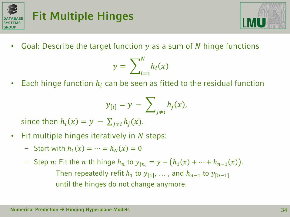
Fit Multiple Hinges
• Goal: Describe the target function 𝑦 as a sum of 𝑁 hinge functions
𝑦 = 𝑖=1
𝑁
ℎ𝑖 𝑥
• Each hinge function ℎ𝑖 can be seen as fitted to the residual function
𝑦 𝑖 = 𝑦 − 𝑗≠𝑖
ℎ𝑗 𝑥 ,
since then ℎ𝑖 𝑥 = 𝑦 − σ𝑗≠𝑖 ℎ𝑗(𝑥).
• Fit multiple hinges iteratively in 𝑁 steps:
– Start with ℎ1 𝑥 = ⋯ = ℎ𝑁 𝑥 = 0
– Step 𝑛: Fit the 𝑛-th hinge ℎ𝑛 to 𝑦 𝑛 = 𝑦 − ℎ1 𝑥 + ⋯+ ℎ𝑛−1 𝑥 .
Then repeatedly refit ℎ1 to 𝑦 1 , … , and ℎ𝑛−1 to 𝑦[𝑛−1]
until the hinges do not change anymore.
Numerical Prediction Hinging Hyperplane Models 34

DATABASESYSTEMSGROUP
Fit Multiple Hinges
• Example:
– Step 1: Fit the first hinge function ℎ1 to 𝑦 1 = 𝑦 − 0.
– Step 2: Compute the residual outputs
𝑦[2] = 𝑦 − ℎ1 𝑥 .
Fit the second hinge function ℎ2 to 𝑦[2].
Then refit the first hinge to 𝑦[1] = 𝑦 − ℎ2(𝑥).
– Step 3: Compute the residual outputs
𝑦[3] = 𝑦 − ℎ1 𝑥 − ℎ2 𝑥 .
Fit the third hinge function ℎ3 to 𝑦 3 .
Then repeatedly refit
ℎ1 to 𝑦[1] = 𝑦 − ℎ2 𝑥 − ℎ3 𝑥 and
ℎ2 on 𝑦[2] = 𝑦 − ℎ1 𝑥 − ℎ3 𝑥 .
until no more changes occur.
Numerical Prediction Hinging Hyperplane Models 35
DATABASESYSTEMSGROUP
Example Models
• Example piecewise linear models (with oblique splits in the input space):
Numerical Prediction Hinging Hyperplane Models 36
𝑥1
DATABASESYSTEMSGROUP
Chapter 7: Numerical Prediction
1) Introduction
– Numerical Prediction problem, linear and nonlinear
regression, evaluation measures
2) Piecewise Linear Numerical Prediction Models
– Regression Trees, axis parallel splits, oblique splits
– Hinging Hyperplane Models
3) Bias-Variance Problem
– Regularization , Ensemble methods
37
DATABASESYSTEMSGROUP
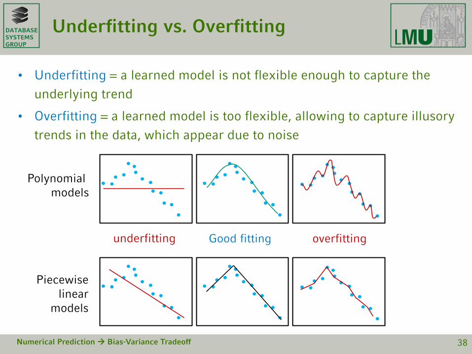
Underfitting vs. Overfitting
• Underfitting = a learned model is not flexible enough to capture the
underlying trend
• Overfitting = a learned model is too flexible, allowing to capture illusory
trends in the data, which appear due to noise
Numerical Prediction Bias-Variance Tradeoff 38
Polynomial models
Piecewise linear
models
underfitting Good fitting overfitting
DATABASESYSTEMSGROUP
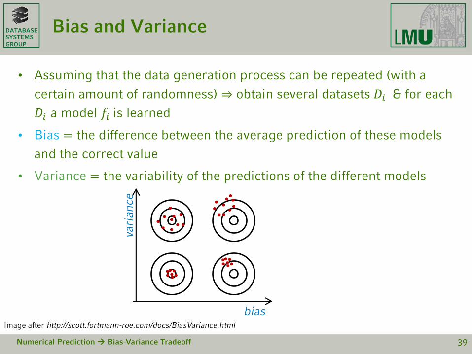
Bias and Variance
• Assuming that the data generation process can be repeated (with a
certain amount of randomness) ⇒ obtain several datasets 𝐷𝑖 & for each
𝐷𝑖 a model 𝑓𝑖 is learned
• Bias = the difference between the average prediction of these models
and the correct value
• Variance = the variability of the predictions of the different models
Numerical Prediction Bias-Variance Tradeoff 39
bias
vari
an
ce
Image after http://scott.fortmann-roe.com/docs/BiasVariance.html

DATABASESYSTEMSGROUP
Bias-Variance Tradeoff
• Underfitting = low variance, high bias (e.g. use mean output as estimator)
• High bias = a model does not approximate the underlying function well
• Overfitting = high variance, low bias
• When a model is too complex, small changes in the data cause the predicted
value to change a lot ⇒ high variance
• Search for the best tradeoff between bias and variance
• Regression: control the bias-variance tradeoff by means of the polynomial
order/number of coefficients
• Regression trees: control the bias-variance tradeoff by means of the tree
size/number of submodels
Numerical Prediction Bias-Variance Tradeoff 40

DATABASESYSTEMSGROUP
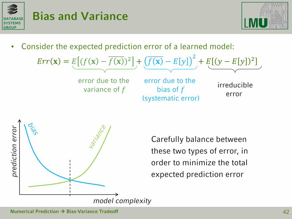
Bias and Variance
• Consider the expected prediction error of a learned model:
𝐸𝑟𝑟(𝐱) = 𝐸 𝑓 𝐱 − 𝑦 2
𝐸𝑟𝑟(𝐱) = 𝐸 𝑓 𝐱 2 − 2𝑓 𝐱 𝑦 + 𝑦2
𝐸𝑟𝑟 𝐱 = 𝐸 𝑓 𝐱 2 − 2𝐸 𝑓 𝐱 𝐸 𝑦 + 𝐸 𝑦2
𝐸𝑟𝑟 𝐱 = 𝐸 (𝑓 𝐱 − 𝑓 𝐱 )2 + 𝑓 𝐱 2 − 2𝑓 𝐱 𝐸 𝑦 + 𝐸 𝑦 − 𝐸 𝑦 2 + 𝐸 𝑦 2
𝐸𝑟𝑟 𝐱 = 𝐸 (𝑓 𝐱 − 𝑓 𝐱 )2 + 𝑓 𝐱 − 𝐸 𝑦2+ 𝐸 𝑦 − 𝐸 𝑦 2
Numerical Prediction Bias-Variance Tradeoff 41
(⋆): 𝐸 𝑧2 = 𝐸 (𝑧 − 𝐸[𝑧])2 + 𝐸[𝑧]2
error due to the variance of 𝑓
error due to the bias of 𝑓
(systematic error)
irreducibleerror
(⋆)
DATABASESYSTEMSGROUP
Bias and Variance
• Consider the expected prediction error of a learned model:
𝐸𝑟𝑟 𝐱 = 𝐸 (𝑓 𝐱 − 𝑓 𝐱 )2 + 𝑓 𝐱 − 𝐸 𝑦2+ 𝐸 𝑦 − 𝐸 𝑦 2
Numerical Prediction Bias-Variance Tradeoff 42
error due to the variance of 𝑓
error due to the bias of 𝑓
(systematic error)
Carefully balance between
these two types of error, in
order to minimize the total
expected prediction error
model complexity
pre
dic
tion
err
or
irreducibleerror
DATABASESYSTEMSGROUP
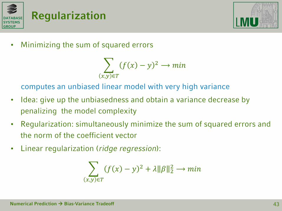
Regularization
• Minimizing the sum of squared errors
𝑥,𝑦 ∈𝑇
𝑓 𝑥 − 𝑦 2 ⟶𝑚𝑖𝑛
computes an unbiased linear model with very high variance
• Idea: give up the unbiasedness and obtain a variance decrease by
penalizing the model complexity
• Regularization: simultaneously minimize the sum of squared errors and
the norm of the coefficient vector
• Linear regularization (ridge regression):
𝑥,𝑦 ∈𝑇
𝑓 𝑥 − 𝑦 2 + 𝜆 𝛽 22 ⟶𝑚𝑖𝑛
Numerical Prediction Bias-Variance Tradeoff 43

DATABASESYSTEMSGROUP
Regularization
• Lasso regularization:
argmin𝛽
𝑥,𝑦 ∈𝑇
𝑓 𝑥 − 𝑦 2, 𝑠. 𝑡. 𝛽 1 ≤ 𝑠
– solvable with a quadratic programming algorithm
– With an increasing penalty more and more coefficients
are shrunk towards zero, generating more sparse models
• Linear regularization (ridge regression):
argmin𝛽
𝑥,𝑦 ∈𝑇
𝑓 𝑥 − 𝑦 2, 𝑠. 𝑡. 𝛽 22 ≤ 𝑠
– solvable similar to SSE: 𝛽 = 𝑋𝑇𝑋 + 𝜆𝐼 −1 ⋅ 𝑋𝑇𝑌
– Reduces all coefficients simultaneously
Numerical Prediction Bias-Variance Tradeoff 44
𝛽1
𝛽2
𝛽1
𝛽2constraint region
unregularizederror function
DATABASESYSTEMSGROUP
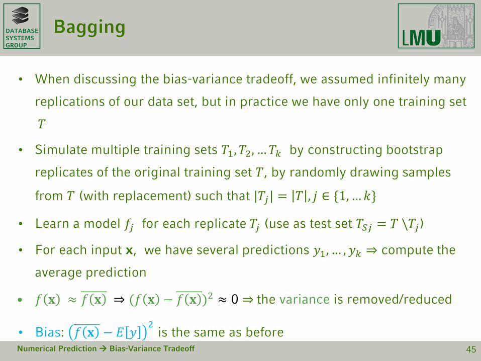
Bagging
• When discussing the bias-variance tradeoff, we assumed infinitely many
replications of our data set, but in practice we have only one training set
𝑇
• Simulate multiple training sets 𝑇1, 𝑇2, … 𝑇𝑘 by constructing bootstrap
replicates of the original training set 𝑇, by randomly drawing samples
from 𝑇 (with replacement) such that |𝑇𝑗| = 𝑇 , 𝑗 ∈ {1, …𝑘}
• Learn a model 𝑓𝑗 for each replicate 𝑇𝑗 (use as test set 𝑇𝑆𝑗 = 𝑇 \𝑇𝑗)
• For each input x, we have several predictions 𝑦1, … , 𝑦𝑘 ⇒ compute the
average prediction
• 𝑓 𝐱 ≈ 𝑓 𝐱 ⇒ (𝑓 𝐱 − 𝑓 𝐱 )2 ≈ 0 ⇒ the variance is removed/reduced
• Bias: 𝑓 𝐱 − 𝐸 𝑦2
is the same as beforeNumerical Prediction Bias-Variance Tradeoff 45

DATABASESYSTEMSGROUP
Ensemble Methods
• Bagging:
– use it for models with a low bias
– If the bias is low, bagging reduces the variance, while bias remains
the same
– use it for complex models, which tend to overfit the training data
– in practice it might happen that the bagging approach slightly
increases the bias
• Boosting:
– Can be adapted for regression models
– Reduces the bias in the first iterations
– Reduces the variance in later iterations
Numerical Prediction Bias-Variance Tradeoff 46