Embed Size (px)
Citation preview
Objectives
© E
MP
IPE
20
09/U
SE
D U
ND
ER
LIC
EN
SE
FR
OM
SH
UT
TE
RS
TO
CK
.CO
M
263
Standard Costing and Variance Analysis
After completing this chapter, you should be able to answer the following questions:
LO.1 How are material, labor, and overhead standards set?LO.2 How are material, labor, and overhead variances calculated and recorded?LO.3 Why are standard cost systems used?LO.4 How have the setting and use of standards changed over time?LO.5 How does the use of a single conversion element (rather than the
traditional labor and overhead elements) aff ect standard costing?LO.6 (Appendix) How are variances aff ected by multiple material and labor
categories?
7

264 Chapter 7 Standard Costing and Variance Analysis
LO.1 How are material, labor, and overhead standards set?
IntroductionAs discussed in Chapter 5, a standard is a performance benchmark. Organizations develop and use standards for almost all tasks. For example, businesses set standards for employee sales expenses, hotels set standards for performing housekeeping tasks and delivering room service, and casinos set standards for revenue to be generated per square foot of playing space. McDonald’s standards state that 1 pound of beef will provide 10 hamburger patties, a bun will be toasted for 17 seconds, and one packet of sanitizer will be used for every 2.5 gallons of water when cleaning the shake machine.1
Because of the variety of organizational activities and information objectives, no single standard costing system is appropriate for all situations. Some systems use standards for costs but not for quantities; other systems (especially those in service businesses) use stan-dards for labor but not material. Accountants help explain the fi nancial consequences of exceeding or failing to achieve target performance levels. Without a predetermined measure, managers have no way of knowing what performance level is expected. And, without comparing the actual result to the predetermined measure, managers have no way of knowing whether the company met expectations or of exercising control.
Th is chapter discusses a traditional standard cost system that provides price and quantity standards for each cost component: direct material, direct labor, and manufacturing overhead. Th e chapter discusses how standards are developed, how variances from standards are calcu-lated, and what information can be gained from variance analysis. Journal entries used in a standard cost system are shown. Th e chapter appendix covers mix and yield variances that can arise from using multiple types of materials or groups of labor.
Development of a Standard Cost SystemAlthough manufacturing companies originally initiated the use of standard cost systems, ser-vice and not-for-profi t organizations also use standards. A standard cost system tracks both standard and actual costs in the accounting records. Th is dual recording provides an essen-tial element of cost control: having norms against which actual operations can be compared. Standard cost systems use standards, which specify the expected costs and quantities needed to manufacture a single unit of product or perform a single service. Developing a standard cost involves judgment and practicality in identifying the material and labor types, quantities, and prices as well as understanding the types of organizational overhead and how they behave.
A primary objective in manufacturing a product is to minimize unit cost while achieving certain quality specifi cations. Almost all products can be manufactured from a variety of alternative inputs that would generate similar output and output quality. Th e input choices that are made aff ect the standards that are set.
Some possible input resource combinations are not necessarily practical or effi cient. For instance, a labor team might consist only of craftspersons or skilled workers, but such a team might not be cost benefi cial if the wage rates of skilled and unskilled workers diff er signifi cantly. Also, providing high-technology equipment to unskilled labor is possible, but doing so would not be an effi cient use of resources.
After the desired output quality and the input resources needed to achieve that quality at a reasonable cost have been determined, price and quantity standards can be developed. Experts from cost accounting, industrial engineering, human resources, data processing, purchasing, and management contribute information and expertise toward developing standards. Inclusion of the various groups helps to ensure credibility of the standards and to motivate people to achieve the standards. Th e discussion of the standard-setting process begins with material.
1 Daniel Kruger, “You Want Data with That?” Forbes (March 29, 2004), pp. 58–59.

Chapter 7 Standard Costing and Variance Analysis 265
Material Standards
Th e fi rst step in developing material standards is to identify and list the specifi c direct material(s) needed to manufacture the product. Th is list is generally available on product specifi cation documents prior to initial production. Without such documentation, material specifi cations can be determined by observing the production area, questioning production personnel, inspecting material requisitions, and reviewing the product-related cost accounts. Four things must be known about material inputs:
type of material needed,•
quality (grade) of material needed,•
quantity of material needed, and•
price per unit of material (must be based on level of quality specifi ed).•
For example, the direct material used in producing a baseball glove is cured and tanned leather; indirect materials include nylon thread and small plastic reinforcements at the base of the thumb and small fi nger. Because only about 30 percent of a cowhide can actually be used to make baseball gloves, each cowhide provides enough leather for only three or four gloves—but actual output depends on the glove size being produced (from gloves worn to play T-ball to those worn in the major leagues). Buff alo hide, kangaroo hide, pigskin, and man-made materi-als may be substituted for cowhide, but choice of material will aff ect the cost of the material.2
In making quality decisions, managers should remember that as the material grade rises, so generally does price; decisions about material inputs usually seek to balance the relationships of price, quality, and projected selling prices with company objectives. Th e resulting trade-off s aff ect material mix, material yield, fi nished product quality and quan-tity, overall product cost, and product salability. Th us, quantity and cost estimates become direct functions of quality decisions. Tanning is important in the manufacturing process of baseball gloves because that process is what provides the gloves with their fl exibility and durability; if hides are not properly tanned, the gloves quickly crack and fl ake. Only after the quality level is selected for each component can estimates be made for the physical quantity of weight, size, volume, or other input measure(s). Th ese estimates are based on the results of engineering tests, opinions of managers and workers using the material, past material requisitions, and review of the cost accounts.
Unlike baseball gloves, most products require multiple direct material inputs. Th e speci-fi cations for materials, including quality and quantity, are compiled on a product’s bill of materials. Exhibit 7–1 (p. 266) shows the bill of materials for one type of mountain bike manufactured by Sanjay Corporation. Even companies without formal standard cost sys-tems develop bills of materials for products as guides for production activity.
When converting quantities from the bill of materials into costs, companies often make allowances for normal waste of components.3 After standard quantities have been developed, component prices must be determined. Purchasing agents may be able to exercise substantial infl uence on input prices in the following ways:
understanding the quantity and timing of company purchasing;•
knowing what alternative suppliers are available;•
recognizing the economic climate under which purchases are being made;•
performing “due diligence” as to the input costs incurred and profi t margins desired by • suppliers; and
when appropriate, seeking single source suppliers or partnership alliances with suppliers.•
Rather than considering only the direct purchase price of an input, purchasing agents now try to estimate and minimize the total cost of ownership (TCO), which includes price,
2 http://www.madehow.com/Volume-1/Baseball-Glove.html.3 Although such allowances are often made, providing for them does not result in the most effective use of a standard cost system. Problems arising from including such allowances are discussed later in this chapter.

266 Chapter 7 Standard Costing and Variance Analysis
freight/duty/tax charges, payment and discount terms, inventory storage costs, scrap rates, rebates or special incentives, warranties, and disposal costs. Incorporating such information into price standards should make it easier for the purchasing agent to later determine the causes of any signifi cant diff erences between actual and standard prices.
When all quantity and price information is available, component quantities are multi-plied by unit prices to obtain each component’s total cost. (Remember that cost equals price times quantity.) Th ese totals are summed to determine the total standard material cost of one unit of product.
Labor Standards
Developing labor standards requires the same basic procedures as those used for mate-rial. Each production operation performed by workers (such as bending, reaching, lifting, moving material, and packing) or by machinery (such as drilling, cooking, and assembling) should be identifi ed. In specifying operations and movements, activities such as cleanup, setup, and rework are considered. All unnecessary movements of workers and material should be disregarded when time standards are set.
To develop eff ective standards, a company obtains quantitative information for each pro-duction operation. Such information can be gathered from industrial engineering methods, in-house time-and-motion studies, or historical data. Methods-time measurement (MTM) is an industrial engineering process that analyzes work tasks to determine the time a trained worker requires to perform a given operation at a rate that can be sustained for an 8-hour workday. In-house studies may result in employees engaging in “slowdown” tactics when they are being monitored. Such tactics result in a longer time being established as the standard,
Product Name: Mountain Bike (unassembled)Product # 15Date Established: January 10, 2010
COMPONENT ID# QUANTITY REQUIRED DESCRIPTION COMMENTS
WF-05 1 Front wheel, Stumpjumper tire & tube
WR-05 1 Rear wheel, Stumpjumper tire & tube
B-05 2 Front & rear Includes brakes derailleur, levers, and calipers HB-05 1 Handlebar and Stainless steel stem
B-21 16 2.5" x 5/16" bolts Includes nuts and flat washers
S-18 12 3" clamps Stainless steel
SPS-05 1 Seat post and Nylon and black seat
P-05 2 Pedals Black rubber
F-05 1 Frame Fiberglass
Exhibit 7–1 Sanjay Corporation’s Bill of Materials
Chapter 7 Standard Costing and Variance Analysis 267
which makes employees appear more effi cient when actual results are measured. Slowdowns may also occur because employees, knowing they are being observed, want to make certain that they are performing the task correctly. Rather than monitoring task performance, the average time needed to manufacture a product during the prior year can be calculated from employee time sheets and used to set a current time standard. A problem with this method is that histori-cal data can include ineffi ciencies. To compensate for biases in internal estimates, management and supervisory personnel normally adjust standards for slowdowns or past ineffi ciencies by making subjective adjustments to any internal information gathered.
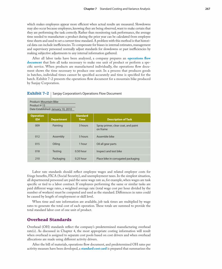
After all labor tasks have been analyzed, a company prepares an operations fl ow document that lists all tasks necessary to make one unit of product or perform a spe-cifi c service. When products are manufactured individually, the operations fl ow docu-ment shows the time necessary to produce one unit. In a process that produces goods in batches, individual times cannot be specifi ed accurately and time is specifi ed for the batch. Exhibit 7–2 presents the operations fl ow document for a mountain bike produced by Sanjay Corporation.
Product: Mountain BikeProduct # 15Date Established: January 10, 2010
Operation ID# Department Description of Task
009
012
015
018
210
Painting
Assembly
Oiling
Testing
Packaging
3 hours
5 hours
1 hour
0.50 hour
0.25 hour
Spray primer, clear coat, and paint on frame
Assemble bike
Oil all gear parts
Inspect and test bike
Place bike in corrugated packaging
StandardTime
Exhibit 7–2 Sanjay Corporation’s Operations Flow Document
Labor rate standards should refl ect employee wages and related employer costs for fringe benefi ts, FICA (Social Security), and unemployment taxes. In the simplest situation, all departmental personnel are paid the same wage rate as, for example, when wages are task specifi c or tied to a labor contract. If employees performing the same or similar tasks are paid diff erent wage rates, a weighted average rate (total wage cost per hour divided by the number of workers) must be computed and used as the standard. Diff erences in rates could be caused by length of employment or skill level.
When time and rate information are available, job task times are multiplied by wage rates to generate the total cost of each operation. Th ese totals are summed to provide the total standard labor cost of one unit of product.
Overhead Standards
Overhead (OH) standards refl ect the company’s predetermined manufacturing overhead rate(s). As discussed in Chapter 4, the most appropriate costing information will result when overhead is assigned to separate cost pools based on cost drivers and when overhead allocations are made using diff erent activity drivers.
After the bill of materials, operations fl ow document, and predetermined OH rates per activity measure have been developed, a standard cost card is prepared that summarizes the

268 Chapter 7 Standard Costing and Variance Analysis
standard quantities and costs needed to produce a unit. Th e standard cost card for Sanjay Corporation’s mountain bike is shown in Exhibit 7–3. For simplicity, it is assumed that Sanjay Corporation uses only two predetermined overhead rates: one for variable manufac-turing costs and one for fi xed manufacturing costs.
Product: Mountain BikeProduct # 15Date Established: January 10, 2010
Component ID# Quantity Required Unit Cost
DIRECT MATERIAL
ID#TotalHrs Painting Assembling
TotalCost
WageRate/Hr
009 $12 3.00 $36 $ 36
012 15 5.00 $75 75
015 8 1.00 $8 8
Testing 20 0.50 $10 10
Packaging 8 0.25 $2 2
Totals 9.75 $36 $75 $8 $10 $2 $131
$136.5097.50
$234.00
Total Cost
Oiling Testing Packaging
DIRECT LABOR
WF-05 1 $ 20.00 $ 20
WR-05 1 25.00 25
B-05 2 20.00 40
HB-05 1 23.00 23
B-21 16 0.75 12
S-18 12 1.25 15
SPS-05 1 17.00 17
P-05 2 14.00 28
F-05 1 200.00 200
Total cost $380
Expected capacity for 2010: 5,000 bikes
Expected capacity in DLHs for 2010 = 5,000 bikes × 9.75 = 48.75 DLHs
MANUFACTURING OVERHEAD
Variable overhead ($682,500 + 48.70 = $14 × 9.75 DLH per bike)
Fixed overhead ($587,500 + 48,750 = 510 per DLH; $10 × 9.75 DLH per bike)
Total overhead
Exhibit 7–3 Sanjay Corporation’s Standard Cost Card for a Mountain Bike
Although both actual and standard costs are recorded in a standard cost system, only standard costs are shown in the Raw (Direct) Material, Work in Process, and Finished Goods Inventory accounts. Th e standard cost of each cost element (direct material, direct labor, vari-able overhead, and fi xed overhead) is said to be “applied” or “allocated” to the goods produced. Th is terminology is the same as that used when overhead is assigned to inventory based on a predetermined rate. A variance is any diff erence between an actual cost and a standard cost.

Chapter 7 Standard Costing and Variance Analysis 269
LO.2 How are material, labor, and overhead variances calculated and recorded?
General Variance Analysis ModelA total variance is the diff erence between the total actual cost for the production inputs and the total standard cost applied to the production output. Th is variance can be dia-grammed as follows:
Actual Cost of Actual Input
Standard Cost of Actual Output
Total Variance
Total variances do not provide useful information for determining why standard and actual costs diff ered. For instance, the preceding variance computation does not indicate whether the variance was caused by price factors, quantity factors, or both. To provide additional information, total variances are subdivided into price and usage components. Th e total vari-ance diagram can be expanded to provide the following general model indicating the two subvariances:
Th e price component indicates the diff erence between what was actually paid for inputs and the amount expected to be paid for inputs. Th e price (or rate) variance is calculated as the diff erence between the actual price (AP) and the standard price (SP) per unit of input multiplied by the actual input quantity (AQ):
Price (or Rate) Variance � (AP � SP)(AQ)
Th e diagram of the general model moves from actual cost of actual input quantity in the left column to standard cost of actual output in the right column. Th e change from input to output refl ects the fact that the actual ratio of inputs to outputs will not necessarily equal the standard ratio of inputs to outputs. Th e model’s middle column refl ects actual quantity and standard price.
Th e usage component of the total variance shows the effi ciency of results or the rela-tionship of input to output. Th e model’s far right column shows total standard cost, which refl ects a measure of output known as the standard quantity. Th is quantity translates actual production output into the standard input quantity: the quantity that should have been used to achieve that output. Th e monetary amount shown in the right-hand column of the general variance analysis model is computed as the standard quantity multiplied by the standard input price. Th is computation provides a monetary measure that can be recorded in the accounting records. Th e quantity/effi ciency variance is calculated as the diff erence between the AQ and standard quantity of input allowed (SQ) multiplied by the standard price per unit of input:
Quantity (or Efficiency) Variance � (AQ � SQ)(SP)
If the actual price or quantity amounts are higher than the standard price or quantity amounts, the variance is unfavorable (U); if the actual amounts are lower than the standard amounts, the variance is favorable (F). An unfavorable variance has a negative eff ect on income, and a favorable variance has a positive eff ect on income.
Actual Cost of Actual Quantity
of Inputs
Standard Cost of Actual Quantity
of Inputs
Standard Cost of Standard Quantity of Inputs Allowed
Price Component
Price/Rate Variance
Usage Component
Quantity/Effi ciency Variance
Total Variance
270 Chapter 7 Standard Costing and Variance Analysis
Actual to Standard Relationship Variance Effect on Income
Actual Price � Standard Price Unfavorable Negative
Actual Price � Standard Price Favorable Positive
Actual Quantity � Standard Quantity Unfavorable Negative
Actual Quantity � Standard Quantity Favorable Positive
It is important to note, however, that unfavorable is not necessarily equated with bad nor is favorable equated with good. Determination of “bad” or “good” must be made after identifying the cause of the variance and the implications of that variance for other cost elements.
Th e following sections illustrate variance computations for each cost element.
Material and Labor Variance ComputationsDuring January 2010, Sanjay Corporation produced 400 mountain bikes (the actual quan-tity made by Sanjay Corporation in January 2010). Th e top half of Exhibit 7–4 shows the standard quantities and costs for that production, while the bottom half of the exhibit shows actual quantities and costs. Th is information is used to compute the January 2010 variances.
Material Variances
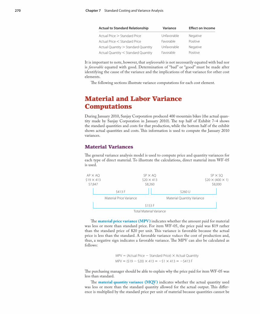
Th e general variance analysis model is used to compute price and quantity variances for each type of direct material. To illustrate the calculations, direct material item WF-05 is used.
Th e material price variance (MPV) indicates whether the amount paid for material was less or more than standard price. For item WF-05, the price paid was $19 rather than the standard price of $20 per unit. Th is variance is favorable because the actual price is less than the standard. A favorable variance reduces the cost of production and, thus, a negative sign indicates a favorable variance. Th e MPV can also be calculated as follows:
MPV � (Actual Price � Standard Price) � Actual Quantity
MPV � ($19 � $20) � 413 � �$1 � 413 � �$413 F
Th e purchasing manager should be able to explain why the price paid for item WF-05 was less than standard.
Th e material quantity variance (MQV) indicates whether the actual quantity used was less or more than the standard quantity allowed for the actual output. Th is diff er-ence is multiplied by the standard price per unit of material because quantities cannot be
AP � AQ$19 � 413
$7,847
SP � AQ$20 � 413
$8,260
SP � SQ$20 � (400 � 1)
$8,000
$413 F $260 U
Material Price Variance Material Quantity Variance
$153 F
Total Material Variance

Chapter 7 Standard Costing and Variance Analysis 271
Exhibit 7–4 Standard and Actual Cost Data for Sanjay Corporation’s January 2010 Production of 400 Mountain Bikes
STANDARD COST FOR 400 MOUNTAIN BIKES
Direct Material Component ID# Quantity Unit Cost Total CostWF-05 400 $ 20.00 $ 8,000WR-05 400 25.00 10,000B-05 800 20.00 16,000HB-05 400 23.00 9,200B-21 6,400 0.75 4,800S-18 4,800 1.25 6,000SPS-05 400 17.00 6,800P-05 800 14.00 11,200F-05 400 200.00 80,000 Total standard direct material cost $152,000
Direct LaborDepartment Total Hours Rate Total CostPainting 1,200 $12.00 $14,400Assembling 2,000 15.00 30,000Oiling 400 8.00 3,200Testing 200 20.00 4,000Packaging 100 8.00 800 Total standard direct labor hours and cost 3,900 $52,400
Variable overhead (9.75 DLM per bike � $14 per DLH � $136.50 per bike � 400 bikes) $54,600Fixed overhead ($9.750 per bike � 400 bikes) 39,000 Total standard overhead cost $93,600
ACTUAL JANUARY COST FOR 400 MOUNTAIN BIKES
Direct MaterialComponent ID# Quantity Unit Cost Total CostWF-05 413 $ 19.00 $ 7,847WR-05 400 24.00 9,600B-05 810 20.00 16,200HB-05 400 24.00 9,600B-21 6,700 0.74 4,958S-18 4,850 1.20 5,820SPS-05 400 18.00 7,200P-05 800 15.00 12,000F-05 400 197.00 78,800 Total actual direct material cost $152,025
Direct LaborDepartment Total Hours Rate Total Cost
Painting 1,100 $12.00 $13,200Assembling 1,900 16.00 30,400Oiling 390 7.90 3,081Testing 200 19.50 3,900Packaging 90 8.00 720 Total actual direct labor hours and cost 3,680 $51,301
Variable overhead $50,784Fixed overhead 38,500 Total actual overhead cost $89,284
272 Chapter 7 Standard Costing and Variance Analysis
entered into the accounting records. Production used 13 more units of WF-05 than the standard allowed, resulting in a $260 unfavorable material quantity variance. Th e MQV can be calculated as follows:
MQV � Standard Price � (Actual Quantity � Standard Quantity)
MQV � $20 � (413 � 400) � $20 � 13 � $260 U
Th e production manager should be able to explain why the additional WF-05 components were used in January.
Th e total material variance (TMV) is the summation of the individual variances or can also be calculated by subtracting the total standard cost for component WF-05 from the total actual cost of WF-05:
TMV � MPV � MQV � �$413 � $260 � �$153 (or $153 F)
or
TMV � Total actual cost � Total standard cost � $7,847 � $8,000 � �$153 (or $153 F)
Price and quantity variance computations must be made for each direct material component and these component variances are summed to obtain the total price and quantity variances. Such a summation, however, does not provide useful information for cost control.
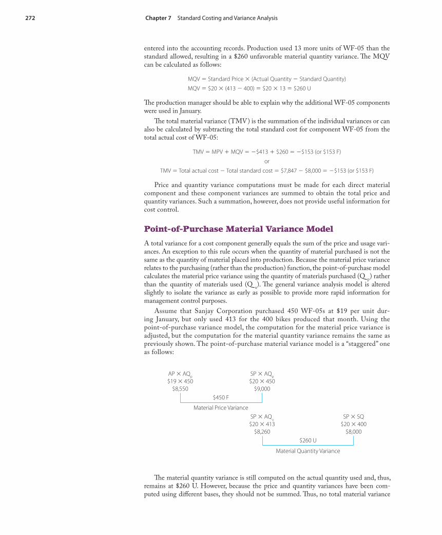
Point-of-Purchase Material Variance Model
A total variance for a cost component generally equals the sum of the price and usage vari-ances. An exception to this rule occurs when the quantity of material purchased is not the same as the quantity of material placed into production. Because the material price variance relates to the purchasing (rather than the production) function, the point-of-purchase model calculates the material price variance using the quantity of materials purchased (Q
p) rather
than the quantity of materials used (Qu). Th e general variance analysis model is altered
slightly to isolate the variance as early as possible to provide more rapid information for management control purposes.
Assume that Sanjay Corporation purchased 450 WF-05s at $19 per unit dur-ing January, but only used 413 for the 400 bikes produced that month. Using the point-of-purchase variance model, the computation for the material price variance is adjusted, but the computation for the material quantity variance remains the same as previously shown. The point-of-purchase material variance model is a “staggered” one as follows:
AP � AQp
$19 � 450$8,550
SP � AQp
$20 � 450$9,000
$450 F
Material Price VarianceSP � AQu
$20 � 413$8,260
SP � SQ$20 � 400
$8,000$260 U
Material Quantity Variance
Th e material quantity variance is still computed on the actual quantity used and, thus, remains at $260 U. However, because the price and quantity variances have been com-puted using diff erent bases, they should not be summed. Th us, no total material variance
Chapter 7 Standard Costing and Variance Analysis 273
can be meaningfully determined when the quantity of material purchased diff ers from the quantity of material used.
Labor Variances
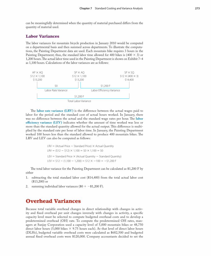
Th e labor variances for mountain bicycle production in January 2010 would be computed on a departmental basis and then summed across departments. To illustrate the computa-tions, the Painting Department data are used. Each mountain bike requires 3 hours in the Painting Department; thus, the standard labor time allowed for 400 bikes is (400 � 3) or 1,200 hours. Th e actual labor time used in the Painting Department is shown on Exhibit 7–4 as 1,100 hours. Calculations of the labor variances are as follows:
Th e labor rate variance (LRV) is the diff erence between the actual wages paid to labor for the period and the standard cost of actual hours worked. In January, there was no diff erence between the actual and the standard wage rates per hour. Th e labor effi ciency variance (LEV) indicates whether the amount of time worked was less or more than the standard quantity allowed for the actual output. Th is diff erence is multi-plied by the standard rate per hour of labor time. In January, the Painting Department worked 100 hours less than the standard allowed to produce 400 mountain bikes. Th e LRV and LEV can also be computed as follows:
LRV � (Actual Price � Standard Price) � Actual Quantity
LRV � ($12 � $12) � 1,100 � $0 � 1,100 � $0
LEV � Standard Price � (Actual Quantity � Standard Quantity)
LEV � $12 � (1,100 � 1,200) � $12 � �100 � �$1,200 F
Th e total labor variance for the Painting Department can be calculated as $1,200 F by either
1. subtracting the total standard labor cost ($14,400) from the total actual labor cost ($13,200) or
2. summing individual labor variances ($0 � �$1,200 F).
Overhead VariancesBecause total variable overhead changes in direct relationship with changes in activ-ity and fi xed overhead per unit changes inversely with changes in activity, a specifi c capacity level must be selected to compute budgeted overhead costs and to develop a predetermined overhead (OH) rate. To compute the predetermined OH rates, man-agers at Sanjay Corporation used a capacity level of 5,000 mountain bikes or 48,750 direct labor hours (5,000 bikes � 9.75 hours each). At that level of direct labor hours (DLHs), budgeted variable overhead costs were calculated as $682,500 and budgeted annual fi xed overhead costs were $120,000. Company accountants decided to set the
AP � AQ$12 � 1,100
$13,200
SP � AQ$12 � 1,100
$13,200
SP � SQ$12 � (400 � 3)
$14,400
$0 $1,200 F
Labor Rate Variance Labor Effi ciency Variance
$1,200 F
Total Labor Variance
274 Chapter 7 Standard Costing and Variance Analysis
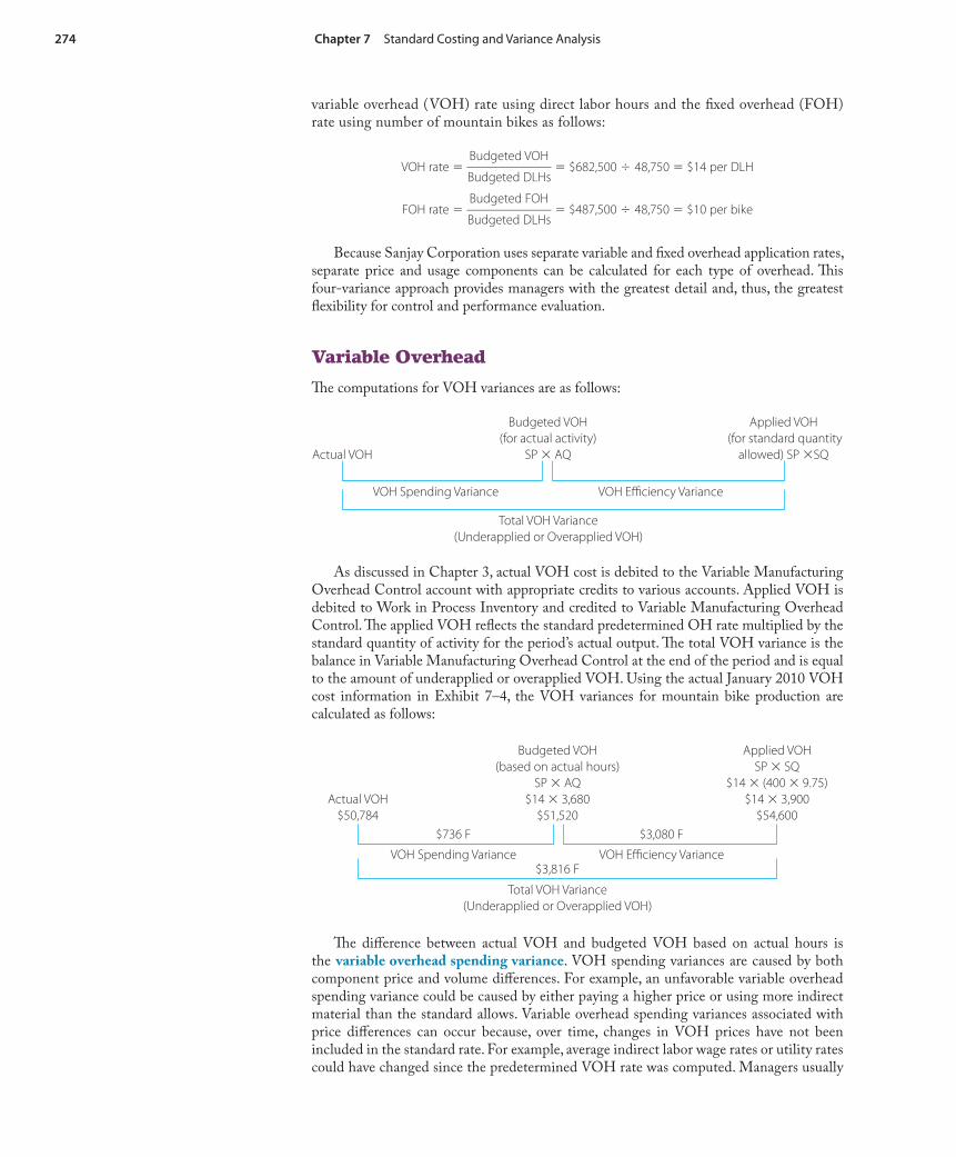
variable overhead (VOH) rate using direct labor hours and the fi xed overhead (FOH) rate using number of mountain bikes as follows:
VOH rate � Budgeted VOH
_____________ Budgeted DLHs
� $682,500 � 48,750 � $14 per DLH
FOH rate � Budgeted FOH
_____________ Budgeted DLHs
� $487,500 � 48,750 � $10 per bike
Because Sanjay Corporation uses separate variable and fi xed overhead application rates, separate price and usage components can be calculated for each type of overhead. Th is four-variance approach provides managers with the greatest detail and, thus, the greatest fl exibility for control and performance evaluation.
Variable Overhead
Th e computations for VOH variances are as follows:
As discussed in Chapter 3, actual VOH cost is debited to the Variable Manufacturing Overhead Control account with appropriate credits to various accounts. Applied VOH is debited to Work in Process Inventory and credited to Variable Manufacturing Overhead Control. Th e applied VOH refl ects the standard predetermined OH rate multiplied by the standard quantity of activity for the period’s actual output. Th e total VOH variance is the balance in Variable Manufacturing Overhead Control at the end of the period and is equal to the amount of underapplied or overapplied VOH. Using the actual January 2010 VOH cost information in Exhibit 7–4, the VOH variances for mountain bike production are calculated as follows:
Th e diff erence between actual VOH and budgeted VOH based on actual hours is the variable overhead spending variance. VOH spending variances are caused by both component price and volume diff erences. For example, an unfavorable variable overhead spending variance could be caused by either paying a higher price or using more indirect material than the standard allows. Variable overhead spending variances associated with price diff erences can occur because, over time, changes in VOH prices have not been included in the standard rate. For example, average indirect labor wage rates or utility rates could have changed since the predetermined VOH rate was computed. Managers usually
Actual VOH
Budgeted VOH (for actual activity)
SP � AQ
Applied VOH (for standard quantity
allowed) SP �SQ
VOH Spending Variance VOH Effi ciency Variance
Total VOH Variance(Underapplied or Overapplied VOH)
Actual VOH$50,784
Budgeted VOH (based on actual hours)
SP � AQ$14 � 3,680
$51,520
Applied VOHSP � SQ
$14 � (400 � 9.75)$14 � 3,900
$54,600$736 F $3,080 F
VOH Spending Variance VOH Effi ciency Variance$3,816 F
Total VOH Variance(Underapplied or Overapplied VOH)
Chapter 7 Standard Costing and Variance Analysis 275
have little control over prices charged by external parties and should not be held accountable for variances arising because of such price changes. In these instances, the standard rates should be adjusted.
Variable overhead spending variances associated with quantity diff erences can be caused by waste or shrinkage of production inputs (such as indirect material). For example, deterioration of material during storage or from lack of proper handling can be recognized only after the material is placed into production. Such occurrences usually have little relationship to the input activity basis used, but they do aff ect the VOH spending variance. If waste or spoil-age is the cause of the VOH spending variance, managers should be held accountable and encouraged to implement more eff ective controls.
Th e diff erence between budgeted VOH for actual hours and applied VOH is the variable overhead effi ciency variance. Th is variance quantifi es the eff ect of using more or less of the activity or resource that is the base for VOH application. For example, Sanjay Corporation applies VOH to mountain bikes using direct labor hours. If Sanjay uses direct labor time ineffi ciently, higher variable overhead costs will occur. When actual input exceeds standard input allowed, production operations are considered to be ineffi cient. Excess input also indicates that an increased VOH budget is needed to support the additional activity base being used.
Fixed Overhead
Th e total fi xed overhead (FOH) variance is divided into price and volume components by inserting budgeted FOH in the middle column of the general variance analysis model as follows:
Th e left column is the total actual fi xed overhead incurred. As discussed in Chapter 3, actual FOH cost is debited to Fixed Manufacturing Overhead Control and credited to vari-ous accounts. Budgeted FOH is a constant amount throughout the relevant range of activity and was the amount used to develop the predetermined FOH rate; thus, the middle column is a constant fi gure regardless of the actual quantity of input or the standard quantity of input
allowed.
Applied FOH is debited to Work in Process Inventory and credited to Fixed Manufacturing Overhead Control. Th e applied FOH refl ects the standard predeter-mined FOH rate multiplied by the standard quantity of activity for the period’s actual output. Th e total FOH variance is the balance in Fixed Manufacturing Overhead Control at the end of the period and is equal to the amount of underapplied or overap-plied FOH.
Total budgeted FOH for Sanjay Corporation for 2010 is given in Exhibit 7–3 as $487,500. Assuming that FOH is incurred steadily throughout the year, the monthly
Actual FOH Budgeted FOH
Applied FOH (for standard quantity allowed)
SP � SQ
FOH Spending Variance Volume Variance
Total FOH Variance(Underapplied or Overapplied FOH)
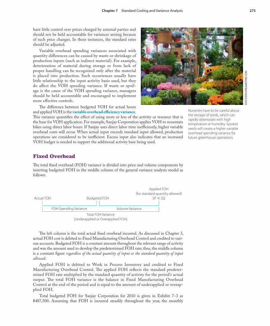
Nurseries have to be careful about the storage of seeds, which can rapidly deteriorate with high temperature or humidity. Spoiled seeds will create a higher variable overhead spending variance for future greenhouse operations.
GV
ICT
OR
IA/D
RE
AM
ST
IME
.CO
M
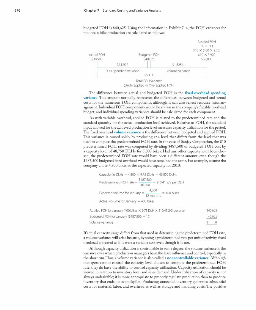
276 Chapter 7 Standard Costing and Variance Analysis
Th e diff erence between actual and budgeted FOH is the fi xed overhead spending variance. Th is amount normally represents the diff erences between budgeted and actual costs for the numerous FOH components, although it can also refl ect resource misman-agement. Individual FOH components would be shown in the company’s fl exible overhead budget, and individual spending variances should be calculated for each component.
As with variable overhead, applied FOH is related to the predetermined rate and the standard quantity for the actual production level achieved. Relative to FOH, the standard input allowed for the achieved production level measures capacity utilization for the period. Th e fi xed overhead volume variance is the diff erence between budgeted and applied FOH. Th is variance is caused solely by producing at a level that diff ers from the level that was used to compute the predetermined FOH rate. In the case of Sanjay Corporation, the $10 predetermined FOH rate was computed by dividing $487,500 of budgeted FOH cost by a capacity level of 48,750 DLHs for 5,000 bikes. Had any other capacity level been cho-sen, the predetermined FOH rate would have been a diff erent amount, even though the $487,500 budgeted fi xed overhead would have remained the same. For example, assume the company chose 4,800 bikes as the expected capacity for 2010:
Capacity in DLHs � 4,800 � 9.75 DLHs � 46,800 DLHs
Predetermined FOH rate � $487,500
________ 46,800
� $10.41 2/3 per DLH
Expected volume for January � 4,800
_________ 12 months
� 400 bikes
Actual volume for January � 400 bikes
Applied FOH for January (400 bikes � 9.75 DLH � $10.41 2/3 per bike) $40,625
Budgeted FOH for January ($487,500 � 12) 40,625
Volume variance $ 0
If actual capacity usage diff ers from that used in determining the predetermined FOH rate, a volume variance will arise because, by using a predetermined rate per unit of activity, fi xed overhead is treated as if it were a variable cost even though it is not.
Although capacity utilization is controllable to some degree, the volume variance is the variance over which production managers have the least infl uence and control, especially in the short run. Th us, a volume variance is also called a noncontrollable variance. Although managers cannot control the capacity level chosen to compute the predetermined FOH rate, they do have the ability to control capacity utilization. Capacity utilization should be viewed in relation to inventory level and sales demand. Underutilization of capacity is not always undesirable; it is more appropriate to properly regulate production than to produce inventory that ends up in stockpiles. Producing unneeded inventory generates substantial costs for material, labor, and overhead as well as storage and handling costs. Th e positive
budgeted FOH is $40,625. Using the information in Exhibit 7–4, the FOH variances for mountain bike production are calculated as follows:
Actual FOH$38,500
Budgeted FOH$40,625
Applied FOHSP � SQ
$10 � (400 � 9.75)$10 � 3,900
$39,000
$2,125 F $1,625 U
FOH Spending Variance Volume Variance$500 F
Total FOH Variance(Underapplied or Overapplied FOH)

Chapter 7 Standard Costing and Variance Analysis 277
impact that such unneeded production will have on the volume variance is insignifi cant because this variance is of little or no value for managerial control purposes.
Management is usually aware, as production occurs, of capacity utilization even if a volume variance is not reported. Th e volume variance merely translates under- or overuti-lization into a dollar amount. An unfavorable volume variance indicates less-than-expected utilization of capacity. If available capacity is commonly being used at a level higher (or lower) than that which was anticipated or is available, managers should recognize that condition, investigate the reasons for it, and (if possible and desirable) initiate appropriate action. Managers can infl uence capacity utilization by
modifying work schedules,•
taking measures to relieve any obstructions to or congestion of production activities,•
carefully monitoring the movement of resources through the production process, and•
acquiring needed, or disposing of unneeded, space and equipment.•
Preferably, such actions should be taken before production rather than after it. Eff orts made after production is completed might improve next period’s operations but will have no impact on past production.
Alternative Overhead Variance Approaches
If the accounting system does not separate variable and fi xed overhead costs, insuffi cient data will be available to compute four overhead variances. Use of a combined (variable and fi xed) predetermined OH rate requires alternative overhead variance computations. One approach is to calculate only the total overhead variance, which is the diff erence between total actual overhead and total overhead applied to production. Th e amount of applied overhead is found by multiplying the combined rate by the standard quantity allowed for the actual production. Th e one-variance approach is as follows:
Actual OverheadVariable OH � Fixed OH
Applied OverheadSP � SQ
Like other total variances, the total overhead variance provides limited information to managers. For Sanjay Corporation, the total overhead variance is calculated as follows:
Actual OverheadVOH + FOH
$50,784 � $38,500$89,284
Applied OverheadSP � SQ
$24 � 3,900$93,600
Note that this amount is the same as the summation of the $3,816 F total VOH variance and the $500 F total FOH variance computed under the four-variance approach.
A two-variance analysis is performed by inserting a middle column in the one-variance model:
Total Overhead Variance
Total Overhead Variance
Actual OverheadVOH + FOH
Budgeted Overhead (for standard quantity)
Applied Overhead SP � SQ
Budget Variance (or Controllable Variance)
Volume Variance (or Noncontrollable Variance)
Total Overhead Variance
$4,316 F
278 Chapter 7 Standard Costing and Variance Analysis
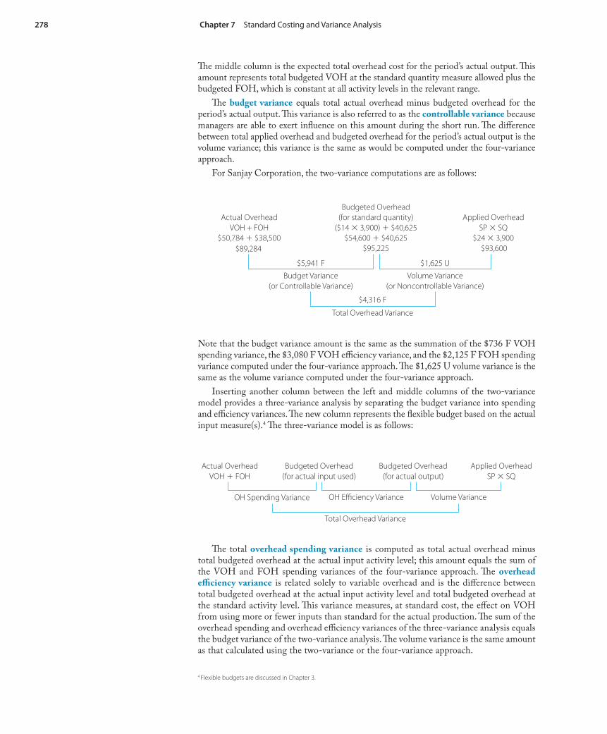
Th e middle column is the expected total overhead cost for the period’s actual output. Th is amount represents total budgeted VOH at the standard quantity measure allowed plus the budgeted FOH, which is constant at all activity levels in the relevant range.
Th e budget variance equals total actual overhead minus budgeted overhead for the period’s actual output. Th is variance is also referred to as the controllable variance because managers are able to exert infl uence on this amount during the short run. Th e diff erence between total applied overhead and budgeted overhead for the period’s actual output is the volume variance; this variance is the same as would be computed under the four-variance approach.
For Sanjay Corporation, the two-variance computations are as follows:
Note that the budget variance amount is the same as the summation of the $736 F VOH spending variance, the $3,080 F VOH effi ciency variance, and the $2,125 F FOH spending variance computed under the four-variance approach. Th e $1,625 U volume variance is the same as the volume variance computed under the four-variance approach.
Inserting another column between the left and middle columns of the two-variance model provides a three-variance analysis by separating the budget variance into spending and effi ciency variances. Th e new column represents the fl exible budget based on the actual input measure(s).4 Th e three-variance model is as follows:
Th e total overhead spending variance is computed as total actual overhead minus total budgeted overhead at the actual input activity level; this amount equals the sum of the VOH and FOH spending variances of the four-variance approach. Th e overhead effi ciency variance is related solely to variable overhead and is the diff erence between total budgeted overhead at the actual input activity level and total budgeted overhead at the standard activity level. Th is variance measures, at standard cost, the eff ect on VOH from using more or fewer inputs than standard for the actual production. Th e sum of the overhead spending and overhead effi ciency variances of the three-variance analysis equals the budget variance of the two-variance analysis. Th e volume variance is the same amount as that calculated using the two-variance or the four-variance approach.
4 Flexible budgets are discussed in Chapter 3.
Actual OverheadVOH + FOH
$50,784 � $38,500
Budgeted Overhead (for standard quantity)
($14 � 3,900) � $40,625$54,600 � $40,625
Applied OverheadSP � SQ
$24 � 3,900
$5,941 FBudget Variance
(or Controllable Variance)Volume Variance
(or Noncontrollable Variance)
$4,316 F
Total Overhead Variance
$89,284 $95,225 $93,600
$1,625 U
Total Overhead Variance
Actual OverheadVOH � FOH
Budgeted Overhead (for actual input used)
Budgeted Overhead (for actual output)
Applied OverheadSP � SQ
OH Spending Variance OH Effi ciency Variance Volume Variance

Chapter 7 Standard Costing and Variance Analysis 279
For Sanjay Corporation, the three-variance computations are as follows:
Actual OverheadVOH � FOH
$50,784 � $38,500
Budgeted Overhead (for actual input)
($14 � 3,680) � $40,625$51,520 � $40,625
Budgeted Overhead (for actual output)
($14 � 3,900) � $40,625$54,600 � $40,625
Applied OverheadSP � SQ
$24 � 3,900
$2,861 F
OH Spending Variance OH Effi ciency Variance Volume Variance
$4,316 F
Total Overhead Variance
$89,284 $92,145
$3,080 F
$95,225 $93,600
$1,625 U
Note that the OH spending variance amount is the same as the summation of the $736 F VOH spending variance and the $2,125 F FOH spending variance computed under the four-variance approach. Th e $3,080 F OH effi ciency variance is the same as the VOH effi ciency variance computed under the four-variance approach, and the $1,625 U volume variance is the same as the volume variance computed under the four-variance approach.
If VOH and FOH are applied using a combined rate, the one-, two-, and three-vari-ance approaches will have the interrelationships shown in Exhibit 7–5. Th e amounts in the exhibit represent the data provided earlier for Sanjay Corporation. Managers should select the method that provides the most useful information and that conforms to the company’s accounting system. As more companies begin to recognize the existence of multiple cost drivers for overhead and to use multiple bases for applying overhead to production, compu-tation of the one-, two-, and three-variance approaches will diminish.
Standard Cost System Journal EntriesSanjay Corporation’s January 2010 journal entries for mountain bike production are shown in Exhibit 7–6 (p. 280). Th e following explanations apply to the numbered journal entries:
1. Th e debit to Raw Material Inventory is for the standard price of the actual quantity of component WF-05 purchased in January. Th e credit to Accounts Payable is for the actual price of the actual quantity of component WF-05 purchased. Th e variance credit refl ects the favorable material price variance for that component. Similar entries would be made for purchases of all other components.
2. Th e debit to Work in Process Inventory is for the standard price of the standard quan-tity of the WF-05 component used in January; the Raw Material Inventory credit is
Exhibit 7–5 Interrelationships of Overhead Variances
Four Variance
VOH Variances: Spending $ 736 F Efficiency $3,080 F
FOH Variances: Spending $2,125 F Volume $1,625 U
Three Variance
Spending $2,861 F Efficiency $3,080 F Volume $1,625 U
Two Variance
$5,941 F
Budget (Controllable) Volume $1,625 U
One Variance
$4,316 F
Total Overhead Variance

280 Chapter 7 Standard Costing and Variance Analysis
for the standard price of the actual quantity of WF-05 components used in production. Th e debit to the Material Quantity Variance account refl ects the overuse (by 13 units) of WF-05s, valued at the standard price. Similar entries would be made for issuances of all other components to production.
3. Th e debit to Work in Process Inventory is for the standard hours in the Painting Department to produce 400 mountain bikes multiplied by the standard wage rate. Th e Wages Payable credit is for the actual amount of direct cost for painters during the period. Th e Labor Effi ciency Variance credit refl ects the diff erence between actual and standard hours multiplied by the standard wage rate. Similar entries would be made for wages incurred and standard direct labor wages allowed for all other departments.
4. During January, actual costs incurred for variable and fi xed overhead are debited to the Manufacturing Overhead Control accounts. Th ese costs are caused by a variety of
Exhibit 7–6 Selected Journal Entries for Sanjay Corporation’s Mountain Bike Production, January 2010
(1) Raw Material Inventory ($20 � 450) 9,000
Material Purchase Price Variance [($20 � $19) � 450] 450
Accounts Payable 8,550
To record the acquisition of 450 WF-05s
(2) Work in Process Inventory ($20 � 400 � 1) 8,000
Material Quantity Variance {$20 � [(400 � 1) � 413]} 260
Raw Material Inventory ($20 � 413) 8,260
To record issuance of WF-05s to production
(3) Work in Process Inventory [$12 � (400 � 3)] 14,400
Labor Rate Variance [($12 � $12) � 1,100] 0
Labor Effi ciency Variance {$12 � [(400 � 3) � 1,100]} 1,200
Wages Payable ($12 � 1,100) 13,200
To record incurrence of direct labor costs by the Painting Department (Note: In an actual organization, no journal entry debit would have
been made for the labor rate variance because the amount was $0.)
(4) Variable Manufacturing Overhead Control 50,784
Fixed Manufacturing Overhead Control 38,500
Various accounts 89,284
To record actual overhead costs
(5) Work in Process Inventory 93,600
Variable Manufacturing Overhead Control ($14 � 400 � 9.75) 54,600
Fixed Manufacturing Overhead Control ($10 � 400 � 9.75) 39,000
To apply predetermined overhead to the month’s production
(6) Variable Manufacturing Overhead Control ($54,600 � $50,784) 3,816
Variable Overhead Spending Variance 736
Variable Overhead Effi ciency Variance 3,080
To close variable OH and recognize the variable OH variances
(7) Volume Variance [($10 � 400 � 9.75) � ($487,500 � 12)] 1,625
Fixed Manufacturing Overhead Control ($39,000 � $38,500) 500
Fixed Overhead Spending Variance [$38,500 � ($487,500 � 12)] 2,125
To close fi xed OH and recognize the fi xed OH variances

Chapter 7 Standard Costing and Variance Analysis 281
transactions including indirect material and labor usage, depreciation, and utility costs. Th is entry refl ects the incurrence of all company overhead for the month.
5. Overhead is applied to production using the predetermined rates multiplied by the standard input allowed. Overhead application is recorded at completion of production or at the end of the period, whichever occurs fi rst. Th e diff erence between actual debits and applied credits in each overhead account represents the total variable and fi xed overhead variances and is also the underapplied or overapplied overhead for the period. For January, variable overhead and fi xed overhead are applied at the respective $14 per DLH and $10 per DLH predetermined rates.
6. & 7. Th ese entries assume an end-of-month closing of the Variable Manufacturing Overhead Control and Fixed Manufacturing Overhead Control accounts. Th ese entries close the manufacturing overhead accounts and recognize the overhead variances. Th e balances in the accounts are reclassifi ed to the appropriate variance accounts. Th is entry is provided for illustration only. Th is process would typically not be performed at month-end but rather at year-end because an annual period was used to calculate the predetermined OH rates.
Note that all unfavorable variances have debit balances and favorable variances have credit balances. Unfavorable variances represent excess production costs; favorable vari-ances represent savings in production costs. Standard production costs are shown in inven-tory accounts (which have debit balances); therefore, excess costs are also debits.
Although standard costs are useful for internal reporting, they can be used in fi nan-cial statements only if the amounts are substantially equivalent to those that would have resulted from using an actual cost system. If standards are achievable and current, this equivalency should exist. Standard costs in fi nancial statements should provide fairly con-servative inventory valuations because the eff ects of excess price and/or ineffi cient opera-tions are eliminated.
At year-end, adjusting entries are made to eliminate standard cost variances. Th e entries depend on whether the variances are, in total, insignifi cant or signifi cant. If the combined impact of the variances is insignifi cant, unfavorable variances are closed as debits to Cost of Goods Sold; favorable variances are credited to Cost of Goods Sold. Th us, unfavorable variances decrease operating income because of the higher-than-expected costs whereas favorable variances increase operating income because of the lower-than-expected costs. Even if the year’s entire production has not been sold yet, this variance treatment is based on the immateriality of the amounts involved.
In contrast, large variances are prorated at year-end among ending inventories and Cost of Goods Sold so that the balances in those accounts approximate actual costs. Proration is based on the relative size of the account balances. Disposition of signifi cant variances is similar to the disposition of large amounts of underapplied or overapplied overhead as shown in Chapter 3.
To illustrate the disposition of signifi cant variances, assume that Nailz Company has a $20,000 unfavorable (debit) year-end Material Purchase Price Variance. Th e company considers this amount signifi cant. Nailz makes one type of product, which requires a single raw material input. Other relevant year-end account balances for Nailz Company are as follows:
Raw Material Inventory $ 49,126
Work in Process Inventory 28,072
Finished Goods Inventory 70,180
Cost of Goods Sold 554,422
Total of aff ected accounts $701,800
Th e theoretically correct allocation of the material price variance would use actual mate-rial cost in each account at year-end. However, as was mentioned in Chapter 3 with regard to overhead, after the conversion process has begun, cost elements within account balances are commingled and tend to lose their identity. Th us, unless a signifi cant misstatement

282 Chapter 7 Standard Costing and Variance Analysis
LO.3 Why are standard cost systems used?
would result, disposition of the variance can be based on the proportions of each account balance to the total, as follows:
Raw Material Inventory 7% ($49,126 � $701,800)
Work in Process Inventory 4 ($28,072 � $701,800)
Finished Goods Inventory 10 ($70,180 � $701,800)
Cost of Goods Sold 79 ($554,422 � $701,800)
Total 100%
Applying these percentages to the $20,000 material purchase price variance gives the amounts in the following journal entry to assign to the aff ected accounts:
Raw Material Inventory ($20,000 � 0.07) 1,400
Work in Process Inventory ($20,000 � 0.04) 800
Finished Goods Inventory ($20,000 � 0.10) 2,000
Cost of Goods Sold ($20,000 � 0.79) 15,800
Material Purchase Price Variance 20,000
To dispose of the material purchase price variance at year-end
All variances other than the material price variance occur as part of the conversion pro-cess. Because conversion includes raw material put into production (rather than raw mate-rial purchased), all remaining variances are prorated only to Work in Process Inventory, Finished Goods Inventory, and Cost of Goods Sold.
Th e preceding discussion about standard setting, variance computations, and year-end adjustments indicates that a substantial commitment of time and eff ort is required to implement and use a standard cost system. Companies are willing to make such a commit-ment for a variety of reasons.
Why Standard Cost Systems Are UsedStandard cost systems require less clerical time and eff ort than are necessary in an actual cost system. A standard cost system assigns costs to inventory and Cost of Goods Sold accounts at predetermined amounts per unit regardless of actual conditions. With an actual cost system, actual unit costs change continuously with changes in prices and usage of inputs. A standard cost system holds unit costs constant for some period. However, more importantly than the clerical effi ciency provided, standard cost systems are designed to provide information for managers to use in performing their various functions.
Motivating
Standards help communicate management’s expectations to workers. When standards are achievable and rewards for attaining them are available, workers are likely to be motivated to strive to meet them. Th e attainment of standards, however, must require a reasonable amount of eff ort on the workers’ part.
Planning
Financial and operational planning requires estimates about future prices and usage of inputs. Managers can use current standards to estimate future quantity needs and costs. Th ese estimates help determine purchasing needs for material, staffi ng needs for labor, and capacity needs related to overhead and planning for company cash fl ows. In addition, use of a standard simplifi es budget preparation because a standard is, in fact, a budget for one unit of product or service. Standards are also used to provide the cost basis needed to analyze relationships among the organization’s costs, sales volume, and profi ts.

Chapter 7 Standard Costing and Variance Analysis 283
Controlling
Th e control process begins with the establishment of standards as a basis against which actual costs can be measured and variances calculated. Variance analysis is the process of categorizing the nature (favorable or unfavorable) of the diff erences between actual and standard costs and seeking explanations for those diff erences. A well-designed variance analysis system computes variances as early as possible subject to cost–benefi t assessments. Th e system should help managers determine who or what was responsible for each vari-ance and who is best able to explain it. An early measurement and reporting system allows managers to quickly monitor operations and take corrective action if necessary.
In analyzing variances, managers must recognize that they have a specifi c scarce resource: their time. Th ey must distinguish between situations that can be ignored and those that need attention. To do this, managers establish upper and lower tolerance limits of accept-able deviations from the standard. If variances are small and within an acceptable range, no managerial action is required. If a variance diff ers signifi cantly from standard, the manager responsible for the cost is expected to identify the variance cause(s) and then take actions to eliminate future unfavorable variances or, perhaps, to perpetuate favorable variances.
Setting upper and lower tolerance limits for deviations (as illustrated in Exhibit 7–7) allows managers to implement the management-by-exception concept. In the exhibit, the only signifi cant deviation from standard occurred on Day 5, when the actual cost exceeded the upper limit of acceptable performance. An exception report should be gen-erated on this date so that the manager can investigate the underlying variance causes.
Exhibit 7–7 Illustration of Management-by-Exception Concept
1 2 3 4 5 6Day of Week
Dol
lars
of C
ost Acceptable
upper limit
Acceptablelower limit
Standard Unit Cost
Within acceptable range
Outside acceptable range
Variances large enough to fall outside the acceptability ranges often indicate prob-lems. However, a mere computation of a variance does not reveal the variance’s cause nor the person or group responsible for it. To determine variance causality, managers must investigate signifi cant variances through observation, inspection, and inquiry. Th e investi-gation involves people at the operating level as well as accounting personnel. Operations personnel should spot variances as they occur and record the reasons for the variances to the extent that those reasons are discernible. For example, operating personnel could readily detect and report causes such as machine downtime or material spoilage.
One important point about variances must be made: favorable variance is not neces-sarily a good variance. Although people often equate “favorable” with “good,” an extremely favorable variance could mean that an error was made when the standard was set or that

284 Chapter 7 Standard Costing and Variance Analysis
a related, off setting unfavorable variance exists. For example, if low-grade material is pur-chased, a favorable price variance may result, but additional material might have to be used to overcome defective production. Also, an unfavorable labor effi ciency variance might result because more time was required to complete a job as a result of using the inferior material. Another common situation begins with labor rather than material. Using workers who are lower paid but less skilled than others will result in a favorable rate variance but can cause excessive use of raw material and of labor time. Managers must be aware that such relationships exist and that variances cannot be analyzed in isolation.
Variance computations are being made more often than in the past. Monthly variance reporting is still common, but there is movement toward shorter reporting periods. As more companies integrate total quality management and just-in-time production into their opera-tions, variance reporting and analysis will become more frequent.5 Additionally, standards should defi nitely be updated as an organization implements changes in production technology.
Decision Making
Standard cost information facilitates decision making. For example, managers can compare a standard cost with a quoted price to determine whether an item should be manufactured in-house or purchased. Using actual cost information in such a decision could be inappropriate because the actual cost could fl uctuate each period. Also, in deciding whether to off er a special price to customers, managers can use standard product cost to determine the lowest price limit. Similarly, a company bidding on contracts must have some idea of estimated product costs. Bidding too low and winning the contract could cause substantial operating income (and, possibly, cash fl ow) reduction bidding too high could be noncompetitive and cause the contract to be awarded to another company.
Performance Evaluation
Variance reports should be analyzed for both positive and negative information as soon as they are received. Management needs to know when costs were and were not controlled and who is responsible. Such information allows management to provide feedback to subordinates, investigate areas of concern, and make performance evaluations about who needs additional supervision, who should be replaced, and who should be promoted. For proper performance evaluations to be made, variance responsibility must be traced to specifi c managers.6
Considerations in Establishing StandardsWhen standards are established, the issues of appropriateness and attainability should be con-sidered. Appropriateness, in relation to a standard, refers to the bases on which the standards are developed and how long they will be viable. Attainability refers to management’s belief about the degree of diffi culty or rigor that should be exerted in achieving the standard.
Appropriateness
Although developed from past and current information, standards must evolve to refl ect relevant future technical and environmental factors. Consideration should be given to fac-tors such as material quality, normal material-ordering quantities, expected employee wage rates, mix of employee skills, facility layout, and expected degree of plant automation. Once set, standards will not remain useful forever. Current operating performance should not be compared to out-of-date standards because such comparisons will generate variances that are not logical bases for planning, controlling, decision making, or performance evaluation.
5 Total quality management is discussed in Chapter 17, and just-in-time production is discussed in Chapter 18.6 Responsibility accounting, performance evaluation, and cost control relative to variances are discussed in greater depth in, respectively, Chapters 13, 14, and 16.
Chapter 7 Standard Costing and Variance Analysis 285
LO.4 How have the setting and use of standards changed over time?
Attainability
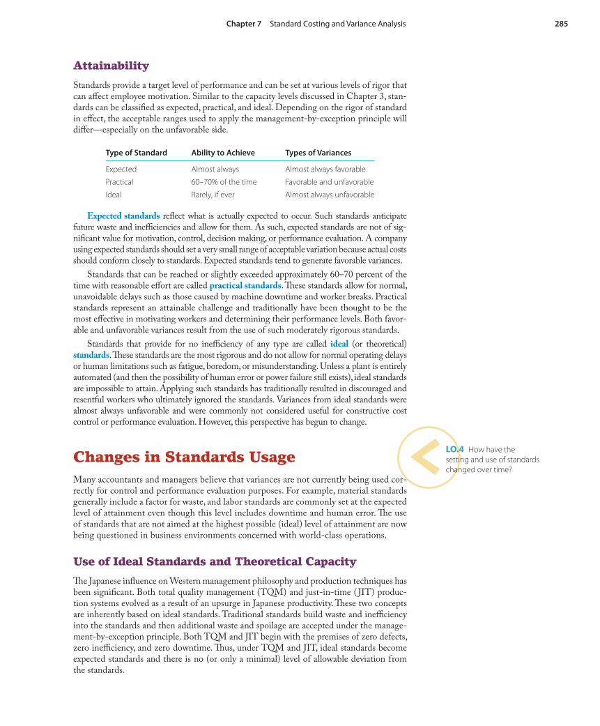
Standards provide a target level of performance and can be set at various levels of rigor that can aff ect employee motivation. Similar to the capacity levels discussed in Chapter 3, stan-dards can be classifi ed as expected, practical, and ideal. Depending on the rigor of standard in eff ect, the acceptable ranges used to apply the management-by-exception principle will diff er—especially on the unfavorable side.
Type of Standard Ability to Achieve Types of Variances
Expected Almost always Almost always favorable
Practical 60–70% of the time Favorable and unfavorable
Ideal Rarely, if ever Almost always unfavorable
Expected standards refl ect what is actually expected to occur. Such standards anticipate future waste and ineffi ciencies and allow for them. As such, expected standards are not of sig-nifi cant value for motivation, control, decision making, or performance evaluation. A company using expected standards should set a very small range of acceptable variation because actual costs should conform closely to standards. Expected standards tend to generate favorable variances.
Standards that can be reached or slightly exceeded approximately 60–70 percent of the time with reasonable eff ort are called practical standards. Th ese standards allow for normal, unavoidable delays such as those caused by machine downtime and worker breaks. Practical standards represent an attainable challenge and traditionally have been thought to be the most eff ective in motivating workers and determining their performance levels. Both favor-able and unfavorable variances result from the use of such moderately rigorous standards.
Standards that provide for no ineffi ciency of any type are called ideal (or theoretical) standards. Th ese standards are the most rigorous and do not allow for normal operating delays or human limitations such as fatigue, boredom, or misunderstanding. Unless a plant is entirely automated (and then the possibility of human error or power failure still exists), ideal standards are impossible to attain. Applying such standards has traditionally resulted in discouraged and resentful workers who ultimately ignored the standards. Variances from ideal standards were almost always unfavorable and were commonly not considered useful for constructive cost control or performance evaluation. However, this perspective has begun to change.
Changes in Standards UsageMany accountants and managers believe that variances are not currently being used cor-rectly for control and performance evaluation purposes. For example, material standards generally include a factor for waste, and labor standards are commonly set at the expected level of attainment even though this level includes downtime and human error. Th e use of standards that are not aimed at the highest possible (ideal) level of attainment are now being questioned in business environments concerned with world-class operations.
Use of Ideal Standards and Theoretical Capacity
Th e Japanese infl uence on Western management philosophy and production techniques has been signifi cant. Both total quality management (TQM) and just-in-time ( JIT) produc-tion systems evolved as a result of an upsurge in Japanese productivity. Th ese two concepts are inherently based on ideal standards. Traditional standards build waste and ineffi ciency into the standards and then additional waste and spoilage are accepted under the manage-ment-by-exception principle. Both TQM and JIT begin with the premises of zero defects, zero ineffi ciency, and zero downtime. Th us, under TQM and JIT, ideal standards become expected standards and there is no (or only a minimal) level of allowable deviation from the standards.
286 Chapter 7 Standard Costing and Variance Analysis
Workers may, at fi rst, resent the introduction of standards set at a “perfection” level, but it is in their own and management’s best long-run interest to have such standards for the following reasons.
When a standard is set at a less-than-ideal level, managers are allowing and encouraging • ineffi cient resource utilization.
If no ineffi ciencies are built into or tolerated in the system, deviations from standard • should be minimized and overall organizational performance improved.
Higher standards for effi ciency automatically mean lower costs because of the elimination • of non-value-added activities such as waste, idle time, and rework.
Ideal standards require that employees communicate and work together to improve • performance.
Ideal standards result in the most useful information for managerial purposes as well as • the highest-quality products and services at the lowest possible cost.
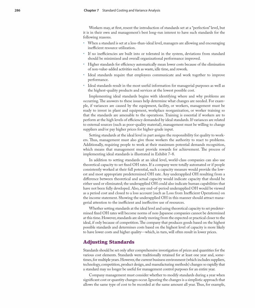
Implementing ideal standards begins with identifying where and why problems are occurring. Th e answers to these issues help determine what changes are needed. For exam-ple, if variances are caused by the equipment, facility, or workers, management must be ready to invest in plant and equipment, workplace reorganization, or worker training so that the standards are amenable to the operations. Training is essential if workers are to perform at the high levels of effi ciency demanded by ideal standards. If variances are related to external sources (such as poor-quality material), management must be willing to change suppliers and/or pay higher prices for higher-grade input.
Setting standards at the ideal level in part assigns the responsibility for quality to work-ers. Th us, management must also give those workers the authority to react to problems. Additionally, requiring people to work at their maximum potential demands recognition, which means that management must provide rewards for achievement. Th e process of implementing ideal standards is illustrated in Exhibit 7–8.
In addition to setting standards at an ideal level, world-class companies can also use theoretical capacity to set fi xed OH rates. If a company were totally automated or if people consistently worked at their full potential, such a capacity measure would provide the low-est and most appropriate predetermined OH rate. Any underapplied OH resulting from a diff erence between theoretical and actual capacity would indicate capacity that should be either used or eliminated; the underapplied OH could also indicate human capabilities that have not been fully developed. Also, any end-of-period underapplied OH would be viewed as a period cost and closed to a loss account (such as Loss from Ineffi cient Operations) on the income statement. Showing the underapplied OH in this manner should attract mana-gerial attention to the ineffi cient and ineff ective use of resources.
Whether setting standards at the ideal level and using theoretical capacity to set predeter-mined fi xed OH rates will become norms of non-Japanese companies cannot be determined at this time. However, standards are slowly moving from the expected or practical closer to the ideal, if only because of competition. Th e company that produces goods based on the highest possible standards and determines costs based on the highest level of capacity is more likely to have lower costs and higher quality—which, in turn, will often result in lower prices.
Adjusting Standards
Standards should be set only after comprehensive investigation of prices and quantities for the various cost elements. Standards were traditionally retained for at least one year and, some-times, for multiple years. However, the current business environment (which includes suppliers, technology, competition, product design, and manufacturing methods) changes so rapidly that a standard may no longer be useful for management control purposes for an entire year.
Company management must consider whether to modify standards during a year when signifi cant cost or quantity changes occur. Ignoring the changes is a simplistic approach that allows the same type of cost to be recorded at the same amount all year. Th us, for example,
Chapter 7 Standard Costing and Variance Analysis 287
any material purchased during the year would be recorded at the same standard cost regard-less of when it was purchased. Although making recordkeeping easy, this approach elimi-nates any opportunity to adequately control costs or evaluate performance. Additionally, such an approach could create large diff erentials between standard and actual costs, making standard costs unacceptable for external reporting.
Adjusting standards to refl ect price or quantity changes would make some aspects of management control and performance evaluation more eff ective, and others more diffi cult. For instance, budgets prepared using the original standards would need to be adjusted before appropriate actual comparisons could be made against them. Changing standards also cre-ates a problem for recordkeeping and inventory valuation. Accountants would have to decide whether products should be valued at the standard cost that was in eff ect when they were made or at the standard cost in eff ect when the fi nancial statements were prepared. Although production-point standards would be more closely related to actual costs, the use of such standards might undermine many of the benefi ts discussed earlier in the chapter.
If possible, management should consider combining these two choices in the accounting system. Th e original standards can be considered “frozen” for budget purposes and a revised budget can be prepared using the new current standards. Diff erences between these two bud-gets would refl ect variances related to business environment cost changes. Th ese variances could be designated as uncontrollable (such as those related to changes in the market price of raw material) or internally initiated (such as changes in standard labor time resulting from employee training or equipment rearrangement). Comparing the budget based on current stan-dards with actual costs incurred would provide variances that more adequately refl ect internally
Exhibit 7–8 Implementing Ideal Standards
Set ideal standards and communicate reasoning to workers
Make necessarychanges in materialquality or vendors
Give workers theauthority and respon-
sibility to react toproblems
Identify where andwhy variances are
occurring
Make necessary in-vestments in plant andequipment, workplace
reorganization, orworker training
Provide appropriaterecognition and re-
wards to workers
Achieveworld-class
competitive-ness
Achieveworld-class
competitive-ness
Assess ways to con-tinuously improveoperations and re-evaluate standards

288 Chapter 7 Standard Costing and Variance Analysis
LO.5 How does the use of a single conversion element (rather than the traditional labor and overhead elements) aff ect standard costing?
Exhibit 7–9 Combined “Frozen” and Revised Budget System for Variance Analysis
Budget—original standards
Budget—current standards
Variances related tobusiness environment
Internally Initiated
Controllable
Actual prices andquantities
Variances related to inter-nally controllable causes
Uncontrollable
controllable causes, such as excess material and/or labor time usage caused by inferior material purchases. A combined “frozen” and revised budget system is depicted in Exhibit 7–9.
Material Price Variance Based on Usage Rather Than on Purchases
Th e material price variance computation has traditionally been based on purchases rather than on usage to calculate the variance as quickly as possible relative to the cost incurrence. Although calculating the material price variance at purchase point allows managers to see the impact of buying decisions rapidly, such information might not be most relevant in a JIT environment. Buying material that is not needed for current production requires that the material be stored and moved, both of which are non-value-added activities. Th e trade-off in price savings should be measured against the additional costs to determine the cost–benefi t relationship of such a purchase.
Additionally, computing a material price variance on purchases rather than on usage can reduce the probability of recognizing a relationship between a favorable material price variance and an unfavorable material quantity variance. If a favorable price variance resulted from buying low-grade material, the potential negative eff ects of that purchase on material usage and labor effi ciency will not be known until the material is actually used.
Decline in Direct Labor
As the proportion of product cost comprised of direct labor declines, the necessity for direct labor variance computations is minimized. Automation often relegates labor to an indi-rect category because workers become machine overseers rather than producers of goods. Accordingly, direct labor can be combined with overhead to become viewed as the “conver-sion cost” of a product.
Conversion Cost as an Element in Standard CostingAs discussed in Chapter 2, conversion cost consists of direct labor and manufacturing over-head. Th e traditional view of separating product cost into three categories (direct material, direct labor, and overhead) is appropriate in a labor-intensive production setting. However, in automated factories, direct labor cost often represents only a small part of total product cost. In such circumstances, one worker might oversee a large number of machines and deal more with troubleshooting machine malfunctions than with converting raw material into fi nished products. Th ese new conditions mean that workers are probably considered indi-rect rather than direct labor and, therefore, their wages should be considered overhead.

Chapter 7 Standard Costing and Variance Analysis 289
Many automated companies have adapted their standard cost systems to provide for only two elements of product cost: direct material and conversion. In these situations, conversion cost is likely to be separated into variable and fi xed components. Conversion cost can also be separated into direct and indirect categories based on the ability to trace such costs to a machine rather than to a product. Overhead can be applied under an activity-based costing methodology (see Chapter 4) using a variety of cost drivers such as number of machine hours, material cost, number of production runs, number of machine setups, or throughput time.
Variance analysis for conversion cost in automated plants normally focuses on the following:
spending variances for overhead costs,•
effi ciency variances for machinery and production costs rather than labor costs, and•
a volume variance for production.•
Th ese analyses are similar to the traditional three-variance overhead approach. In an auto-mated system, managers are better able to control not only the spending and effi ciency variances but also the volume variance. Th e idea of planned output is essential in a JIT system. Variance analysis under a conversion cost approach is illustrated in Exhibit 7–10. Regardless of how variances are computed, managers must analyze those variances and use them for cost control purposes to the extent that such control can be exercised.
Assume that Christopher Corp. makes bike frames in a fully automated production facility; all labor required for this product is considered indirect. For simplicity, it is assumed
Variable Conversion Rate �Standard Machine Hours Allowed
Exhibit 7–10 Variances under Conversion Approach
Conversion Rate per MH* � Budgeted Direct Labor Cost � Budgeted OH Cost
________________________________________ Budgeted Machine Hours
(can be separated into variable and fi xed costs)
If variable and fi xed conversion costs are separated:
If variable and fi xed overhead are not separated:
*Other cost drivers could be more appropriate than MHs. If such drivers are used to determine the rate, they must also be used to determine the variances.
VolumeVariance
Total Fixed Conversion Variance
Fixed ConversionSpending Variance
Actual FixedConversion Cost
Budgeted FixedConversion Cost
Fixed Conversion Rate �Standard Machine Hours Allowed
Actual Variable Conversion Cost
Variable Conversion Rate� Actual Machine Hours
Variable ConversionEffi ciency Variance
Total Variable Conversion Variance
Variable ConversionSpending Variance
Flexible Budgetfor Actual
Machine Hours
Flexible Budgetfor Standard Machine
Hours Allowed
Conversion Rate � Standard Machine
Hours AllowedActual
Conversion Costs
Spending Variance Volume Variance
Total Conversion Variance
Effi ciency Variance

290 Chapter 7 Standard Costing and Variance Analysis
LO.6 How are variances aff ected by multiple material and labor categories?
that all overhead is applied on the basis of budgeted machine hours. Necessary 2010 pro-duction and cost information for bike frames is as follows:
Expected production 48,000 units
Actual production 50,000 units
Actual machine time 37,100 MHs
Standard machine time allowed per unit .75 MH
Budgeted variable conversion cost $144,000
Budgeted fi xed conversion cost $306,000
Actual variable conversion cost $150,500
Actual fi xed conversion cost $304,600
Variable conversion rate: $144,000 � 36,000 MHs � $4.00 per MH
Fixed conversion rate: $306,000 � 36,000 � $8.50 per MH
Standard machine hours allowed: 50,000 units � 0.75 hour per unit � 37,500 MHs
Th e three-variance computations for conversion costs follow.
Flexible Budget at Standard Hours
[($4 � 37,500) � $306,000]$456,000
Standard Cost ($12.50 � 37,500)
$468,750
$1,600 FEffi ciencyVariance
$12,750 FVolumeVariance
Flexible Budget at Actual Hours
[($4 � 37,100) � $306,000]$454,400
Actual Conversion Cost
($150,200 � $304,600)$455,100
$700 USpending Variance
$13,650 F
Total Conversion Cost Variance
Th e spending variance could be divided into a $1,800 U variable overhead spending vari-ance and a $1,400 F fi xed overhead spending variances as follows:
VOH spending variance � $150,200 � ($4 � $37,100) � $150,200 � $148,400 � $1,800 U
FOH spending variance � $304,600 � $306,000 � �$1,400 F
Appendix
Mix and Yield VariancesMost companies combine many materials and various classes of direct labor to produce goods. In such settings, the material and labor variance computations presented in this chapter are insuffi cient.
When a product is made from multiple materials, a goal is to combine the materials in a way that produces the desired quality in the most cost-benefi cial manner. Sometimes materials can be substituted for one another without aff ecting product quality. In other instances, only one specifi c material or type of material can be used. For example, a furniture manufacturer might use either oak or maple to build a couch frame and still have the same basic quality. However, a perfume manufacturer might have to use a very specifi c fragrance oil to achieve a desired scent.
Labor, like materials, can be combined in many diff erent ways to make the same prod-uct. Some combinations are less expensive or more effi cient than others. As with materi-als, some degree of interchangeability between labor categories is assumed. However, all potential combinations could not be viable; for example, unskilled workers could not be
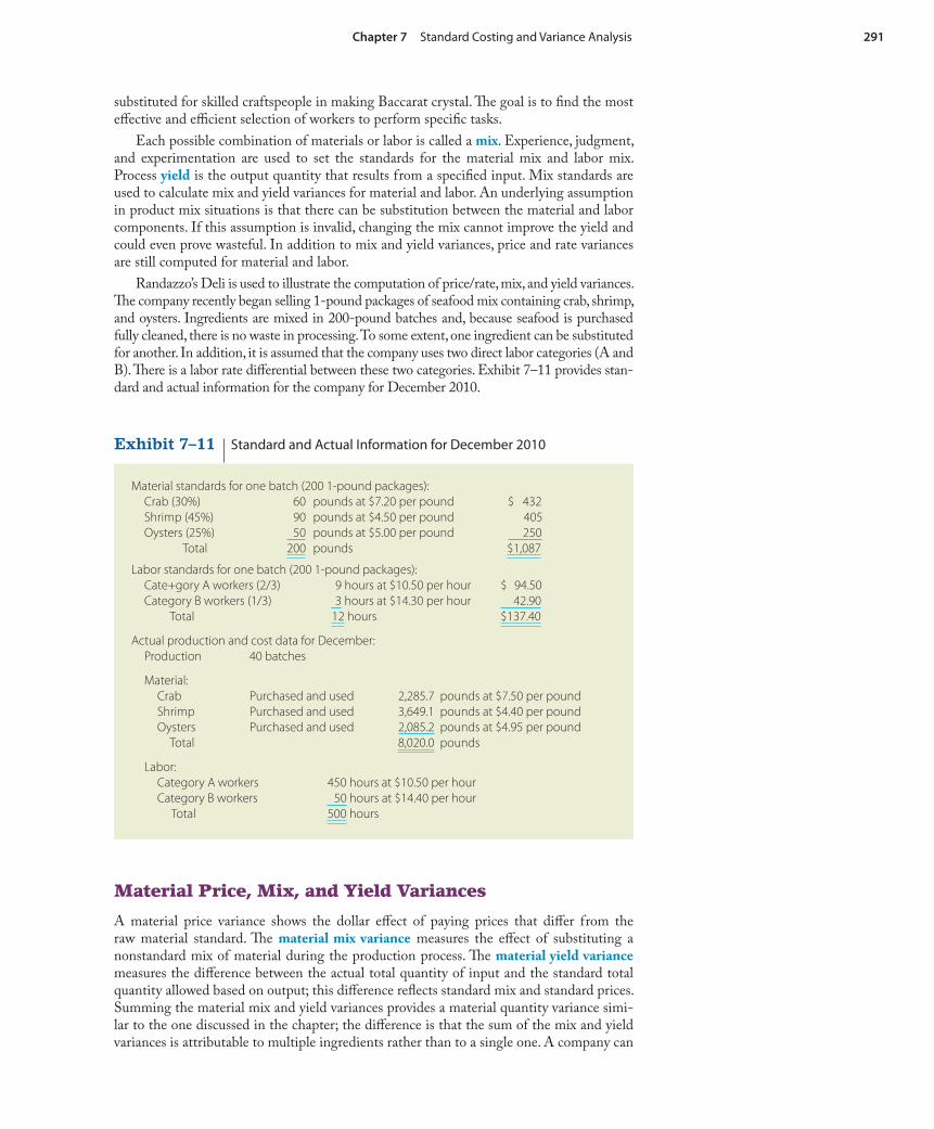
Chapter 7 Standard Costing and Variance Analysis 291
Material Price, Mix, and Yield Variances
A material price variance shows the dollar eff ect of paying prices that diff er from the raw material standard. Th e material mix variance measures the eff ect of substituting a nonstandard mix of material during the production process. Th e material yield variance measures the diff erence between the actual total quantity of input and the standard total quantity allowed based on output; this diff erence refl ects standard mix and standard prices. Summing the material mix and yield variances provides a material quantity variance simi-lar to the one discussed in the chapter; the diff erence is that the sum of the mix and yield variances is attributable to multiple ingredients rather than to a single one. A company can
substituted for skilled craftspeople in making Baccarat crystal. Th e goal is to fi nd the most eff ective and effi cient selection of workers to perform specifi c tasks.
Each possible combination of materials or labor is called a mix. Experience, judgment, and experimentation are used to set the standards for the material mix and labor mix. Process yield is the output quantity that results from a specifi ed input. Mix standards are used to calculate mix and yield variances for material and labor. An underlying assumption in product mix situations is that there can be substitution between the material and labor components. If this assumption is invalid, changing the mix cannot improve the yield and could even prove wasteful. In addition to mix and yield variances, price and rate variances are still computed for material and labor.
Randazzo’s Deli is used to illustrate the computation of price/rate, mix, and yield variances. Th e company recently began selling 1-pound packages of seafood mix containing crab, shrimp, and oysters. Ingredients are mixed in 200-pound batches and, because seafood is purchased fully cleaned, there is no waste in processing. To some extent, one ingredient can be substituted for another. In addition, it is assumed that the company uses two direct labor categories (A and B). Th ere is a labor rate diff erential between these two categories. Exhibit 7–11 provides stan-dard and actual information for the company for December 2010.
Exhibit 7–11 Standard and Actual Information for December 2010
Material standards for one batch (200 1-pound packages):Crab (30%) 60 pounds at $7.20 per pound $ 432Shrimp (45%) 90 pounds at $4.50 per pound 405Oysters (25%) 50 pounds at $5.00 per pound 250
Total 200 pounds $1,087
Labor standards for one batch (200 1-pound packages):Cate+gory A workers (2/3) 9 hours at $10.50 per hour $ 94.50Category B workers (1/3) 3 hours at $14.30 per hour 42.90
Total 12 hours $137.40
Actual production and cost data for December:Production 40 batches
Material:Crab Purchased and used 2,285.7 pounds at $7.50 per poundShrimp Purchased and used 3,649.1 pounds at $4.40 per poundOysters Purchased and used 2,085.2 pounds at $4.95 per pound
Total 8,020.0 pounds
Labor:Category A workers 450 hours at $10.50 per hourCategory B workers 50 hours at $14.40 per hour
Total 500 hours

292 Chapter 7 Standard Costing and Variance Analysis
Given the information in Exhibit 7–11, Randazzo’s Deli used 8,020 total pounds of ingredients to make 40 batches of seafood mix. Th e standard quantity necessary to produce this quantity is 8,000 total pounds of ingredients. Th e actual mix of crab, shrimp, and oys-ters was 28.5, 45.5, and 26.0 percent, respectively:
Crab (2,285.7 pounds of 8,020) � 28.5%
Shrimp (3,649.1 pounds of 8,020) � 45.5%
Oysters (2,085.2 pounds of 8,020) � 26.0%
Computations necessary for the material variances are shown in Exhibit 7–12.
Actual M & Q; Standard P$43,303.99
Actual M, Q, & P*$43,520.53
Standard M; Actual Q; Standard P
$43,588.70
Standard M, Q, & P
$43,480.00$216.54 U
Material Price Variance
$284.71 F
Material Mix Variance
$108.70 U
Material Yield Variance
$40.53 U
* Note: M � mix, Q � quantity, and P � price.
Total Material Variance
Actual Mix � Actual Quantity �
Standard Price
Actual Mix � Actual Quantity �
Actual Price
Standard Mix � Actual Quantity �
Standard Price
Standard Mix � Standard Quantity �
Standard Price
Material Price Variance
Material Mix Variance
Material Yield Variance
Exhibit 7–12 Computations for Material Mix and Yield Variances
(1) Total actual data (mix, quantity, and prices): Crab—2,285.7 pounds � $7.50 $17,142.75 Shrimp—3,649.1 pounds � $4.40 16,056.04 Oysters—2,085.2 pounds � $4.95 10,321.74 $43,520.53(2) Actual mix and quantity; standard prices: Crab—2,285.7 pounds � $7.20 $16,457.04 Shrimp—3,649.1 pounds � $4.50 16,420.95 Oysters—2,085.2 pounds � $5.00 10,426.00 $43,303.99(3) Standard mix; actual quantity; standard prices: Crab—30% � 8,020 pounds � $7.20 $17,323.20 Shrimp—45% � 8,020 pounds � $4.50 16,240.50 Oysters—25% � 8,020 pounds � $5.00 10,025.00 $43,588.70(4) Total standard data (mix, quantity, and prices): Crab—30% � 8,000 pounds � $7.20 $17,280.00 Shrimp—45% � 8,000 pounds � $4.50 16,200.00 Oysters—25% � 8,000 pounds � $5.00 10,000.00 $43,480.00
Th ese computations show a single price variance being calculated for all of the materi-als. To provide more useful information, separate price variances should be calculated for each ingredient. Using the information in Exhibit 7–12, the individual material price vari-ances for crab, shrimp, and oysters are:
Crab � ($17,142.75 � $16,457.04) � $685.71 U
Shrimp � ($16,056.04 � $16,420.95) � �$364.91 F
Oysters � ($10,321.74 � $10,426.00) � �$104.26 F
have a mix variance without experiencing a yield variance. Computations for the price, mix, and yield variances are given in a format similar to that used in the chapter:

Chapter 7 Standard Costing and Variance Analysis 293
Th e savings on shrimp and oysters did not off set the higher price for crab, so the total price variance was unfavorable. Also, less than the standard proportion of the most expensive ingredient (crab) was used, so it is reasonable that there would be a favorable mix vari-ance. Randazzo’s Deli also experienced an unfavorable yield because the 8,020 total actual pounds used was more than the 8,000 total pounds allowed for an output of 40 batches.
Labor Rate, Mix, and Yield Variances
Th e two labor categories used by Randazzo’s Deli are helpers (A) and cooks (B). When labor standards are prepared, the labor categories needed to perform various tasks and the amount of time each task is expected to take are established. During production, variances will occur if workers are not paid the standard rate, do not work in the standard mix on tasks, or do not perform those tasks in the standard time.
Th e labor rate variance is a measure of the cost of paying workers at other than standard rates. Th e labor mix variance is the fi nancial eff ect associated with changing the relative hours of higher- or lower-paid workers in production. Th e labor yield variance refl ects the monetary impact of using a higher- or lower- number of hours than the standard allowed. Th e sum of the labor mix and yield variances equals the labor effi ciency variance. Th e dia-gram for computing labor rate, mix, and yield variances is as follows:
Actual Mix �Actual Hours �Standard Rate
Actual Mix �Actual Hours �
Actual Rate
Standard Mix �Actual Hours �Standard Rate
Standard Mix �Standard Hours �
Standard Rate
Labor Rate Variance Labor Mix Variance Labor Yield Variance
Exhibit 7–13 Computations for Labor Mix and Yield Variances
(1) Total actual data (mix, hours, and rates):
Category A—450 hours � $10.50 $4,725.00
Category B—50 hours � $14.40 720.00 $5,445.00
(2) Actual mix and hours; standard rates:
Category A—450 hours � $10.50 $4,725.00
Category B—50 hours � $14.30 715.00 $5,440.00
(3) Standard mix; actual hours; standard rates:
Category A—75% � 500 � $10.50 $3,937.50
Category B—25% � 500 � $14.40 1,800.00 $5,737.50
(4) Total standard data (mix, hours, and rates):
Category A—75% � 480 � $10.50 $3,780.00
Category B—25% � 480 � $14.30 1,716.00 $5,496.00
Standard rates are used to make both the mix and yield computations. To make the seafood mix, the standard labor time is 12 hours, using 9 hours of category A and 3 hours of category B labor or 75 percent and 25 percent, respectively. Th e actual mix is of labor is:
Category A (450 of 500 hours) � 90%
Category B (50 of 500 hours) � 10%
Exhibit 7–13 provides the labor computations for the seafood mix production. Because 12 hours is the standard for producing one batch of seafood mix, the standard number of hours allowed for production of 40 batches is 480 hours: 360 hours of A and 120 hours of B.
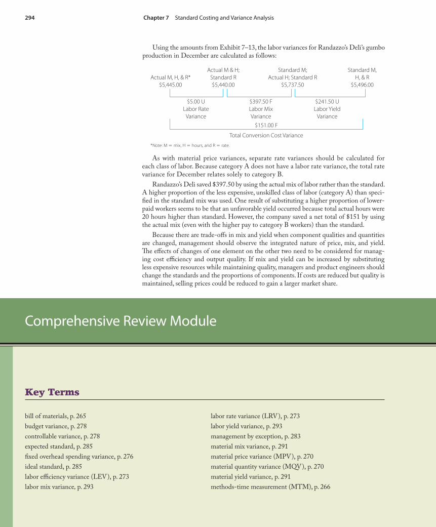
Key Terms
294 Chapter 7 Standard Costing and Variance Analysis
Using the amounts from Exhibit 7–13, the labor variances for Randazzo’s Deli’s gumbo production in December are calculated as follows:
Comprehensive Review Module
As with material price variances, separate rate variances should be calculated for each class of labor. Because category A does not have a labor rate variance, the total rate variance for December relates solely to category B.
Randazzo’s Deli saved $397.50 by using the actual mix of labor rather than the standard. A higher proportion of the less expensive, unskilled class of labor (category A) than speci-fi ed in the standard mix was used. One result of substituting a higher proportion of lower-paid workers seems to be that an unfavorable yield occurred because total actual hours were 20 hours higher than standard. However, the company saved a net total of $151 by using the actual mix (even with the higher pay to category B workers) than the standard.
Because there are trade-off s in mix and yield when component qualities and quantities are changed, management should observe the integrated nature of price, mix, and yield. Th e eff ects of changes of one element on the other two need to be considered for manag-ing cost effi ciency and output quality. If mix and yield can be increased by substituting less expensive resources while maintaining quality, managers and product engineers should change the standards and the proportions of components. If costs are reduced but quality is maintained, selling prices could be reduced to gain a larger market share.
bill of materials, p. 265
budget variance, p. 278
controllable variance, p. 278
expected standard, p. 285
fi xed overhead spending variance, p. 276
ideal standard, p. 285
labor effi ciency variance (LEV), p. 273
labor mix variance, p. 293
labor rate variance (LRV), p. 273
labor yield variance, p. 293
management by exception, p. 283
material mix variance, p. 291
material price variance (MPV), p. 270
material quantity variance (MQV), p. 270
material yield variance, p. 291
methods-time measurement (MTM), p. 266
Actual M & H;Standard R$5,440.00
Actual M, H, & R*$5,445.00
Standard M; Actual H; Standard R
$5,737.50
Standard M,H, & R
$5,496.00
$5.00 ULabor Rate
Variance
$397.50 FLabor MixVariance
$241.50 ULabor Yield
Variance$151.00 F
Total Conversion Cost Variance
* Note: M � mix, H � hours, and R � rate.
Chapter 7 Standard Costing and Variance Analysis 295
mix, p. 291
noncontrollable variance, p. 276
operations fl ow document, p. 267
overhead effi ciency variance, p. 278
overhead spending variance, p. 278
practical standard, p. 285
standard, p. 264
standard cost card, p. 267
standard quantity, p. 269
total cost of ownership (TCO), p. 265
total overhead variance, p. 277
total variance, p. 269
variable overhead effi ciency variance, p. 275
variable overhead spending variance, p. 274
variance analysis, p. 283
volume variance, p. 276
yield, p. 291
LO.1 Setting Material, Labor, and Overhead Standards
Material standards require that management identify the•
types of material inputs needed to make the product -or perform the service.
quality of material inputs needed to make the prod- -uct or perform the service.
quantity of material inputs needed to make the prod- -uct or perform the service.
prices of the material inputs, given normal purchase -quantities.
A bill of materials contains all quantity and quality raw • material specifi cations to make one unit (or batch) of output.
Labor standards require that management identify the•
types of labor tasks needed to make the product or -perform the service.
amount of labor time needed to make the product or -perform the service.
skill levels of personnel needed to make the product -or perform the service.
wage rates or salary levels for the classes of labor -skills needed.
An operations fl ow document contains all labor opera-• tions necessary to make one unit (or batch) of output or perform a particular service.
Overhead standards require that management identify the•
variable and fi xed overhead costs incurred in the -organization.
estimated level of activity to be used in computing -the predetermined overhead rate(s).
estimated variable and fi xed overhead costs at the -estimated level of activity.
predetermined overhead rate(s) used to apply over- -head to production or service performance.
A standard cost card summarizes the standard quanti-• ties and costs needed to complete one unit of product or perform a particular service.
LO.2 Calculating and Recording Material, Labor, and Overhead Variances
Direct material variances are calculated as follows:•
Material Price Variance - � (Actual Price � Actual Quantity) � (Standard Price � Actual Quantity)
Material Quantity Variance - � (Standard Price � Actual Quantity) � (Standard Price � Standard Quantity)
Total Material Variance - � Material Price Variance � Material Quantity Variance
Direct labor variances are calculated as follows:•
Labor Rate Variance - � (Actual Price � Actual Quantity) � (Standard Price � Actual Quantity)
Labor Effi ciency Variance - � (Standard Price � Actual Quantity) � (Standard Price � Standard Quantity)
Total Labor Variance - � Labor Rate Variance � Labor Effi ciency Variance
Variable overhead variances are calculated as follows:•
VOH Spending Variance - � Actual VOH � (Standard Price � Actual Quantity)
VOH Effi ciency Variance - � (Standard Price � Actual Quantity) � Applied VOH
Note: Applied VOH ➢ � (Standard Price � Standard Quantity)
Total VOH Variance - � VOH Spending Variance � VOH Effi ciency Variance
Fixed overhead variances are calculated as follows:•
FOH Spending Variance - � Actual FOH � Budgeted FOH
Note: Budgeted FOH ➢ � Expected FOH amount for the period
Chapter Summary

296 Chapter 7 Standard Costing and Variance Analysis
Volume Variance 5 Budgeted FOH 2 Applied FOH -
Note: Applied FOH ➢ � (Standard Price � Standard Quantity)
Total FOH Variance - � FOH Spending Variance � Volume Variance
A variance is the diff erence between an actual and a • standard cost.
Only standard costs are recorded in the inventory -accounts.
Variances are recorded as either debit (unfavorable) -or credit (favorable) diff erences between the standard cost and the actual cost incurred.
Variances are closed at the end of each accounting -period.
Insignifi cant variances are closed to Cost of ➢Goods Sold.
Signifi cant variances are allocated among Cost of ➢Goods Sold and the appropriate ending inventory accounts.
LO.3 Uses of Standard Costing Systems
A standard cost system is used to•
provide clerical effi ciency. -
assist management in its planning, controlling, deci- -sion making, and performance evaluation functions.
motivate employees when the standards are -
set at a level to encourage high-quality produc- ➢tion and promote cost control.
seen as expected performance goals. ➢
updated periodically so that they refl ect actual ➢economic conditions.
LO.4 Changes in Standard Costing Setting and Usage
In automated companies, the standard cost system may•
use only two elements of production cost: direct -material and conversion.
use ideal standards rather than expected or practical -standards.
use predetermined fi xed overhead rates based on -theoretical capacity rather than expected, normal, or practical capacity.
compute material price variances based on usage -rather than purchases.
LO.5 Standard Costing Using a Conversion Element
If a conversion category is used rather than the tradi-• tional labor and overhead categories,
overhead will commonly be separated into its variable -and fi xed categories.
overhead may be applied using activity-based costing. -
the focus will be on -
spending variances for variable and fi xed ➢overhead.
effi ciency variances for machinery and produc- ➢tion equipment rather than labor.
volume variance for production. ➢
Solution Strategies
Actual Costs (AC), p. 2651. Direct material:
Actual Price (AP) � Actual Quantitiy Purchased or Used (AQ)
DM: AP � AQ � AC
2. Direct labor:
Actual Price (Rate) � Actual Quantity of Hours Worked
DL: AP � AQ � AC
Standard Costs (SC), p. 2681. Direct material:
Standard Price � Standard Quantity
DM: SP � SQ � SC
2. Direct labor:
Standard Price (Rate) � Standard Quantity of Hours
DL: SP � SQ � SC

Chapter 7 Standard Costing and Variance Analysis 297
General Variance Format, p. 269AP � AQ SP � AQ SP � SQ
Material Price VarianceLabor Rate Variance
VOH Spending Variance
Material Quantity VarianceLabor Effi ciency VarianceVOH Effi ciency Variance
Variances in Formula Format, p. 273Th e following abbreviations are used:
AFOH � actual fixed overhead AM � actual mix AP � actual price or rate AQ � actual quantity or hours AVOH � actual variable overhead
BFOH � budgeted fixed overhead (remains at constant amount regardless of activity level as long as within the relevant range)
SM � standard mix SP � standard price SQ � standard quantity TAOH � total actual overhead
Material price variance � (AP � AQ) � (SP � AQ)
Material quantity variance � (SP � AQ) � (SP � SQ)
Labor rate variance � (AP � AQ) � (SP � AQ)
Labor efficiency variance � (SP � AQ) � (SP � SQ)
Four-Variance Approach:
Variable OH spending variance � AVOH � (VOH rate � AQ)Variable OH efficiency variance � (VOH rate � AQ) � (VOH rate � SQ)Fixed OH spending variance � AFOH � BFOHVolume variance � BFOH � (FOH rate � SQ)
Th ree-Variance Approach:
Spending variance � TAOH � [(VOH rate � AQ) � BFOH]Efficiency variance � [(VOH rate � AQ) � BFOH] � [(VOH rate � SQ) � BFOH]Volume variance � [(VOH rate � SQ) � BFOH] � [(VOH rate � SQ) � (FOH rate � SQ)]
(This is equal to the volume variance of the four-variance approach.)
Two-Variance Approach:
Budget variance � TAOH � [(VOH rate � SQ) � BFOH]Volume variance � [(VOH rate � SQ) � BFOH] � [(VOH rate � SQ) � (FOH rate � SQ)]
(This is equal to the volume variance of the four-variance approach.)
One-Variance Approach:
Total OH variance � TAOH � (Combined OH rate � SQ)
(Appendix) Mix and Yield Variances, p. xxMultiple Materials
Material price variance � (AM � AQ � AP) � (AM � AQ � SP)Material mix variance � (AM � AQ � SP) � (SM �AQ � SP)Material yield variance � (SM � AQ � SP) � (SM � SQ � SP)
Multiple Labor Categories
Labor rate variance � (AM � AQ � AP) � (AM � AQ � SP)Labor mix variance � (AM � AQ � SP) � (SM � AQ � SP)Labor yield variance � (SM � AQ � SP) � (SM � SQ � SP)

298 Chapter 7 Standard Costing and Variance Analysis
Variances in Diagram Format, p. 272Direct Material
Point of Purchase
Actual Price � Actual Quantity Purchased
Standard Price � Actual Quantity Purchased
Material Price Variance
Standard Price � Actual Quantity Used
Standard Price � Standard Quantity
Point of Usage
Actual Price � Actual Quantity Used
Standard Price � Actual Quantity Used
Standard Price � Standard Quantity
Direct Labor
Actual Price � Actual Quantity
of Hours Worked
Standard Price � Actual Quantity
of Hours Worked
Standard Price � Standard Quantity
of Hours
Overhead Four-Variance Approach:
Material Quantity Variance
Labor Rate Variance
Material Price Variance Material Quantity Variance
Labor Efficiency Variance
Total Labor Variance
Total Material Variance
Fixed Overhead
Applied VOHVOH Rate � Standard Quantity
VOH Spending Variance VOH Efficiency Variance
Total VOH Variance
(a) (b)VOH Rate � Actual QuantityActual VOH
Variable Overhead
Applied FOHFOH Rate � Standard Quantity
FOH Spending Variance Volume Variance
Total FOH Variance
Budgeted FOHActual FOH
(a) � (c)
(a) � (b) � (c) � (d)
(b) (d)
Overhead One-, Two-, and Th ree-Variance Approaches:
(a) � (b) � (c) (d)
Budget Basedon Input HoursVOH Rate � AQ
� Budgeted FOH
ActualActual VOH
� Actual FOH
Budget Basedon Output
HoursVOH Rate � SQ
� Budgeted FOH
AppliedVOH Rate � SQ
� FOH Rate � SQ
Budget Variance Volume Variance
Spending Variance Efficiency Variance Volume Variance
Total Overhead Variance(Total Underapplied/Overapplied Overhead)

Chapter 7 Standard Costing and Variance Analysis 299
(Appendix) Mix and Yield Variances, p. 290Multiple Materials
Demonstration Problem
Filano Corp. has the following standards for one unit of product:
Direct material: 80 pounds � $6 $480
Direct labor: 3 hours � $16 per hour 48
Variable overhead: 1.5 hours of machine time � $50 per hour 75
Fixed overhead: 1.5 hours of machine time � $30 per hour 45
Th e predetermined OH rates were developed using a practical capacity of 6,000 units per year. Production is assumed to occur evenly throughout the year.
During May 2010, the company produced 525 units. Actual data for May 2010 are as follows:
Direct material purchased: 45,000 pounds � $5.92 per pound
Direct material used: 43,020 pounds (all from May’s purchases)
Total labor cost: $24,955 for 1,550 hours
Variable overhead incurred: $43,750 for 800 hours of machine time
Fixed overhead incurred: $22,800 for 800 hours of machine time
Required:a. Calculate the following:
1. Material price variance based on purchases
2. Material quantity variance
3. Labor rate variance
4. Labor effi ciency variance
5. Variable overhead spending and effi ciency variances
6. Fixed overhead spending and volume variances
7. Overhead variances using a three-variance approach
8. Overhead variances using a two-variance approach
9. Overhead variance using a one-variance approach
b. Record the entries to recognize the variances.
Actual Mix � Actual Quantity �
Standard Price
Actual Mix � Actual Quantity �
Actual Price
Standard Mix � Actual Quantity �
Standard Price
Standard Mix � Standard Quantity �
Standard Price
Material Price Variance Material Mix Variance Material Yield Variance
Actual Mix � Actual Hours � Standard Rate
Actual Mix � Actual Hours �
Actual Rate
Standard Mix � Actual Hours � Standard Rate
Standard Mix � Standard Hours �
Standard Rate
Labor Rate Variance Labor Mix Variance Labor Yield Variance
Multiple Labor Categories

300 Chapter 7 Standard Costing and Variance Analysis
SP � AQp
$6.00 � 45,000$270,000
AP � AQp
$5.92 � 45,000$266,400
$3,600 FMPV
SP � SQ$6 � 42,000
$252,000
SP � AQu
$6 � 43,020$258,120
$6,120 U
MQV
SP � AQ$16 � 1,550
$24,800
AP � AQ$16.10 � 1,550
$24,955
SP � SQ$16 � 1,575
$25,200$155 U
LRV$400 F
LEV
SP � AQ$50.00 � 800
$40,000Actual VOH
$43,750
SP � SQ$50.00 � 787.5
$39,375$3,750 U
VOH Spending Variance$625 U
VOH Effi ciency Variance
Budgeted FOH$22,500
Actual FOH$22,800
SP � SQ $30 � 787.50
$23,625$300 U
FOH Spending Variance$1,125 F
Volume Variance
VOH Rate � SQ � Budgeted FOH
$50 � 787.5 � $39,375
�22,500 $61,875
Actual OH$66,550
Applied OH(SP � SQ)
$80 � 787.50 � $63,000$4,675 U
Budget Variance$1,125 F
Volume Variance
Solution to Demonstration Problema. 1.
2. SQ � 525 � 80 pounds � 42,000 pounds
3. & 4. AR � $24,955 � 1,550 hours � $16.10 per hour
SQ � 525 � 3 hours � 1,575 hours
5. SQ � 525 � 1.5 � 787.5 hours
6. BFOH, annually � 6,000 � 1.5 hours � $30 � $270,000 BFOH, monthly � $270,000 � 12 months � $22,500
SQ � 787.5 hours [from part (5)]
VOH Rate � SQ � Budgeted FOH
$50 � 787.5 � $ 39,375 �22,500 $ 61.875
Applied OH (SP � SQ)
$50 � 787.5 � $39,375� 30 � 787.5 � 23,625 $80 � 787.5 � $63,000
VOH Rate � AQ � Budgeted FOH
$50 � 800 � $ 40,000 �22,500 $62,500
Actual VOH � Actual FOH
$43,750 �22,800 $66,550
$4,050 U Spending Variance
$625 UEffi ciency Variance
$1,125 FVolume Variance
7.–9. Combined overhead application rate � $50 � $30 � $80 per MH; SQ � 787.5 hours [from part (5)].

Chapter 7 Standard Costing and Variance Analysis 301
b. All amounts are taken from the computations shown in part (a).
Raw Material Inventory 270,000
Material Purchase Price Variance 3,600
Accounts Payable 266,400
To record acquisition of material
Work in Process Inventory 252,000
Material Quantity Variance 6,120
Raw Material Inventory 258,120
To record issuance of material to production
Work in Process Inventory 25,200
Labor Rate Variance 155
Wages Payable 24,955
Labor Effi ciency Variance 400
To record direct labor costs in all departments
Work in Process Inventory 39,375
Variable Overhead Effi ciency Variance 3,750
Variable Overhead Spending Variance 625
Variable Manufacturing Overhead Control 43,750
To close variable OH
Work in Process Inventory 23,625
Fixed Overhead Spending Variance 300
Fixed Manufacturing Overhead Control 22,800
Volume Variance 1,125
To close fi xed OH
Ethics
Applied OH SP � SQ
$80 � 787.50 � $63,000Actual OH
$66,550$3,550 U
Total Overhead Variance(Total Underapplied Overhead)
Potential Ethical Issues
1. Setting labor time standards extremely high so that variances on which performance is evaluated are consistently favorable
2. Evaluating each manager on the variances generated in his or her production area without regard for potential implications on other production areas
3. Estimating production at levels signifi cantly higher than is necessary to meet current and anticipated sales, thereby lowering the predetermined fi xed OH rate per unit and inventory cost, while increasing reported operating income
4. Producing unnecessary inventory to generate a high, favorable volume variance

302 Chapter 7 Standard Costing and Variance Analysis
5. Not adjusting standards for changed production conditions so that favorable variances will result
6. Using inappropriate material or labor mixes that create favorable price or rate variances but result in a lower-quality product
Questions
1. What is a standard cost card? What information does it contain? How does it relate to a bill of materials and an operations fl ow document?
2. How is the material standard developed? Why are the quantities shown in the bill of materials not always the same quantities shown in the standard cost card?
3. A total variance can be calculated for each cost component of a product. Into what variances can this total be separated and to what does each relate? (Discuss separately for material and labor.)
4. What is meant by the term standard hours? Does the term refer to inputs or outputs?
5. Th e overhead spending and overhead effi ciency variances are said to be controllable, but the volume variance is said to be noncontrollable. Explain.
6. How are actual and standard costs recorded in a standard cost system?
7. How are insignifi cant variances closed at the end of an accounting period? How are signifi cant variances closed at the end of an accounting period? Why is there a diff er-ence in treatment?
8. What are the three primary uses of a standard cost system? In a business that routinely manufactures the same products or performs the same services, why are standards helpful?
9. What is management by exception? Why is a standard cost system useful when man-agers control “by exception”?
10. Why do managers care about capacity utilization? Are managers controlling costs when they control utilization?
11. (Appendix) What variances can be computed for direct material and direct labor when some materials or labor inputs are substitutes for others? What information does each of these variances provide?
Exercises
12. LO.1 (Standard setting; team project) As a three-person team, choose an activity that is commonly performed every day, such as taking a shower/bath, preparing a meal, or doing homework. Have each team member time him- or herself performing that activity for two days and then develop a standard time for the team. Now have the team members time themselves performing the same activity for the next fi ve days.
a. Using an assumed hourly wage rate of $12, calculate the labor effi ciency variance for your team.
b. Prepare a list of reasons for the variance.
c. How could some of the variance have been avoided?
13. LO.1 (Developing standard cost card; discussion) One of Sure-Bet Sherbet’s best- selling products is raspberry sherbet, which is manufactured in 10-gallon batches. Each
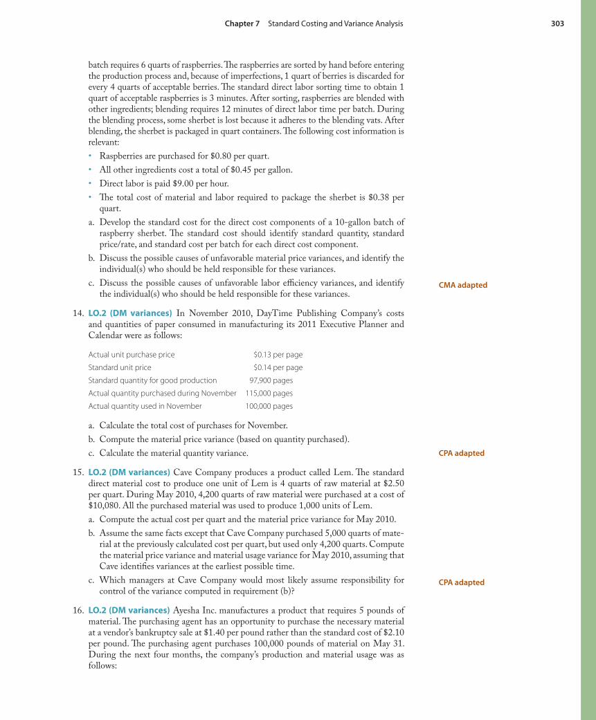
CPA adapted
CPA adapted
Chapter 7 Standard Costing and Variance Analysis 303
batch requires 6 quarts of raspberries. Th e raspberries are sorted by hand before entering the production process and, because of imperfections, 1 quart of berries is discarded for every 4 quarts of acceptable berries. Th e standard direct labor sorting time to obtain 1 quart of acceptable raspberries is 3 minutes. After sorting, raspberries are blended with other ingredients; blending requires 12 minutes of direct labor time per batch. During the blending process, some sherbet is lost because it adheres to the blending vats. After blending, the sherbet is packaged in quart containers. Th e following cost information is relevant:
Raspberries are purchased for $0.80 per quart.•
All other ingredients cost a total of $0.45 per gallon.•
Direct labor is paid $9.00 per hour.•
Th e total cost of material and labor required to package the sherbet is $0.38 per • quart.
a. Develop the standard cost for the direct cost components of a 10-gallon batch of raspberry sherbet. Th e standard cost should identify standard quantity, standard price/rate, and standard cost per batch for each direct cost component.
b. Discuss the possible causes of unfavorable material price variances, and identify the individual(s) who should be held responsible for these variances.
c. Discuss the possible causes of unfavorable labor effi ciency variances, and identify the individual(s) who should be held responsible for these variances.
14. LO.2 (DM variances) In November 2010, DayTime Publishing Company’s costs and quantities of paper consumed in manufacturing its 2011 Executive Planner and Calendar were as follows:
Actual unit purchase price $0.13 per page
Standard unit price $0.14 per page
Standard quantity for good production 97,900 pages
Actual quantity purchased during November 115,000 pages
Actual quantity used in November 100,000 pages
a. Calculate the total cost of purchases for November.
b. Compute the material price variance (based on quantity purchased).
c. Calculate the material quantity variance.
15. LO.2 (DM variances) Cave Company produces a product called Lem. Th e standard direct material cost to produce one unit of Lem is 4 quarts of raw material at $2.50 per quart. During May 2010, 4,200 quarts of raw material were purchased at a cost of $10,080. All the purchased material was used to produce 1,000 units of Lem.
a. Compute the actual cost per quart and the material price variance for May 2010.
b. Assume the same facts except that Cave Company purchased 5,000 quarts of mate-rial at the previously calculated cost per quart, but used only 4,200 quarts. Compute the material price variance and material usage variance for May 2010, assuming that Cave identifi es variances at the earliest possible time.
c. Which managers at Cave Company would most likely assume responsibility for control of the variance computed in requirement (b)?
16. LO.2 (DM variances) Ayesha Inc. manufactures a product that requires 5 pounds of material. Th e purchasing agent has an opportunity to purchase the necessary material at a vendor’s bankruptcy sale at $1.40 per pound rather than the standard cost of $2.10 per pound. Th e purchasing agent purchases 100,000 pounds of material on May 31. During the next four months, the company’s production and material usage was as follows:

Production Quantity Used
June 3,000 16,400 lb.
July 3,400 17,540 lb.
August 2,900 14,950 lb.
September 2,500 13,200 lb.
a. What is the material price variance for this purchase?
b. What is the material quantity variance for each month for this material?
c. What might be the cause of the unfavorable material quantity variances?
17. LO.2 (DM variances) A&G makes wrought iron table and chair sets. During April, the purchasing agent bought 25,600 pounds of scrap iron at $1.94 per pound. During the month, 21,400 pounds of scrap iron were used to produce 600 table and chair sets. Each set requires a standard quantity of 35 pounds at a standard cost of $1.90 per pound.
a. For April, compute the direct material price variance (based on the quantity pur-chased) and the direct material quantity variance (based on quantity used).
b. Identify the titles of individuals in the fi rm who would be responsible for each of the variances.
c. Provide some possible explanations for the variances computed in part (a).
18. LO.2 (DL variances) Heath Construction builds standard prefabricated wooden frames for walls. Each frame requires 10 direct labor hours and the standard hourly direct labor rate is $18. During July, the company produced 670 frames and worked 6,800 direct labor hours. Payroll records indicate that workers earned $127,500.
a. What were the standard hours for July construction?
b. Calculate the direct labor variances.
c. What was the actual hourly wage rate?
19. LO.2 (DL variances) Information on Hanley’s direct labor costs for January 2010 is as follows:
Actual direct labor rate $7.50
Standard direct labor hours allowed 11,000
Actual direct labor hours 10,000
Direct labor rate variance $5,500 F
a. Compute the standard direct labor rate in January.
b. Compute the labor effi ciency variance in January.
c. Prepare the journal entry to accrue direct labor cost and to record the labor variances for January.
d. Prepare the journal entry to dispose of the January labor variances, assuming that they are insignifi cant.
20. LO.2 (DL variances) Calista & Lane, CPAs, set the following standard for its inven-tory audit of Triumph Co.: 350 hours at an average hourly billing rate of $250. Th e fi rm actually worked 330 hours during the inventory audit process. Th e total labor variance for the audit was $3,500 unfavorable.
a. Compute the total actual payroll.
b. Compute the labor effi ciency variance.
c. Compute the labor rate variance.
304 Chapter 7 Standard Costing and Variance Analysis
CPA adapted

Chapter 7 Standard Costing and Variance Analysis 305
d. Prepare the entry to assign labor costs to inventory, record the labor variances, and accrue payroll costs.
e. Write a memo to the appropriate personnel regarding feedback about the labor effi ciency variance. Th e memo should also off er a brief explanation that is consistent with the labor rate and effi ciency variances.
21. LO.2 (Missing information for DL) For each independent case, fi ll in the missing fi gures.
Case A Case B Case C Case D
Units produced 1,000 ? 240 1,500
Standard hours per unit 3.5 0.9 ? ?
Standard hours ? 900 600 ?
Standard rate per hour $ 7.25 ? $ 10.50 $ 7
Actual hours worked 3,400 975 ? 4,900
Actual labor cost ? ? $ 6,180 $ 31,850
Labor rate variance $850 F $975 F $300 U ?
Labor effi ciency variance ? $765 U ? $2,800 U
22. LO.2 (DM & DL variances) In July 2010, Zinger Corp. purchased 20,000 gallons of Numerol for $61,000 to use in the production of product #43MR7. During July, Zinger Corp. manufactured 3,900 units of product #43MR7. Th e following informa-tion is available about standard and actual quantities and costs:
Standard for One Unit Actual Usage for July
Direct material 4.8 gallons @ $3 per gallon 18,350 gallons
Direct labor 20 minutes @ $9 per DLH 1,290 DLHs @ $9.02 per DLH
a. Compute the material purchase price variance and the material quantity variance.
b. Compute the labor rate, labor effi ciency, and total labor variance.
23. LO.2 (DM & DL variances) Madzinga’s Draperies manufactures curtains. Curtain #4571 requires the following:
Direct material standard 10 square yards at $5 per yard
Direct labor standard 5 hours at $10 per hour
During the second quarter, the company purchased 17,000 square yards at a cost of $83,300 and used 16,500 square yards to produce 1,500 Curtain #4571s. Direct labor totaled 7,600 hours for $79,800.
a. Compute the material price and usage variances.
b. Prepare the journal entries for the purchase and use of direct material.
c. Compute labor rate and labor effi ciency variances.
d. Prepare the journal entry to accrue direct labor cost and record the labor variances for the quarter.
e. Comment on the above variances. Identify possible causes and relationships among the variances that you computed.
24. LO.2 (DM & DL variances) Green Tee produces 100 percent cotton t-shirts, with the following standard direct material and labor quantities and costs:
Direct material 2.0 yards � $3.00
Direct labor 0.7 hour � $7.50

306 Chapter 7 Standard Costing and Variance Analysis
Actual September production and costs for the company to produce 10,000 t-shirts were as follows:
Quantity Cost
Direct material
Purchased 30,000 yards $89,700
Requisitioned into production 20,120 yards
Direct labor 7,940 hours 58,756
a. What is the standard quantity of material and the standard labor time for September’s production?
b. Compute the direct material and direct labor variances.
c. How might the sales and production managers explain the direct material variances?
d. How might the production and human resources managers explain the direct labor variances?
e. Record the year-end adjusting entry to close the material and labor variances.
25. LO.2 (DM & DL variances) In December, Sam Antari, president of Antari Inc., received the following information from Denise Sweet, the new controller, in regard to November production of travel bags:
November production 4,800 bags
Actual cost of material purchased and used $14,550
Standard material allowed 0.5 square yard per bag
Material quantity variance $600 U
Standard price per yard of material $ 6
Actual hours worked 9,760 hours
Standard labor time per bag 2 hours
Labor rate variance $1,464 F
Standard labor rate per hour $17
Antari asked Sweet to provide the following information:
a. Standard quantity of material allowed for November production
b. Standard direct labor hours allowed for November production
c. Material price variance
d. Labor effi ciency variance
e. Standard prime (direct material and direct labor) cost to produce one travel bag
f. Actual cost to produce one travel bag in November
g. An explanation for the diff erence between standard and actual cost; be sure that the explanation is consistent with the pattern of the variances
26. LO.2 (OH variances) Edina Co. manufactures a product that requires 3.5 machine hours per unit. Th e variable and fi xed overhead rates were computed using expected capacity of 144,000 units (produced evenly throughout the year) and expected vari-able and fi xed overhead costs, respectively, of $2,016,000 and $3,528,000. In October, Edina manufactured 11,800 units using 40,800 machine hours. October variable over-head costs were $171,000; fi xed overhead costs were $284,500.
a. What are the standard variable and fi xed overhead rates?
b. Compute the variable overhead variances.
c. Compute the fi xed overhead variances.
d. Explain the volume variance computed in part (c).
Excel

Chapter 7 Standard Costing and Variance Analysis 307
27. LO.2 (OH variances) FUN Inc. has a fully automated production facility in which almost 97 percent of overhead costs are driven by machine hours. As the company’s cost accountant, you have computed the following overhead variances for May:
Variable overhead spending variance $34,000 F
Variable overhead effi ciency variance 41,200 F
Fixed overhead spending variance 28,000 U
Fixed overhead volume variance 20,000 U
Th e company’s president is concerned about the variance amounts and has asked you to show her how the variances were computed and to answer several questions. Bud-geted fi xed overhead for the month is $1,000,000; the predetermined variable and fi xed overhead rates are, respectively, $20 and $40 per machine hour. Budgeted capacity is 20,000 units.
a. Using the four-variance approach, prepare an overhead analysis in as much detail as possible.
b. What is the standard number of machine hours allowed for each unit of output?
c. How many actual hours were worked in May?
d. What is the total spending variance?
e. What additional information about the manufacturing overhead variances is gained by inserting detailed computations into the variable and fi xed manufacturing over-head variance analysis?
f. How would the overhead variances be closed if the three-variance approach were used?
28. LO.2 (OH variances) Th e manager of the Texas Department of Transportation has determined that it typically takes 30 minutes for the department’s employees to regis-ter a new car. In Bexar County, the predetermined fi xed overhead rate was computed on an estimated 10,000 direct labor hours per month and is $9 per direct labor hour, whereas the predetermined variable overhead rate is $3 per direct labor hour.
During July, 18,800 cars were registered in Bexar County and 9,500 direct labor hours were worked in registering those vehicles. For the month, variable overhead was $27,700 and fi xed overhead was $90,800.
a. Compute overhead variances using a four-variance approach.
b. Compute overhead variances using a three-variance approach.
c. Compute overhead variances using a two-variance approach.
29. LO.2 (Four OH variances; journal entries) Kemp Manufacturing set 70,000 direct labor hours as the 2010 capacity measure for computing its predetermined variable overhead rate. At that level, budgeted variable overhead costs are $315,000. Kemp will apply budgeted fi xed overhead of $140,400 on the basis of 3,900 budgeted machine hours for the year. Both machine hours and fi xed overhead costs are expected to be incurred evenly each month.
During March 2010, Kemp incurred 5,900 direct labor hours and 300 machine hours. Actual variable and fi xed overhead were $26,325 and $11,400, respectively. Th e standard times allowed for March production were 5,980 direct labor hours and 290 machine hours.
a. Using the four-variance approach, determine the overhead variances for March 2010.
b. Prepare all journal entries related to overhead for Kemp Manufacturing for March 2010.
30. LO.2 (Three OH variances) Munich Ltd. uses a combined overhead rate of $2.90 per machine hour to apply overhead to products. Th e rate was developed at an expected
Excel
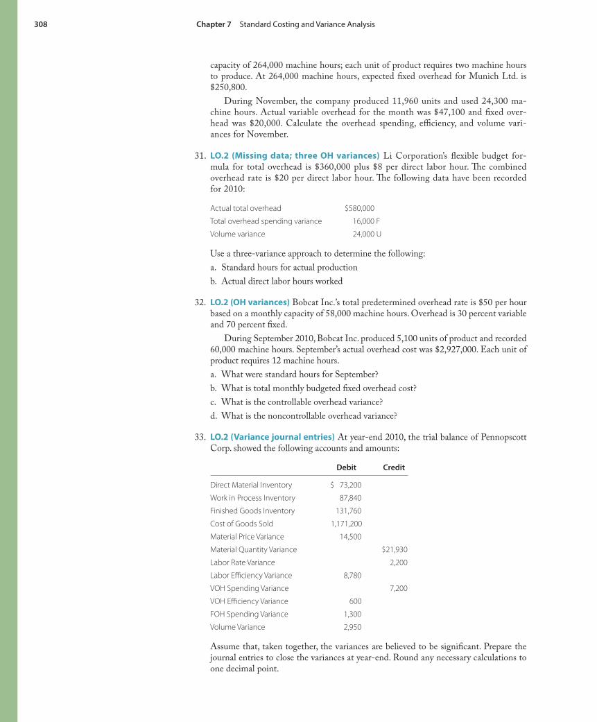
308 Chapter 7 Standard Costing and Variance Analysis
capacity of 264,000 machine hours; each unit of product requires two machine hours to produce. At 264,000 machine hours, expected fi xed overhead for Munich Ltd. is $250,800.
During November, the company produced 11,960 units and used 24,300 ma-chine hours. Actual variable overhead for the month was $47,100 and fi xed over-head was $20,000. Calculate the overhead spending, effi ciency, and volume vari-ances for November.
31. LO.2 (Missing data; three OH variances) Li Corporation’s fl exible budget for-mula for total overhead is $360,000 plus $8 per direct labor hour. Th e combined overhead rate is $20 per direct labor hour. Th e following data have been recorded for 2010:
Actual total overhead $580,000
Total overhead spending variance 16,000 F
Volume variance 24,000 U
Use a three-variance approach to determine the following:
a. Standard hours for actual production
b. Actual direct labor hours worked
32. LO.2 (OH variances) Bobcat Inc.’s total predetermined overhead rate is $50 per hour based on a monthly capacity of 58,000 machine hours. Overhead is 30 percent variable and 70 percent fi xed.
During September 2010, Bobcat Inc. produced 5,100 units of product and recorded 60,000 machine hours. September’s actual overhead cost was $2,927,000. Each unit of product requires 12 machine hours.
a. What were standard hours for September?
b. What is total monthly budgeted fi xed overhead cost?
c. What is the controllable overhead variance?
d. What is the noncontrollable overhead variance?
33. LO.2 (Variance journal entries) At year-end 2010, the trial balance of Pennopscott Corp. showed the following accounts and amounts:
Debit Credit
Direct Material Inventory $ 73,200
Work in Process Inventory 87,840
Finished Goods Inventory 131,760
Cost of Goods Sold 1,171,200
Material Price Variance 14,500
Material Quantity Variance $21,930
Labor Rate Variance 2,200
Labor Effi ciency Variance 8,780
VOH Spending Variance 7,200
VOH Effi ciency Variance 600
FOH Spending Variance 1,300
Volume Variance 2,950
Assume that, taken together, the variances are believed to be signifi cant. Prepare the journal entries to close the variances at year-end. Round any necessary calculations to one decimal point.
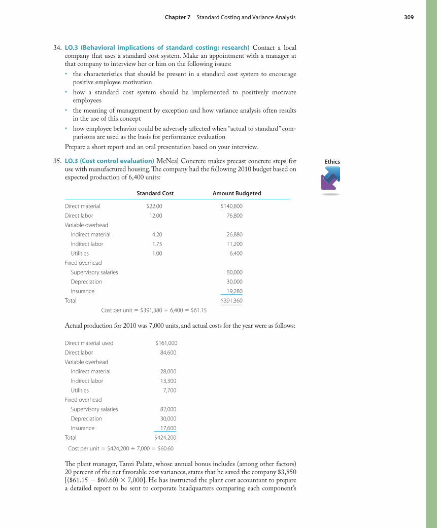
Chapter 7 Standard Costing and Variance Analysis 309
34. LO.3 (Behavioral implications of standard costing; research) Contact a local company that uses a standard cost system. Make an appointment with a manager at that company to interview her or him on the following issues:
the characteristics that should be present in a standard cost system to encourage • positive employee motivation
how a standard cost system should be implemented to positively motivate • employees
the meaning of management by exception and how variance analysis often results • in the use of this concept
how employee behavior could be adversely aff ected when “actual to standard” com-• parisons are used as the basis for performance evaluation
Prepare a short report and an oral presentation based on your interview.
35. LO.3 (Cost control evaluation) McNeal Concrete makes precast concrete steps for use with manufactured housing. Th e company had the following 2010 budget based on expected production of 6,400 units:
Standard Cost Amount Budgeted
Direct material $22.00 $140,800
Direct labor 12.00 76,800
Variable overhead
Indirect material 4.20 26,880
Indirect labor 1.75 11,200
Utilities 1.00 6,400
Fixed overhead
Supervisory salaries 80,000
Depreciation 30,000
Insurance 19,280
Total $391,360
Cost per unit � $391,380 � 6,400 � $61.15
Actual production for 2010 was 7,000 units, and actual costs for the year were as follows:
Direct material used $161,000
Direct labor 84,600
Variable overhead
Indirect material 28,000
Indirect labor 13,300
Utilities 7,700
Fixed overhead
Supervisory salaries 82,000
Depreciation 30,000
Insurance 17,600
Total $424,200
Cost per unit � $424,200 � 7,000 � $60.60
Th e plant manager, Tanzi Palate, whose annual bonus includes (among other factors) 20 percent of the net favorable cost variances, states that he saved the company $3,850 [($61.15 � $60.60) � 7,000]. He has instructed the plant cost accountant to prepare a detailed report to be sent to corporate headquarters comparing each component’s
Ethics

310 Chapter 7 Standard Costing and Variance Analysis
actual per-unit cost with the per-unit amounts in the preceding annual budget to prove the $3,850 cost savings.
a. Is the actual-to-budget comparison proposed by Palate appropriate? If his compari-son is not appropriate, prepare a more appropriate comparison.
b. How would you, as the plant cost accountant, react if Palate insisted on his compari-son? Suggest what alternatives are available to you.
36. LO.3 (Ethics; writing) Hotel rooms have become more extravagant over the past decade and the time needed to clean a room has increased. According to a study enti-tled “Creating Luxury, Enduring Pain” by Unite Here (the primary union representing hotel workers in the United States), housekeepers have the most dangerous jobs at hotels and have an injury rate of more than one in ten workers—almost twice that of other hotel employees. In 2001, the standard number of rooms for a housekeeper to clean had risen from 12 per day to 18 per day. At one pricey hotel chain, it was esti-mated that a housekeeper who cleaned 15 rooms stripped approximately 500 pounds of soiled linens and replaced those with 500 pounds of clean linens . . . resulting in back and shoulder injuries, carpal tunnel syndrome, and bursitis.
Two articles relating to this situation are Komp, “How Hotel Work Is Hurt-ing Housekeepers,” Ergoweb (May 10, 2006) (http://www.ergoweb.com/news/detail.cfm?print=on&id=1616; last accessed 4/26/09) and Frumin et al., “Workload-Related Musculoskeletal Disorders among Hotel Housekeepers: Employer Records Reveal a Growing National Problem” (April 19, 2006) (http://www.hotelworkersrising.org/pdf/hskpr_analysis0406.pdf; last accessed 4/26/09).
a. Why is it necessary for hotels to establish a standard for number of rooms to be cleaned by housekeepers?
b. Th e average annual wages of housekeepers is $17,340, although this may be higher at the larger hotel chains. Th e large hotel chains are, however, attempting to elimi-nate health-care benefi ts with the wage increases. Given the rate of job injuries, do you believe that the housekeepers are better off with the lower wage and health-care benefi ts or a higher wage and no health-care benefi ts? Explain.
c. In an 8-hour day (480 minutes), cleaning 15 rooms amounts to approximately 32 minutes per room. What makes it diffi cult for a housekeeper to strip and remake a bed, vacuum, lightly dust, and clean a bathroom in that period of time?
37. LO.3 (DL & OH; use of standard cost systems; ethics; writing) Many companies face the prospect of paying workers overtime wages; some of these payments are at time-and-a-half wages.
a. How does overtime pay aff ect direct labor cost? Variable overhead?
b. Obviously, paying overtime to already employed workers makes better fi nancial business sense than does hiring additional workers. If workers would prefer not to work overtime but do so to maintain their jobs, how does overtime aff ect the ethical contract between employers and employees?
c. What eff ects might overtime have on job effi ciency? On job eff ectiveness (such as quality of production)?
d. Would you be in favor of limiting allowable hours of overtime to have more indi-viduals employed? Discuss this question from the standpoint of (1) the govern-ment, (2) the employer, (3) a currently employed worker, and (4) an unemployed individual.
38. LO.3 (Ethics; writing) An HMO medical program began reimbursing hospitals according to diagnostic-related groups (DRGs). Each DRG has a specifi ed stan-dard “length of stay.” If a patient leaves the hospital early, the hospital is fi nancially
Ethics
Internet
Ethics
Ethics

Chapter 7 Standard Costing and Variance Analysis 311
impacted favorably, but a patient staying longer than the specifi ed time costs the hos-pital money.
a. From the hospital administrator’s point of view, would you want favorable length-of-stay variances? How might you try to obtain such variances?
b. From a patient’s point of view, would you want favorable length-of-stay variances? Answer this question from the point of view of (1) a patient who has had minor surgery and (2) a patient who has had major surgery.
c. Would favorable length-of-stay variances necessarily equate to high-quality care?
39. LO.5 (Variances and conversion cost category) Auto Brakes Inc. manufactures brake rotors and has always applied overhead to production using direct labor hours. Recently, company facilities were automated, and the accounting system was revised to show only two cost categories: direct material and conversion. Estimated variable and fi xed conver-sion costs for the current month were $170,000 and $76,000, respectively. Expected output for the current month was 5,000 rotors and the estimated number of machine hours was 10,000. During July 2010, the fi rm actually used 9,000 machine hours to make 4,800 rotors while incurring $228,000 of conversion costs. Of this amount, $150,000 was variable cost.
a. Using the four-variance approach, compute the variances for conversion costs.
b. Evaluate the eff ectiveness of the fi rm in controlling the current month’s costs.
40. LO.5 (Variances and conversion cost category) Svenson Technology considers direct labor cost too insignifi cant to separately account for, and, therefore, uses a $22.50 per machine hour predetermined conversion cost rate (of which $16 is related to fi xed over-head costs). Th e conversion rate was established based on expected capacity of 1,008,600 machine hours. One of Svenson Technology’s products requires 4.1 machine hours to manufacture.
In September 2010, the company manufactured 21,000 units of product and used 83,000 machine hours and 840 direct labor hours. Variable and fi xed conversion costs incurred for September were $551,230 and $1,330,000, respectively.
a. What is the expected capacity per month in units and machine hours?
b. Prepare a four- and three-variance analysis of conversion costs for September 2010.
41. LO.6 (Appendix) Hennessey Company produces 12-ounce cans of mixed pecans and cashews. Standard and actual information follows.
Standard Quantities and Costs (12-oz. can)
Pecans: 6 ounces at $6.00 per pound $2.25
Cashews: 6 ounces at $8.00 per pound 3.00
Actual Quantities and Costs for Production of 36,000 Cans
Pecans: 15,554 pounds at $5.80 per pound
Cashews: 12,726 pounds at $8.50 per pound
Determine the material price, mix, and yield variances.
42. LO.6 (Appendix) Coff en Corp. employs engineers and draftspeople. Th e average hourly rates are $60 for engineers and $30 for draftspeople. For one project, the stan-dard was set at 400 hours of engineer time and 600 hours of draftsperson time. Actual hours worked on this project were:
Engineers—500 hours at $65 per hour
Draftspeople—500 hours at $32 per hour
Determine the labor rate, mix, and yield variances for this project.
312 Chapter 7 Standard Costing and Variance Analysis
43. LO.6 (Appendix) Bernie Services has three labor classes: administrative assistants, para-legals, and attorneys. Standard wage rates are as follows: administrative assistants, $30 per hour; paralegals, $60 per hour; and attorneys, $125 per hour. For October, the num-bers of actual direct labor hours worked and of standard hours for probate cases were as follows:
Actual DLHs Number of Standard Hours Allowed
Administrative assistant 900 1,008
Paralegal 2,520 2,772
Attorney 1,500 1,260
a. Calculate October’s direct labor effi ciency variance and decompose the total into the following components:
1. direct labor mix variance, and
2. direct labor yield variance.
b. Prepare a memo addressing whether management used an effi cient mix of labor.
Problems
44. LO.2 (DM & DL variances) Schmidt Co. has the following standard material and labor quantities and costs for one unit of Product SWK#468:
Material 1.85 pounds @ $3.50 per pound
Labor 0.04 hours @ $12 per hour
During July, the purchasing agent found a “good deal” on the raw material needed for Product SWK#468 and bought 100,000 pounds of material at $3.15 per pound. In July, the company produced 48,000 units of Product SWK#468 with the following material and labor usage:
Material 95,000 pounds
Labor 2,200 hours @ $12.10 (due to a renegotiated labor contract)
a. What is the standard quantity of material and the standard labor time for July?
b. Calculate the material and labor variances for July.
c. Did the purchasing agent make a “good deal” on the raw material? Explain.
45. LO.2 (DM & DL variances; journal entries) Griff on Corp. makes small plastic dog toys with the following material and labor standards:
Standard Quantity Standard Cost
Material 0.5 pound $4.00 per pound
Labor 12 minutes 9.00 per hour
During October, 60,000 pounds of material were acquired on account at $4.15 per pound. During October, 50,120 pounds of that were used in production during the month to make 100,000 toys. Factory payroll for October showed 20,600 direct labor hours at a total cost of $182,310.
a. Compute material and labor variances, basing the material price variance on the quantity of material purchased.
b. Assuming a perpetual inventory system is used, prepare the relevant general journal entries for October.
Chapter 7 Standard Costing and Variance Analysis 313
46. LO.2 (DM & DL variances) Aquatica uses a standard cost system for materials and labor in producing small fi shing boats. Production requires three materials: fi berglass, paint, and a purchased trim package. Th e standard costs and quantities for materials and labor are as follows:
Standards for One Fishing Boat
2,000 pounds of fi berglass � $1.80 per pound $3,600
6 quarts gel coat paint � $15.00 per quart 90
1 trim package 200
40 hours of labor � $25.00 per hour 1,000
Standard cost for DM and DL $4,890
Th e following actual data related to the production of 600 boats was recorded for July:
Material Purchased on Account
Fiberglass—2,100,000 pounds � $1.83 per pound
Paint—1,000 gallons � $55.50 per gallon
Trim packages—640 � $205 per package
Material Used
Fiberglass—1,380,000 pounds
Paint—924 gallons
Trim packages—608
Direct Labor Used
23,850 hours � $23.50 per hour
Calculate the material and labor variances for Aquatica for July. Th e material price vari-ance should be computed for each type of material and on the quantity of material purchased.
47. LO.2 (Incomplete data; variances) Surgical Products produces latex surgical gloves. Machines perform the majority of the processing for 1,000 pairs of gloves per hour. Each pair of gloves requires 0.85 square foot of latex, which has a standard price of $0.80 per square foot. Machine operators are considered direct labor and are paid $15 per hour.
During one week in May, Surgical Products produced 300,000 pairs of gloves and experienced a $1,440 unfavorable material quantity variance. Th e company had pur-chased 2,500 more square feet of material than had been used in production that week. Th e unfavorable material price variance for the week was $5,186. A $288 unfavorable total labor variance was generated based on 315 total actual labor hours to produce the gloves. Determine the following amounts:
a. Standard quantity of material for production achieved
b. Actual quantity of material used
c. Actual quantity of material purchased
d. Actual price of material purchased
e. Standard hours for actual production
f. Labor effi ciency variance
g. Labor rate variance
h. Actual labor rate
314 Chapter 7 Standard Costing and Variance Analysis
48. LO.2 (Incomplete data; variances) Quinan Carpentry Co. makes wooden shelves. A small fi re on October 1 partially destroyed the records relating to September’s produc-tion. Th e charred remains of the standard cost card appear here.
From other fragments of records and several discussions with employees, you learn the following:
Th e purchasing agent’s fi les showed that 50,000 board feet had been purchased on • account in September at $1.05 per board foot. He was proud of the fact that this price was $0.05 below standard cost per foot.
Th ere was no beginning inventory of raw material on September 1 and, since the • raw material storage location is apart from the production facility, the fi re caused no damage to the remaining raw material. Fourteen hundred board feet of raw material were on hand on October 1.
Th e standard quantity of material allowed for September’s production was 49,600 • board feet.
Th e September payroll for direct labor was $39,494 based on 4,030 actual hours worked.•
Th e production supervisor distinctly remembered being held accountable for 30 • more hours of direct labor than should have been worked. She was upset because top management failed to consider that she saved hundreds of board feet of material by creative eff orts that required extra time.
a. How many units were produced during September?
b. Calculate direct material variances for September.
c. What is the standard number of hours allowed for the production of each unit?
d. Calculate all direct labor variances for September.
e. Prepare general journal entries refl ecting direct material and direct labor activity and variances for September, assuming a standard cost, perpetual inventory system.
49. LO.3 (Adjusting standards) ALOHA Corp., started in January 2004, manufactures Hawaiian muumuus. At that time, the following material and labor standards were developed:
Material 3.0 yards at $4 per yard
Labor 1.5 hours at $6 per hour
In January 2010, ALOHA Corp. hired a new cost accountant, Anulu Haoki. At the end of the month, Haoki was reviewing the production variances and was amazed to fi nd that the company’s material and labor standards had never been revised. Actual material and labor data for January, when 17,200 muumuus were produced, follow.
Material Purchased, 50,000 yards at $4.90
Used 50,000 yards
Labor 17,800 hours at $9.05 per hour
Standard Quantity Standard Price
Direct material……………………………3.1 board feetDirect labor…………………………… .............$9.80 per hour

Chapter 7 Standard Costing and Variance Analysis 315
Material prices have risen 4 percent each year beginning in 2004 (six years through 2009), but the company can now buy at 95 percent of regular price due to increased purchase volume. Also, direct material waste has been reduced from 1/4 yard to 1/8 yard per muumuu; waste has always been included in the standard mate-rial quantity. Beginning in 2004, each annual labor contract has specifi ed a 7 percent cost-of-living adjustment. Revision of the plant layout and acquisition of more ef-fi cient machinery has decreased the labor time per muumuu by one-third since the company began.
a. Determine the material and labor variances based on the company’s original standards.
b. Determine the new standards against which Haoki should measure the January 2010 results. (Round adjustments annually to the nearest cent.)
c. Compute the variances for material and labor using the revised standards.
50. LO.3 (OH variances) Pier Corp. has an expected monthly capacity of 9,000 units but only 5,700 units were produced and 6,000 direct labor hours were used during August 2010 due to a fl ood in the manufacturing facility. Actual variable overhead for August was $48,165 and actual fi xed overhead was $140,220.
Standard cost data follow:
Standard Cost per Unit (One Unit Takes One Labor Hour)
Direct material $ 9.00
Direct labor 15.00
Variable overhead 8.00
Fixed overhead 16.00
Total $48.00
a. Compute and compare the actual overhead cost per unit with the expected overhead cost per unit.
b. Calculate overhead variances using the four-variance method.
c. Explain why the volume variance is so large.
51. LO.3 (OH variances; journal entries) N Joy makes wooden picnic tables, swings, and benches. Standard hours for each product are as follows:
Picnic table 10 standard direct labor hours
Swing 3 standard direct labor hours
Bench 7 standard direct labor hours
Th e standard variable overhead rate is $4 per direct labor hour. Th e standard fi xed overhead rate, computed using an expected annual capacity of 36,000 direct labor hours, is $2 per direct labor hour. Th e company estimates stable fi xed overhead costs and direct labor hours each month of the annual period. March production was 100 picnic tables, 400 swings, and 60 benches; production required 2,780 actual direct labor hours. Actual variable and fi xed overhead for March were $12,800 and $5,900, respectively.
a. Prepare a variance analysis using the four-variance approach. (Hint: Convert the production of each type of product into standard hours for all work accomplished for the month.)
b. Prepare journal entries to record actual overhead costs, application of overhead to production, and closing of the overhead variance accounts (assuming those vari-ances are immaterial).
c. Evaluate the eff ectiveness of the managers in controlling costs.
Excel

316 Chapter 7 Standard Costing and Variance Analysis
52. LO.3 (OH variances with unknowns) During December 2010, Amin Corp. manu-factured products requiring 8,000 standard labor hours. Th e following variance and actual information is available:
Labor rate variance $ 4,500 U
Labor effi ciency variance 12,000 U
Actual variable overhead 162,000
Actual fi xed overhead 84,000
Amin Corp.’s standard costs for labor and overhead were set at the beginning of 2010 and have remained constant through the year as follows:
Direct labor (4 hours � $12 per hour) $ 48
Factory overhead (10,000 DLHs expected capacity)
Variable (4 hours � $16 per direct labor hour) 64
Fixed (4 hours � $9 per direct labor hour) 36
Total unit conversion cost $148
Calculate the following unknown amounts:
a. Number of units manufactured
b. Total applied factory overhead
c. Volume variance
d. Variable overhead spending variance
e. Variable overhead effi ciency variance
f. Total actual overhead
53. LO.3 (One-, two-, and three-variance approaches to OH variances) Terkelsen Mfg. produces comforter sets with the following standard cost information:
Each comforter set requires 0.5 hours of machine time to produce.•
Variable overhead is applied at the rate of $9 per machine hour.•
Fixed overhead is applied at the rate of $6 per machine hour, based on an expected • annual capacity of 30,000 machine hours.
Production Statistics for 2010
Number of comforter sets produced 62,000 units
Actual number of machine hours 33,300 hours
Variable overhead cost incurred $265,400
Fixed overhead cost incurred $177,250
a. Calculate variances using the one-variance approach.
b. Calculate variances using the two-variance approach.
c. Calculate variances using the three-variance approach.
54. LO.3 (Comprehensive OH variances) For 2010, Riguilio Inc. set predetermined variable and fi xed overhead rates, respectively, of $6.50 and $9.35 based on an expected monthly capacity of 4,000 machine hours. Each unit of product requires 1.25 machine hours.
During August 2010, the company produced 3,360 units and incurred $27,000 of variable overhead costs and $41,400 of fi xed overhead costs. Th e fi rm used 4,100 machine hours during August 2010.
a. Using separate overhead rates, calculate overhead variances using the four-variance approach.

Chapter 7 Standard Costing and Variance Analysis 317
b. Using a combined overhead rate, calculate variances using the three-variance approach.
c. Using a combined overhead rate, calculate variances using the two-variance approach.
d. Using a combined overhead rate, calculate variances using the one-variance approach.
55. LO.3 (Comprehensive) Piedmont Manufacturing produces metal products with the following standard quantity and cost information:
Direct Material
Aluminum 4 sheets at $4 $ 16
Copper 3 sheets at $8 24
Direct labor 7 hours at $16 112
Variable overhead 5 machine hours at $6 30
Fixed overhead 5 machine hours at $4 20
Overhead rates were based on normal monthly capacity of 6,000 machine hours.
During November, the company produced only 850 units because of a labor strike, which occurred during union contract negotiations. After the dispute was settled, the company scheduled overtime to try to meet regular production levels. Th e following costs were incurred in November:
Material
Aluminum 4,000 sheets purchased at $3.80; used 3,500 sheets
Copper 3,000 sheets purchased at $8.40; used 2,600 sheets
Direct Labor
Regular time 5,200 hours at $16 (pre-contract settlement)
Regular time 900 hours at $17 (post-contract settlement)
Variable Overhead
$23,300 (based on 4,175 machine hours)
Fixed Overhead
$18,850 (based on 4,175 machine hours)
Determine the following:
a. Total material price variance
b. Total material usage (quantity) variance
c. Labor rate variance
d. Labor effi ciency variance
e. Variable overhead spending variance
f. Variable overhead effi ciency variance
g. Fixed overhead spending variance
h. Volume variance
i. Budget variance
56. LO.3 (Comprehensive; all variances; all methods) Hellier Contractors paints inte-riors of residences and commercial structures. Th e fi rm’s management has established cost standards per 100 square feet of area to be painted.
Excel
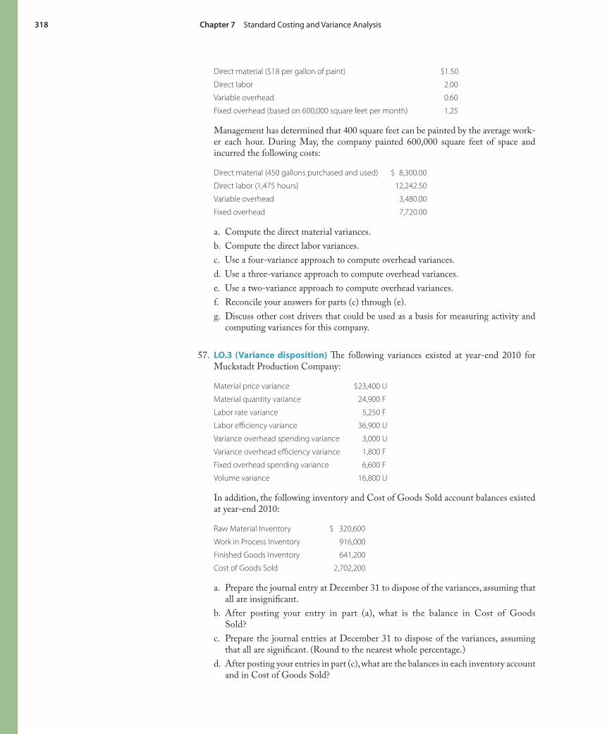
318 Chapter 7 Standard Costing and Variance Analysis
Direct material ($18 per gallon of paint) $1.50
Direct labor 2.00
Variable overhead 0.60
Fixed overhead (based on 600,000 square feet per month) 1.25
Management has determined that 400 square feet can be painted by the average work-er each hour. During May, the company painted 600,000 square feet of space and incurred the following costs:
Direct material (450 gallons purchased and used) $ 8,300.00
Direct labor (1,475 hours) 12,242.50
Variable overhead 3,480.00
Fixed overhead 7,720.00
a. Compute the direct material variances.
b. Compute the direct labor variances.
c. Use a four-variance approach to compute overhead variances.
d. Use a three-variance approach to compute overhead variances.
e. Use a two-variance approach to compute overhead variances.
f. Reconcile your answers for parts (c) through (e).
g. Discuss other cost drivers that could be used as a basis for measuring activity and computing variances for this company.
57. LO.3 (Variance disposition) Th e following variances existed at year-end 2010 for Muckstadt Production Company:
Material price variance $23,400 U
Material quantity variance 24,900 F
Labor rate variance 5,250 F
Labor effi ciency variance 36,900 U
Variance overhead spending variance 3,000 U
Variance overhead effi ciency variance 1,800 F
Fixed overhead spending variance 6,600 F
Volume variance 16,800 U
In addition, the following inventory and Cost of Goods Sold account balances existed at year-end 2010:
Raw Material Inventory $ 320,600
Work in Process Inventory 916,000
Finished Goods Inventory 641,200
Cost of Goods Sold 2,702,200
a. Prepare the journal entry at December 31 to dispose of the variances, assuming that all are insignifi cant.
b. After posting your entry in part (a), what is the balance in Cost of Goods Sold?
c. Prepare the journal entries at December 31 to dispose of the variances, assuming that all are signifi cant. (Round to the nearest whole percentage.)
d. After posting your entries in part (c), what are the balances in each inventory account and in Cost of Goods Sold?

Chapter 7 Standard Costing and Variance Analysis 319
58. LO.3 (Variances and variance responsibility) Namathe Industries manufactures children’s footballs with the following standard costs per unit:
Material: one square foot of leather at $2.00 $ 2.00
Direct labor: 1.6 hours at $9.00 14.40
Variable overhead cost 3.00
Fixed overhead cost 3.00
Total cost per unit $22.40
Per-unit overhead cost was calculated from the following annual overhead budget for 180,000 footballs.
Variable Overhead Cost
Indirect labor—90,000 hours at $7.00 $630,000
Supplies (oil)—180,000 gallons at $0.50 90,000
Allocated variable service department costs 90,000
Total variable overhead cost $ 810,000
Fixed Overhead Cost
Supervision $ 81,000
Depreciation 135,000Other fi xed costs 45,000
Total fi xed overhead cost 261,000
Total budgeted overhead cost at 180,000 units $1,071,000
Following are the charges to the manufacturing department for November when 15,000 units were produced:
Material (15,900 square feet at $2.00) $ 31,800
Direct labor (24,600 hours at $9.10) 223,860
Indirect labor (7,200 hours at $7.10) 51,120
Supplies (oil) (18,000 gallons at $0.55) 9,900
Allocated service department variable OH costs 9,600
Supervision 7,425
Depreciation 11,250
Other fi xed costs 3,750
Total $348,705
Purchasing normally buys about the same quantity as is used in production during a month. In November, the company purchased 15,600 square feet of material at a price of $2.10 per foot.
a. Calculate the following variances from standard costs for the data given:
1. Material purchase price
2. Material quantity
3. Direct labor rate
4. Direct labor effi ciency
5. Overhead budget
b. Th e company has divided its responsibilities so that the Purchasing Department is responsible for the purchase price of materials and the Manufacturing Department is responsible for the quantity of materials used. Does this division of responsibili-ties solve the confl ict between price and quantity variances? Explain your answer.

320 Chapter 7 Standard Costing and Variance Analysis
c. Prepare a report detailing the overhead budget variance. Th e report, which will be given to the Manufacturing Department manager, should only show that part of the variance which is her responsibility and should highlight the information in ways that would be useful to her in evaluating departmental performance and when considering corrective action.
d. Assume that the departmental manager performs the timekeeping function for this manufacturing department. From time to time, analyses of overhead and direct labor variances have shown that the manager has deliberately misclassifi ed labor hours (i.e., listed direct labor hours as indirect labor hours and vice versa) so that only one of the two labor variances is unfavorable. It is not feasible economically to hire a separate timekeeper. What should the company do, if anything, to resolve this problem?
59. LO.4 (Standards revision; writing) Ripper Corp. uses a standard cost system for its aircraft component manufacturing operations. Recently, the company’s direct material supplier went out of business, but Ripper’s purchasing agent found a new source that produces a similar material. Th e price per pound from the original supplier was $7.00; the new source’s price is $7.77. Th e new source’s material reduces scrap and, thus, each unit requires only 1.00 pound rather than the previous standard of 1.25 pounds per unit. In addition, use of the new source’s material reduces direct labor time from 24 to 22 minutes per unit because there is less machine setup time. At the same time, the recently signed labor contract increased the average direct labor wage rate from $12.60 to $14.40 per hour.
Th e company began using the new direct material on April 1, the same day that the new labor agreement went into eff ect. However, Ripper Corp. is still using the follow-ing standards that were set at the beginning of the calendar year:
Direct material 1.2 pounds at $6.80 per pound $ 8.16
Direct labor 20 minutes at $12.30 per DLH 4.10
Standard DM and DL cost per unit $12.26
Steve Wenskel, cost accounting supervisor, had been examining the following April 30 variance report.
PERFORMANCE REPORT STANDARD COST VARIANCE ANALYSIS FOR APRIL 2010
Standard Price Variance Quantity Variance Actual
DM $ 8.16 ($0.97 � 1.0) $0.97 U ($6.80 � 0.2) $1.36 F $ 7.77
DL 4.10 [$2.10 � (22/60)] 0.77 U [$12.30 � (2/60)] 0.41 U 5.28
$12.26 $13.05
COMPARISON OF 2010 ACTUAL COSTS
Average 1st Quarter Costs April Costs Percent Increase (Decrease)
DM $ 8.75 $ 7.77 (11.2)
DL 5.04 5.28 4.8
$13.79 $13.05 (5.4)
When Cynthia Dirope, assistant controller, came into Wenskel’s office, he said, “Cynthia, look at this performance report! Direct material price increased 11 per-cent, and the labor rate increased over 14 percent during April. I expected greater variances, yet prime costs decreased over 5 percent from the $13.79 we experi-enced during the first quarter of this year. The proper message just isn’t coming through.”

Chapter 7 Standard Costing and Variance Analysis 321
Dirope said, “Th is has been an unusual period. With all the unforeseen changes, perhaps we should revise our standards based on current conditions and start over.”
Wenskel replied, “I think we can retain the current standards but expand the vari-ance analysis. We could calculate variances for the specifi c changes that have occurred to direct material and direct labor before we calculate the normal price and quantity vari-ances. What I really think would be useful to management right now is to determine the impact the changes in direct material and direct labor had in reducing our prime costs per unit from $13.79 in the fi rst quarter to $13.05 in April—a reduction of $0.74.”
a. Discuss the advantages of (1) immediately revising the standards and (2) retaining the current standards and expanding the analysis of variances.
b. Prepare an analysis that refl ects the impact of the new direct material and new labor contract on reducing Ripper Corp.’s standard costs per unit from $13.79 to $13.05. Th e analysis should show the changes in direct material and direct labor costs per unit that are caused by (1) the use of the new direct material and (2) the labor rates of the new contract. Th is analysis should be in suffi cient detail to identify the changes due to direct material price, direct labor rate, the eff ect of direct material quality on direct material usage, and the eff ect of direct material quality on direct labor usage.
60. LO.5 (Conversion cost variances) Th e May budget for the Auberage Company shows $1,080,000 of variable conversion costs, $360,000 of fi xed conversion costs, and 72,000 machine hours for the production of 24,000 units of product. During May, 76,000 machine hours were worked and 24,000 units were produced. Variance and fi xed conversion costs for the month were $1,128,800 and $374,500, respectively.
a. Calculate the four conversion cost variances assuming that variable and fi xed costs are separated.
b. Calculate the three conversion cost variances assuming that fi xed and variable costs are combined.
61. LO.5 (Conversion cost variances) Kieff er Company makes men’s suit alterations for a major clothing store chain. No direct materials are used in the alterations process and overhead costs are primarily variable and relate very closely to direct labor charges. Th e company owner has decided to compute variances on a conversion cost basis. Standards for 2010 are as follows:
Expected direct labor hours (DLHs; to be incurred evenly throughout the year) 60,000
Number of suits altered in October 1,800
Standard DLHs per suit 3
Actual DLHs worked in October 2010 5,490
Budgeted variable conversion cost per DLH $ 18
Budgeted annual fi xed conversion cost $ 72,000
Actual variable conversion cost for October 2010 $103,100
Actual fi xed conversion cost for October 2010 $ 5,750
a. How many suits does Kieff er Company expect to alter during 2010?
b. What is the predetermined fi xed OH rate for Kieff er Company?
c. How many standard direct labor hours were allowed for October 2010?
d. Calculate the four conversion cost variances assuming that variable and fi xed costs are separated.
e. Calculate the three conversion cost variances assuming that fi xed and variable costs are combined.

322 Chapter 7 Standard Costing and Variance Analysis
62. LO.6 (Appendix) Polermo Inc. produces three-topping, 18-inch frozen pizzas and uses a standard cost system. Th e three pizza toppings (in addition to cheese) are onions, olives, and mushrooms. To some extent, discretion may be used to determine the actual mix of these toppings. Th e company has two classes of labor, and discretion also may be used to determine the mix of the labor inputs. Th e standard cost card for a pizza follows:
Onions 3 ounces at $0.10 per ounce
Olives 3 ounces at $0.35 per ounce
Mushrooms 3 ounces at $0.50 per ounce
Labor category 1 5 minutes at $12 per hour
Labor category 2 6 minutes at $8 per hour
During May 2010, the company produced 48,000 pizzas and used the following inputs:
Onions 8,000 pounds
Olives 12,000 pounds
Mushrooms 8,000 pounds
Labor category 1 5,200 hours
Labor category 2 4,000 hours
During the month there were no deviations from standards on material prices or labor rates.
a. Determine the material quantity, mix, and yield variances.
b. Determine the labor effi ciency, mix, and yield variances.
c. Prepare the journal entries to record the above mix and yield variances.
63. LO.6 (Appendix) Haddas Ltd. makes Healthy Life, a nutritional aid. For a 50-pound batch, standard material and labor costs are as follows:
Quantity Unit Price Total
Wheat 25.0 pounds $0.20 per pound $5.00
Barley 25.0 pounds 0.10 per pound 2.50
Corn 10.0 pounds 0.05 per pound 0.50
Skilled labor 0.8 hour 12.00 per hour 9.60
Unskilled labor 0.2 hour 8.00 per hour 1.60
During June, the following materials and labor were used in producing 600 batches of Healthy Life:
Wheat 18,000 pounds at $0.22 per pound
Barley 14,000 pounds at $0.11 per pound
Corn 10,000 pounds at $0.07 per pound
Skilled labor 400 hours at $12.25 per hour
Unskilled labor 260 hours at $9.00 per hour
a. Calculate the material quantity, mix, and yield variances.
b. Calculate the labor effi ciency, mix, and yield variances.