Embed Size (px)
Citation preview
Chapter 7 Use of crop residues and straw
CHAPTER 7 USE OF CROP RESIDUES AND STRAW
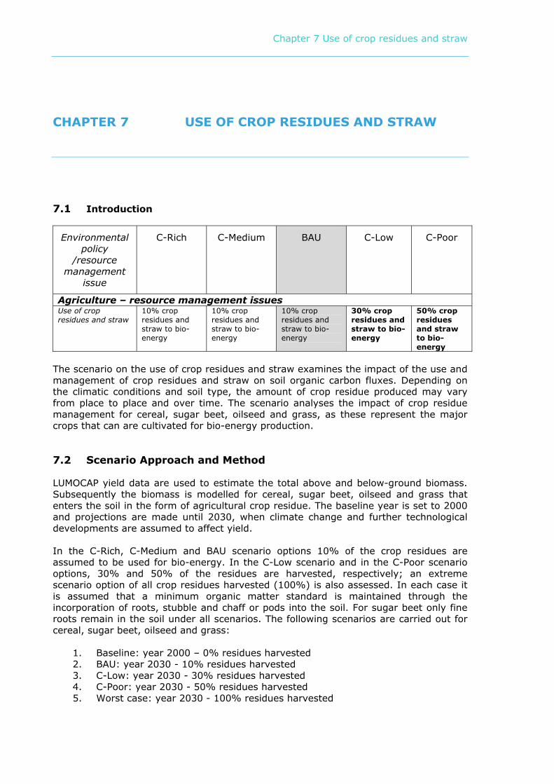
7.1 Introduction
Environmental policy
/resource management
issue
C-Rich C-Medium BAU C-Low C-Poor
Agriculture – resource management issues Use of crop residues and straw
10% crop residues and straw to bio-energy
10% crop residues and straw to bio-energy
10% crop residues and straw to bio-energy
30% crop residues and straw to bio-energy
50% crop residues and straw to bio-energy
The scenario on the use of crop residues and straw examines the impact of the use and management of crop residues and straw on soil organic carbon fluxes. Depending on the climatic conditions and soil type, the amount of crop residue produced may vary from place to place and over time. The scenario analyses the impact of crop residue management for cereal, sugar beet, oilseed and grass, as these represent the major crops that can are cultivated for bio-energy production.
7.2 Scenario Approach and Method
LUMOCAP yield data are used to estimate the total above and below-ground biomass. Subsequently the biomass is modelled for cereal, sugar beet, oilseed and grass that enters the soil in the form of agricultural crop residue. The baseline year is set to 2000 and projections are made until 2030, when climate change and further technological developments are assumed to affect yield. In the C-Rich, C-Medium and BAU scenario options 10% of the crop residues are assumed to be used for bio-energy. In the C-Low scenario and in the C-Poor scenario options, 30% and 50% of the residues are harvested, respectively; an extreme scenario option of all crop residues harvested (100%) is also assessed. In each case it is assumed that a minimum organic matter standard is maintained through the incorporation of roots, stubble and chaff or pods into the soil. For sugar beet only fine roots remain in the soil under all scenarios. The following scenarios are carried out for cereal, sugar beet, oilseed and grass:
1. Baseline: year 2000 – 0% residues harvested 2. BAU: year 2030 - 10% residues harvested 3. C-Low: year 2030 - 30% residues harvested 4. C-Poor: year 2030 - 50% residues harvested 5. Worst case: year 2030 - 100% residues harvested
Chapter 7 Use of crop residues and straw
The following steps are taken in the analysis:
1. LUMOCAP yield data are used to estimate the total above and below-ground biomass for cereal, sugar beet, oilseed and grass for the baseline 2000 and 2030; 2. REGSOM uses crop harvest indices (HI) to determine the above-ground crop biomass and crop root:shoot ratios (RSR) to determine below-ground crop biomass. The total crop biomass generated by a crop equals the above ground plus the below-ground crop biomass. A humification function is then included to derive humified organic carbon (HOC) per hectare. The relevant parameters for these terms for cereal, sugar beet, oilseed and grass are listed in Table 1. 3. REGSOM derives humified organic carbon (HOC) per hectare maps for each of the specified scenarios to compare the impact of different resource management options on regional soil organic carbon fluxes from crop residues and straw.
7.3 Regional organic matter balance for crop residues
Agricultural potential for organic matter sources depends on residue production such as crop residues from annual and perennial crops and manure application. Agriculture in Europe has a high technical potential for biomass production. In particular cereal straw, which is most often returned to the soil in arable cropping systems, is of renewed interest as a potential source of bio-energy. However, the sustainability of this practice which implies systematic removal of above ground biomass of cereal crops is a controversial issue, particularly in soils already having a low soil organic carbon content. We have therefore concentrated on calculating the regional organic matter balance for cereal production across EU-27. The biomass and organic matter potential from crop production is derived from cultivated area and crop yield. Biomass production data are census data available from the Farm Structure Survey (Eurostat) and have been coupled to land use from the Corine Land Cover map. The year 2000 is used as the baseline by the LUMOCAP model. The LUMOCAP model projects future crop yields for cereals, rice, oilseeds, sugar beet, potatoes, fodder, tobacco, vegetables, grass, fruit, vineyards and olives (for more information see Annex I). The harvest index (HI in Table 1) of the crop, i.e. the ratio of harvested product such as grain to above-ground crop biomass, determines the amount of above-ground crop residues. The root:shoot ratio (RSR in Table 1) determines the below-ground crop biomass. The total crop biomass generated by a crop equals the sum of the above-ground and below-ground biomass. For tuber crops, the harvest index is the ratio of tuber harvested to the below-ground biomass and the root:shoot ratio determines the above-ground biomass that is regarded as crop residue. Different crop varieties will have different values for HI. The amount of total residue produced will vary from year to year depending on variations in inter alia weather, water availability, soil fertility and farming practices. The rooting system, root:shoot ratio and residue management ultimately determine the level of agricultural crop residue that can be left on the field to contribute to soil organic matter. The residue left on the field equals the total crop biomass, both above ground and below ground, minus the harvested products. For cereals the harvested products may be grain and straw. The residues can be calculated using the harvest index, the root:shoot ratio and the yield.
H = R.(e-Akt) where R is the amount of residue added to the soil, expressed in tonnes C/ha, with 0.5 as C:OM ratio. H is the amount of organic carbon that humifies after one year. k is the
Chapter 7 Use of crop residues and straw
decay factor or humification rate (Table 11) and t is year. In subsequent modelling steps k is corrected for temperature, moisture and plant development (A); and different decay rates (k) are introduced per organic matter compartment.
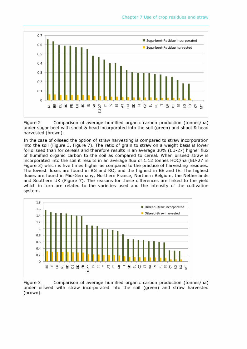
Table 1 Average crop parameters for organic matter production on agricultural land
Crop parameters Crop Harvest
Indices (HI)
Root-Shoot Ratio (RSR in DM)
Humification rate (k in year-1)
C:OM
Cereal 0.62 0.41 0.31 0.5 Sugar beet 0.99 14.29 0.29 0.5 Oilseed 0.29 0.18 0.31 0.5 Grass 1.00 0.80 0.26 0.5
Large quantities of residues are generated every year by agriculture. Cereals, grass, sugar beet, potatoes and oilseed rape are arable crops that generate considerable amounts of residues. In aggregate, figures of the total amount of residues look very attractive if not staggering. A distinction, however, has to be made between residues remaining in the field and those generated after harvesting and during processing. Field residues occur in smaller quantities, are spread over large(r) areas and remain in the field; examples are stubble, straw, stalks and leaves depending on the crop and the farming practice. Biomass and harvested residues are used for many often site-specific purposes: food, fodder, feedstock, fibre, fuel and further use such as compost production. These purposes are often not mutually exclusive; for example, straw can be used as animal bedding and thereafter as fertiliser. After processing residues can be concentrated which make their further use for compost production and soil amelioration easier. Agricultural field residues constitute a major part of the total annual production of biomass and the residues are an important source of soil organic matter. The biomass residues that effectively contribute to the soil organic matter stock depend on the effective organic matter or the amount of organic matter left after one year of decay. Roughly this will be 25% of the freshly introduced organic material left on site, but for each crop the decay rates are different. Depending on the decay rates, the effective organic matter will be converted to stable humified organic matter. We converted the humified organic matter to humified organic carbon (HOC) assuming a 50% ratio of carbon to organic matter. The data on harvest indices, root/shoot ratios and effective organic carbon content are combined with cropping areas and crop production such that the amount of agricultural residues generated can be calculated. The yield data are extracted from the LUMOCAP framework and rely on national and international statistics collected by Eurostat. The LUMOCAP framework, however, does not make a distinction between irrigated and non-irrigated crops such that yield and therefore organic matter input in Mediterranean areas may be overestimated. The meteorological influence in these regions, however, assumes a hot and dry environment for decay of the organic matter input. We compared two residue management options for cereals, sugar beet and oilseed (described below). For both options we assumed that roots, stubble and chaff (cereal); roots, stubble and pods (oilseed) or fine roots (sugar beet) were left as residue on the field. For permanent grassland we assumed productive grassland with regular harvesting, i.e. yearly removal of biomass. For comparison, we also assumed the hypothetical practice of ploughing all grass biomass into the soil, a practice which is
Chapter 7 Use of crop residues and straw
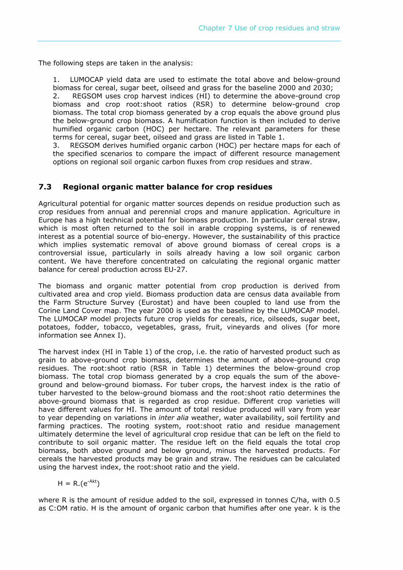
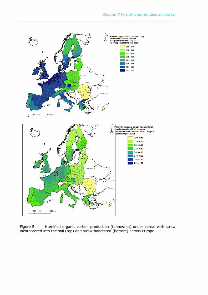
common to temporary grassland. We also assumed that all other residues left the field and did not return in another form (e.g. compost). The amount of humified organic carbon added to the soil depends first of all on the yields as these directly relate to residue, and secondly on the prevailing climate with cold temperatures and dry moisture regimes being less favourable. For cereal production two extreme management options are presented: straw left as residue on the field and straw harvested (Figure 1, Figure 5). The practice of leaving cereal straw in the field has the potential of doubling the effective organic matter input. Member States with a high production such as BE, NL, IE, DK, UK, DE, LU and FR have a higher potential for sequestering carbon into the soil than the average for EU-27 at 0.86 tonnes/ha for all straw incorporated and at 0.44 tonnes carbon/ha for all straw harvested (Figure 1). The regional distribution further confirms this with southeast UK, Northern France, Northern Belgium, the Netherlands and Northern Germany displaying the largest humified organic carbon input of Europe (Figure 5).
0.000
0.200
0.400
0.600
0.800
1.000
1.200
1.400
BE NL IE DK
UK DE
LU FR SE
EU-2
7 ES IT PT GR AT FI LT SK HU CZ SL LV PL EE MT CY RO BG
Cereal-Straw Incorporated
Cereal-Straw harvested
Figure 1 Comparison of average humified organic carbon production (tonnes/ha) under cereal with straw incorporated into the soil (green) and straw harvested (yellow).
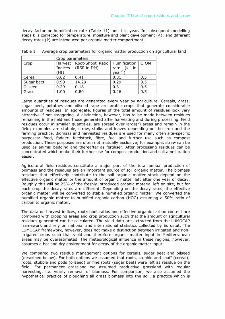
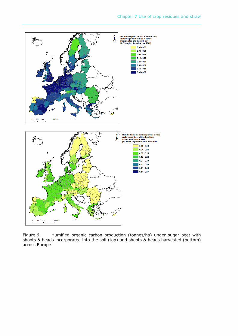
Sugar beet only has half of the capacity for adding humified organic carbon (HOC) to the soil as compared to cereal. This is due to a large harvest index and large root:shoot ratio, leaving little residue on the field as compared to cereals. For sugar beet production the option of shoots incorporated into the soil is compared to combined root and shoot harvesting (Figure 2, Figure 6). Although the potential to introduce organic matter into the soil is lower as compared to cereals, residue management has a large impact. Root and shoot harvesting leaves little organic matter after cultivation: with an EU-27 average of 0.046 tonnes HOC/ha a factor 10 less as compared to residue incorporation into the soil (Figure 2), which is also reflected in maps presenting the regional distribution (Figure 6).
Chapter 7 Use of crop residues and straw
0
0.1
0.2
0.3
0.4
0.5
0.6
0.7
NL
BE DE
DK FR LU UK IE GR
EU-2
7 IT ES SE AT
HU SK FI CZ SL PL LT LV PT EE BG RO CY MT
Sugarbeet-Residue Incorporated
Sugarbeet-Residue harvested
Figure 2 Comparison of average humified organic carbon production (tonnes/ha) under sugar beet with shoot & head incorporated into the soil (green) and shoot & head harvested (brown).
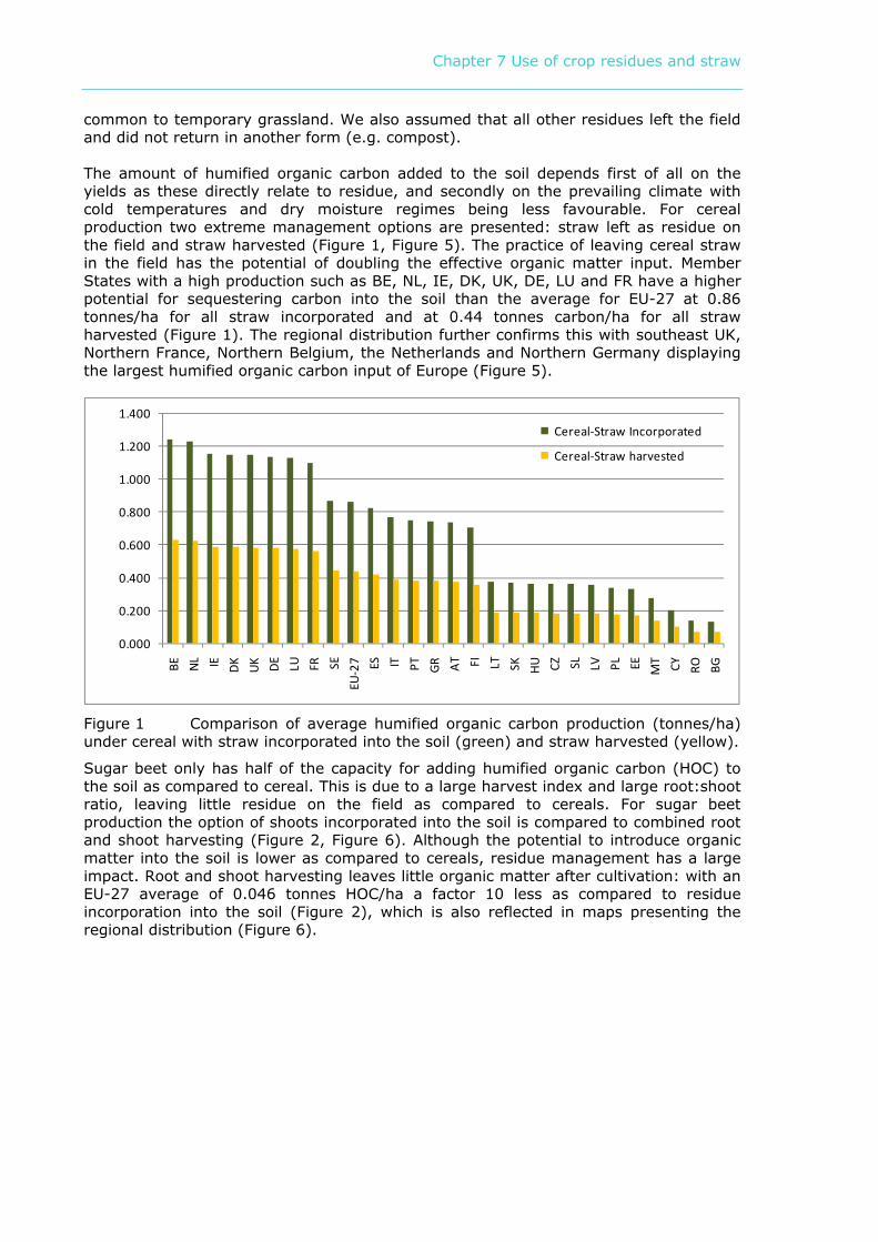
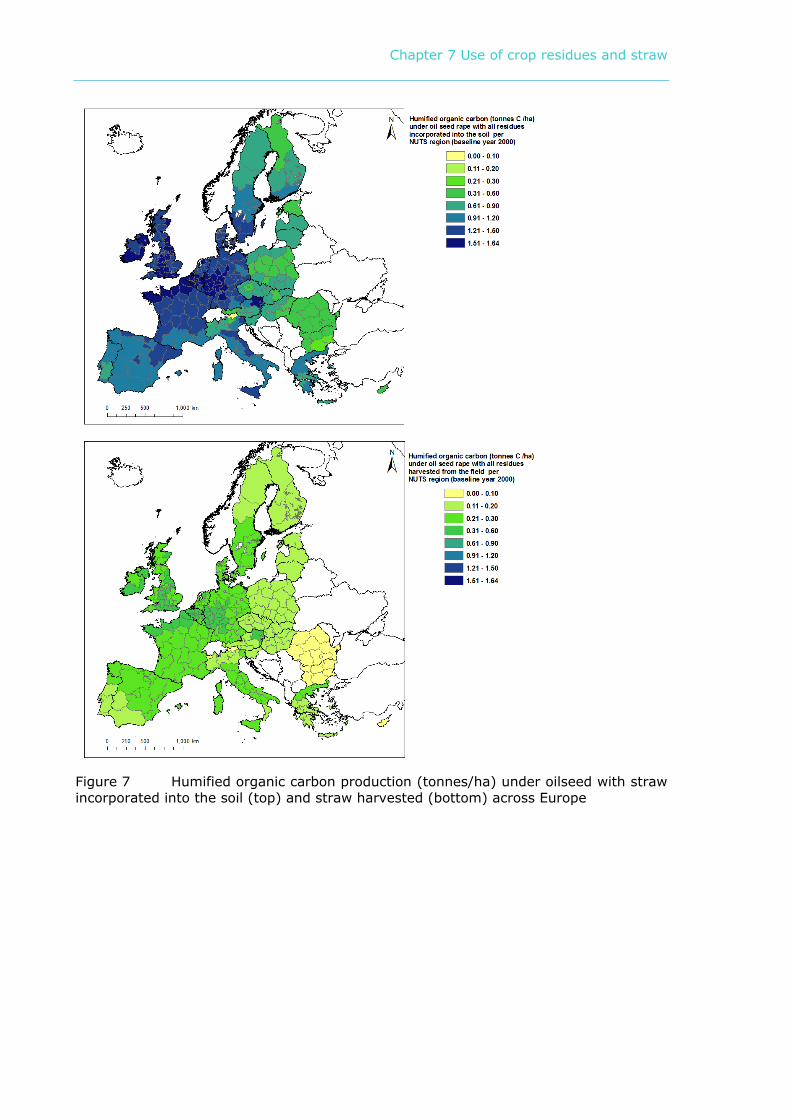
In the case of oilseed the option of straw harvesting is compared to straw incorporation into the soil (Figure 3, Figure 7). The ratio of grain to straw on a weight basis is lower for oilseed than for cereals and therefore results in an average 30% (EU-27) higher flux of humified organic carbon to the soil as compared to cereal. When oilseed straw is incorporated into the soil it results in an average flux of 1.12 tonnes HOC/ha (EU-27 in Figure 3) which is five times higher as compared to the practice of harvesting residues. The lowest fluxes are found in BG and RO, and the highest in BE and IE. The highest fluxes are found in Mid-Germany, Northern France, Northern Belgium, the Netherlands and Southern UK (Figure 7). The reasons for these differences are linked to the yield which in turn are related to the varieties used and the intensity of the cultivation system.
0
0.2
0.4
0.6
0.8
1
1.2
1.4
1.6
1.8
BE IE LU NL
UK DE
DK FR
EU-2
7 ES SE IT AT
PT GR FI SK SL CZ LT HU LV PL EE CY RO BG MT
Oilseed-Straw Incorporated
Oilseed-Straw harvested
Figure 3 Comparison of average humified organic carbon production (tonnes/ha) under oilseed with straw incorporated into the soil (green) and straw harvested (brown).
Chapter 7 Use of crop residues and straw
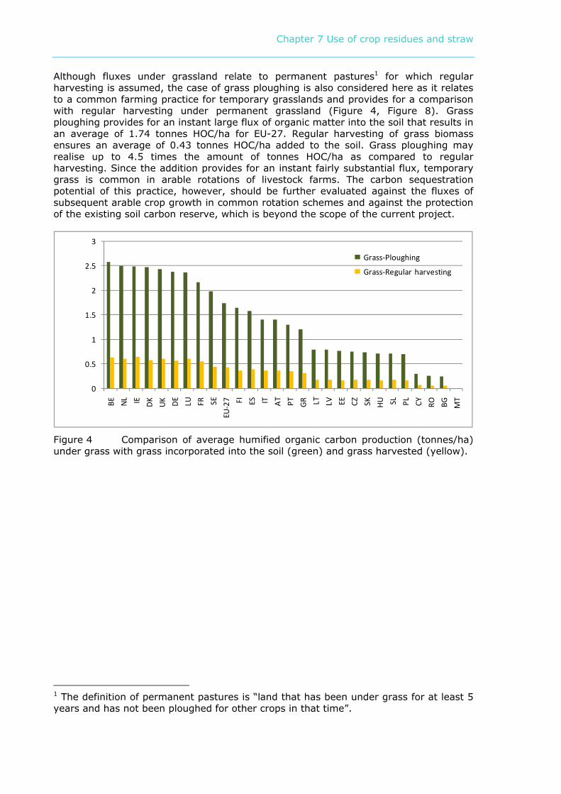
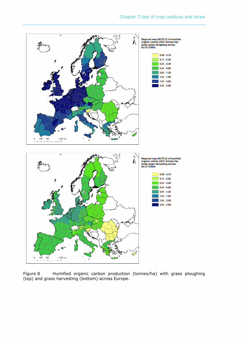
Although fluxes under grassland relate to permanent pastures1 for which regular harvesting is assumed, the case of grass ploughing is also considered here as it relates to a common farming practice for temporary grasslands and provides for a comparison with regular harvesting under permanent grassland (Figure 4, Figure 8). Grass ploughing provides for an instant large flux of organic matter into the soil that results in an average of 1.74 tonnes HOC/ha for EU-27. Regular harvesting of grass biomass ensures an average of 0.43 tonnes HOC/ha added to the soil. Grass ploughing may realise up to 4.5 times the amount of tonnes HOC/ha as compared to regular harvesting. Since the addition provides for an instant fairly substantial flux, temporary grass is common in arable rotations of livestock farms. The carbon sequestration potential of this practice, however, should be further evaluated against the fluxes of subsequent arable crop growth in common rotation schemes and against the protection of the existing soil carbon reserve, which is beyond the scope of the current project.
0
0.5
1
1.5
2
2.5
3
BE NL IE DK
UK DE
LU FR SE
EU-2
7 FI ES IT AT
PT GR LT LV EE CZ SK HU SL PL CY RO BG MT
Grass-Ploughing
Grass-Regular harvesting
Figure 4 Comparison of average humified organic carbon production (tonnes/ha) under grass with grass incorporated into the soil (green) and grass harvested (yellow).
1 The definition of permanent pastures is “land that has been under grass for at least 5 years and has not been ploughed for other crops in that time”.
Chapter 7 Use of crop residues and straw
Figure 5 Humified organic carbon production (tonnes/ha) under cereal with straw incorporated into the soil (top) and straw harvested (bottom) across Europe
Chapter 7 Use of crop residues and straw
Figure 6 Humified organic carbon production (tonnes/ha) under sugar beet with shoots & heads incorporated into the soil (top) and shoots & heads harvested (bottom) across Europe
Chapter 7 Use of crop residues and straw
Figure 7 Humified organic carbon production (tonnes/ha) under oilseed with straw incorporated into the soil (top) and straw harvested (bottom) across Europe
Chapter 7 Use of crop residues and straw
Figure 8 Humified organic carbon production (tonnes/ha) with grass ploughing (top) and grass harvesting (bottom) across Europe.
Chapter 7 Use of crop residues and straw
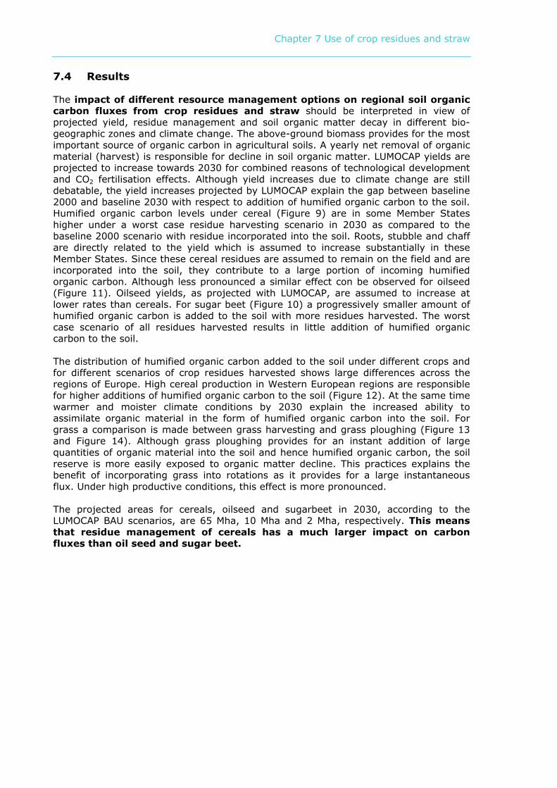
7.4 Results
The impact of different resource management options on regional soil organic carbon fluxes from crop residues and straw should be interpreted in view of projected yield, residue management and soil organic matter decay in different bio-geographic zones and climate change. The above-ground biomass provides for the most important source of organic carbon in agricultural soils. A yearly net removal of organic material (harvest) is responsible for decline in soil organic matter. LUMOCAP yields are projected to increase towards 2030 for combined reasons of technological development and CO2 fertilisation effects. Although yield increases due to climate change are still debatable, the yield increases projected by LUMOCAP explain the gap between baseline 2000 and baseline 2030 with respect to addition of humified organic carbon to the soil. Humified organic carbon levels under cereal (Figure 9) are in some Member States higher under a worst case residue harvesting scenario in 2030 as compared to the baseline 2000 scenario with residue incorporated into the soil. Roots, stubble and chaff are directly related to the yield which is assumed to increase substantially in these Member States. Since these cereal residues are assumed to remain on the field and are incorporated into the soil, they contribute to a large portion of incoming humified organic carbon. Although less pronounced a similar effect con be observed for oilseed (Figure 11). Oilseed yields, as projected with LUMOCAP, are assumed to increase at lower rates than cereals. For sugar beet (Figure 10) a progressively smaller amount of humified organic carbon is added to the soil with more residues harvested. The worst case scenario of all residues harvested results in little addition of humified organic carbon to the soil. The distribution of humified organic carbon added to the soil under different crops and for different scenarios of crop residues harvested shows large differences across the regions of Europe. High cereal production in Western European regions are responsible for higher additions of humified organic carbon to the soil (Figure 12). At the same time warmer and moister climate conditions by 2030 explain the increased ability to assimilate organic material in the form of humified organic carbon into the soil. For grass a comparison is made between grass harvesting and grass ploughing (Figure 13 and Figure 14). Although grass ploughing provides for an instant addition of large quantities of organic material into the soil and hence humified organic carbon, the soil reserve is more easily exposed to organic matter decline. This practices explains the benefit of incorporating grass into rotations as it provides for a large instantaneous flux. Under high productive conditions, this effect is more pronounced. The projected areas for cereals, oilseed and sugarbeet in 2030, according to the LUMOCAP BAU scenarios, are 65 Mha, 10 Mha and 2 Mha, respectively. This means that residue management of cereals has a much larger impact on carbon fluxes than oil seed and sugar beet.
Chapter 7 Use of crop residues and straw
0.00
0.20
0.40
0.60
0.80
1.00
1.20
1.40
1.60
BE NL IE DK UK DE LU FR SE ES EU-27 IT PT GR AT FI LT SK HU CZ SL LV PL EE MT CY RO BG
Cereal-2000-0%
Cereal-2030-0%
Cereal-2030-10%
Cereal-2030-30%
Cereal-2030-50%
Cereal-2030-100%
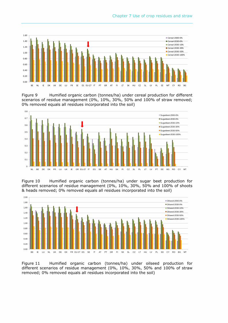
Figure 9 Humified organic carbon (tonnes/ha) under cereal production for different scenarios of residue management (0%, 10%, 30%, 50% and 100% of straw removed; 0% removed equals all residues incorporated into the soil)
0
0.1
0.2
0.3
0.4
0.5
0.6
0.7
0.8
NL BE DE DK FR LU UK IE GR EU-27 IT ES SE AT HU SK FI CZ SL PL LT LV PT EE BG RO CY MT
Sugarbeet-2000-0%
Sugarbeet-2030-0%
Sugarbeet-2030-10%
Sugarbeet-2030-30%
Sugarbeet-2030-50%
Sugarbeet-2030-100%
Figure 10 Humified organic carbon (tonnes/ha) under sugar beet production for different scenarios of residue management (0%, 10%, 30%, 50% and 100% of shoots & heads removed; 0% removed equals all residues incorporated into the soil)
0.00
0.20
0.40
0.60
0.80
1.00
1.20
1.40
1.60
1.80
2.00
BE IE LU NL UK DE DK FR EU-27 ES SE IT AT PT GR FI SK SL CZ LT HU LV PL EE CY RO BG MT
Oilseed-2000-0%
Oilseed-2030-0%
Oilseed-2030-10%
Oilseed-2030-30%
Oilseed-2030-50%
Oilseed-2030-100%
Figure 11 Humified organic carbon (tonnes/ha) under oilseed production for different scenarios of residue management (0%, 10%, 30%, 50% and 100% of straw removed; 0% removed equals all residues incorporated into the soil)
Chapter 7 Use of crop residues and straw
BASELINE 2000: 0% straw removed
BASELINE 2030: 0% straw removed
BAU, C-rich, C-med 2030: 10% straw removed
C-low 2030: 30% straw removed
C-Poor 2030: 50% straw removed
WORST CASE 2030: All straw removed
Legend HOC (tonnes/ha)
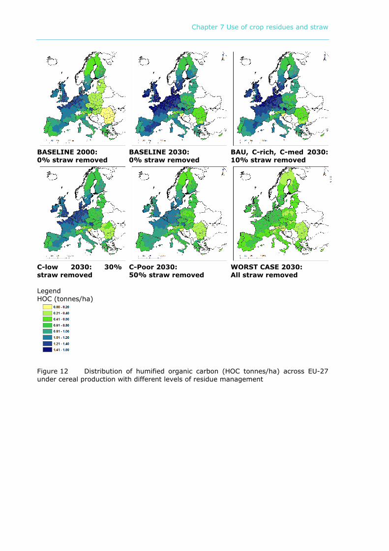
Figure 12 Distribution of humified organic carbon (HOC tonnes/ha) across EU-27 under cereal production with different levels of residue management
Chapter 7 Use of crop residues and straw
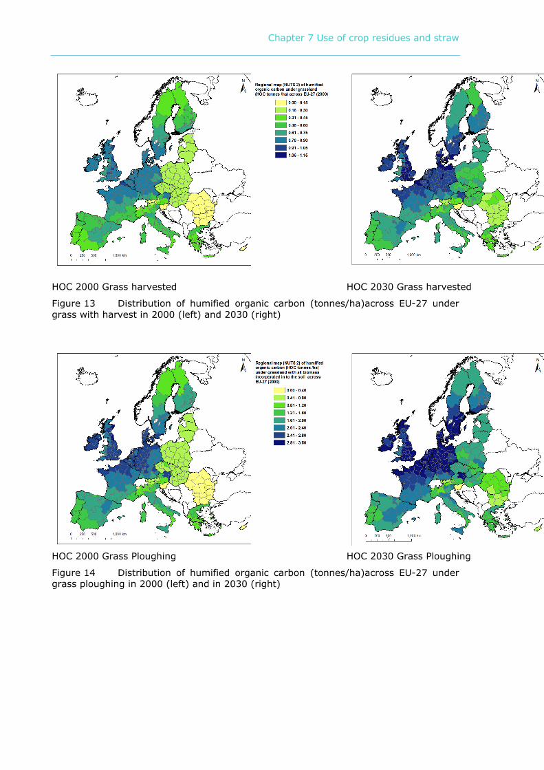
HOC 2000 Grass harvested HOC 2030 Grass harvested
Figure 13 Distribution of humified organic carbon (tonnes/ha)across EU-27 under grass with harvest in 2000 (left) and 2030 (right)
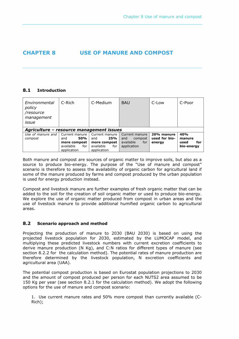
HOC 2000 Grass Ploughing HOC 2030 Grass Ploughing
Figure 14 Distribution of humified organic carbon (tonnes/ha)across EU-27 under grass ploughing in 2000 (left) and in 2030 (right)
Chapter 8 Use of manure and compost
CHAPTER 8 USE OF MANURE AND COMPOST
8.1 Introduction
Environmental policy /resource management issue
C-Rich C-Medium BAU C-Low C-Poor
Agriculture – resource management issues Use of manure and compost
Current manure and 50% more compost available for application
Current manure and 25% more compost available for application
Current manure and compost available for application
20% manure used for bio-energy
40% manure used for bio-energy
Both manure and compost are sources of organic matter to improve soils, but also as a source to produce bio-energy. The purpose of the “Use of manure and compost” scenario is therefore to assess the availability of organic carbon for agricultural land if some of the manure produced by farms and compost produced by the urban population is used for energy production instead. Compost and livestock manure are further examples of fresh organic matter that can be added to the soil for the creation of soil organic matter or used to produce bio-energy. We explore the use of organic matter produced from compost in urban areas and the use of livestock manure to provide additional humified organic carbon to agricultural areas.
8.2 Scenario approach and method
Projecting the production of manure to 2030 (BAU 2030) is based on using the projected livestock population for 2030, estimated by the LUMOCAP model, and multiplying these predicted livestock numbers with current excretion coefficients to derive manure production (N Kg), and C:N ratios for different types of manure (see section 8.2.2 for the calculation method). The potential rates of manure production are therefore determined by the livestock population, N excretion coefficients and agricultural area (UAA). The potential compost production is based on Eurostat population projections to 2030 and the amount of compost produced per person for each NUTS2 area assumed to be 150 Kg per year (see section 8.2.1 for the calculation method). We adopt the following options for the use of manure and compost scenario:
1. Use current manure rates and 50% more compost than currently available (C-Rich);
Chapter 8 Use of manure and compost
2. Use current manure rates and 25% more compost than currently available (C-Medium); 3. Use current manure and compost rates currently available (BAU); 4. Use 20% of manure in 2030 for energy production (C-Low); and, 5. Use 40% of manure in 2030 for energy production (C-Poor).
The following steps are taken in the analysis:
1. Assess the projected trends in livestock manure production and potential compost production; 2. REGSOM derives humified organic carbon (HOC) per hectare maps for each of the specified scenarios to compare the impact of different resource management options on regional soil organic carbon fluxes from livestock manure and potential compost production.
8.2.1 Production of organic matter from urban areas
Households and the service sector (schools, hospitals, offices and shops) are potential providers of compost in urban areas. We calculated compost production in urban areas in two different ways:
1. We used statistics on the different contributors to compost production, i.e. reported compost production; and, 2. We used estimates of compost production based on production rates per capita, which are multiplied by population data to calculate potential compost production in urban areas.
Two types of compost are considered: kitchen compost made from vegetables, fruit and gardening waste (k-compost) and green compost made from made from prunings, branches, grass and leaf litter (G-compost). 8.2.2 Reported compost production
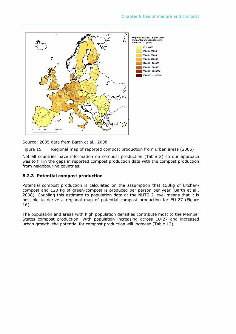
Report compost production is based on data provided by the European Compost Network (Table 12, Barth et al., 2008). We weighted the compost production by population to distribute MS values across the NUTS2 areas per Member State. This results in a map of reported compost production estimates at NUTS2 level (Figure 15).
Chapter 8 Use of manure and compost
Source: 2005 data from Barth et al., 2008
Figure 15 Regional map of reported compost production from urban areas (2005)
Not all countries have information on compost production (Table 2) so our approach was to fill in the gaps in reported compost production data with the compost production from neighbouring countries. 8.2.3 Potential compost production
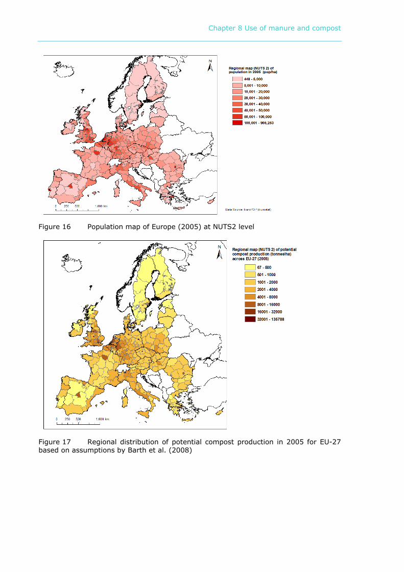
Potential compost production is calculated on the assumption that 150kg of kitchen- compost and 120 kg of green-compost is produced per person per year (Barth et al., 2008). Coupling this estimate to population data at the NUTS 2 level means that it is possible to derive a regional map of potential compost production for EU-27 (Figure 16). The population and areas with high population densities contribute most to the Member States compost production. With population increasing across EU-27 and increased urban growth, the potential for compost production will increase (Table 12).
Chapter 8 Use of manure and compost
Figure 16 Population map of Europe (2005) at NUTS2 level
Figure 17 Regional distribution of potential compost production in 2005 for EU-27 based on assumptions by Barth et al. (2008)
Chapter 8 Use of manure and compost
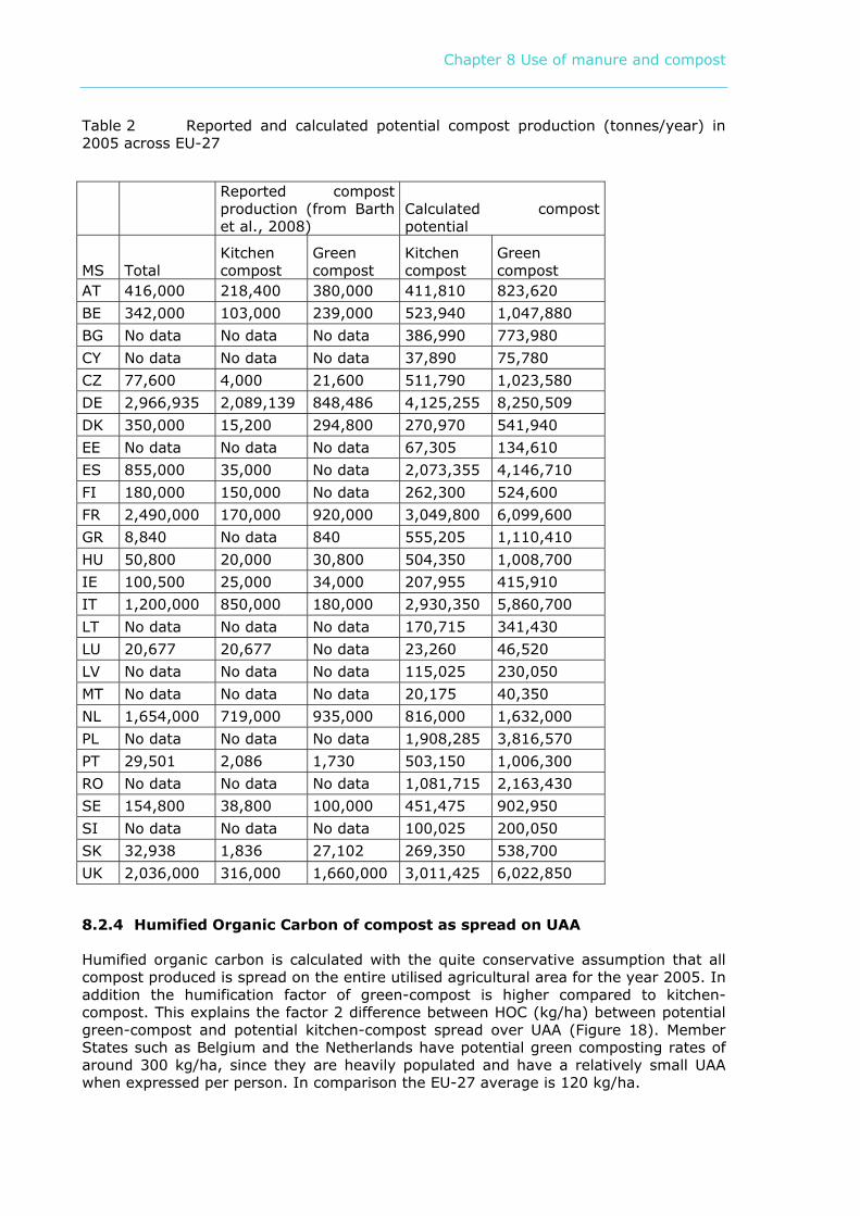
Table 2 Reported and calculated potential compost production (tonnes/year) in 2005 across EU-27
8.2.4 Humified Organic Carbon of compost as spread on UAA
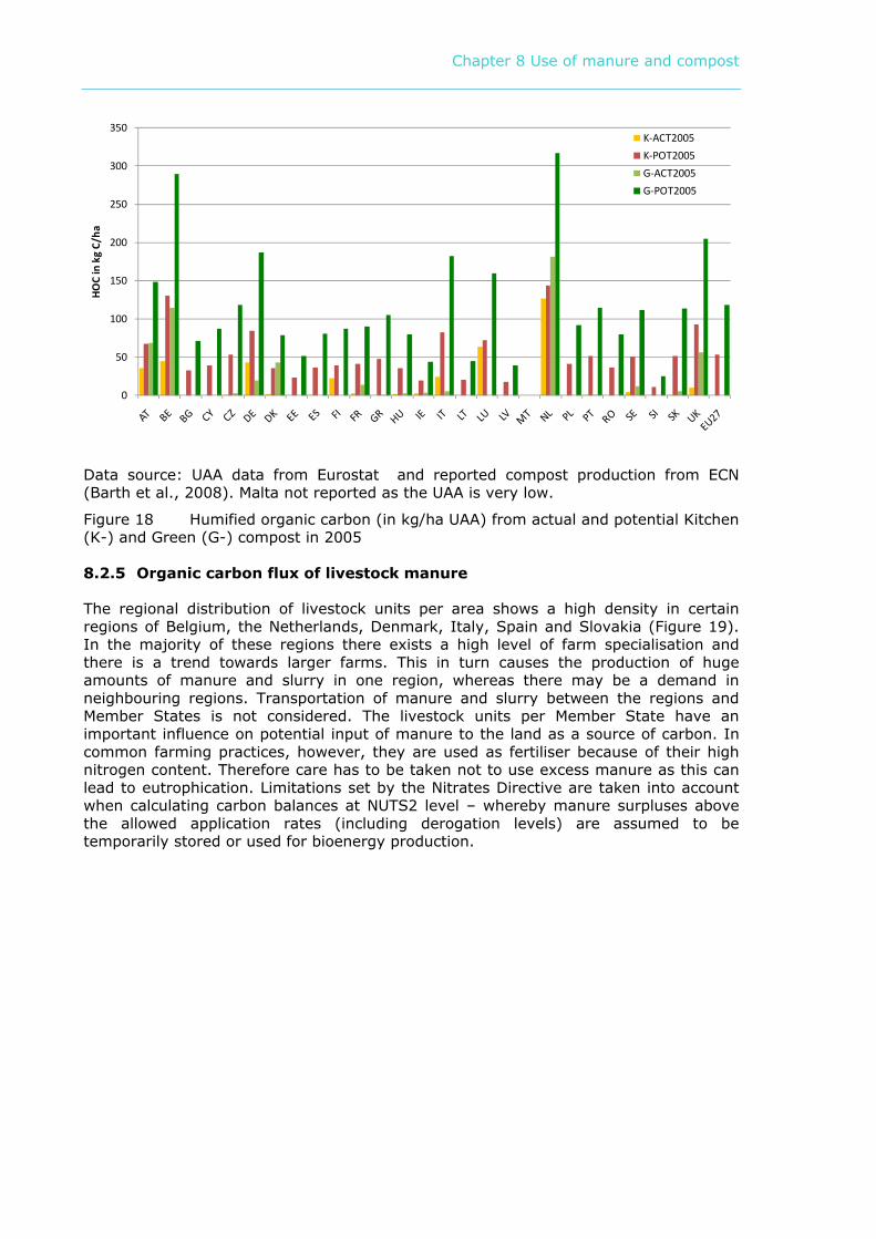
Humified organic carbon is calculated with the quite conservative assumption that all compost produced is spread on the entire utilised agricultural area for the year 2005. In addition the humification factor of green-compost is higher compared to kitchen-compost. This explains the factor 2 difference between HOC (kg/ha) between potential green-compost and potential kitchen-compost spread over UAA (Figure 18). Member States such as Belgium and the Netherlands have potential green composting rates of around 300 kg/ha, since they are heavily populated and have a relatively small UAA when expressed per person. In comparison the EU-27 average is 120 kg/ha.
Reported compost production (from Barth et al., 2008)
Calculated compost potential
MS Total Kitchen compost
Green compost
Kitchen compost
Green compost
AT 416,000 218,400 380,000 411,810 823,620 BE 342,000 103,000 239,000 523,940 1,047,880 BG No data No data No data 386,990 773,980 CY No data No data No data 37,890 75,780 CZ 77,600 4,000 21,600 511,790 1,023,580 DE 2,966,935 2,089,139 848,486 4,125,255 8,250,509 DK 350,000 15,200 294,800 270,970 541,940 EE No data No data No data 67,305 134,610 ES 855,000 35,000 No data 2,073,355 4,146,710 FI 180,000 150,000 No data 262,300 524,600 FR 2,490,000 170,000 920,000 3,049,800 6,099,600 GR 8,840 No data 840 555,205 1,110,410 HU 50,800 20,000 30,800 504,350 1,008,700 IE 100,500 25,000 34,000 207,955 415,910 IT 1,200,000 850,000 180,000 2,930,350 5,860,700 LT No data No data No data 170,715 341,430 LU 20,677 20,677 No data 23,260 46,520 LV No data No data No data 115,025 230,050 MT No data No data No data 20,175 40,350 NL 1,654,000 719,000 935,000 816,000 1,632,000 PL No data No data No data 1,908,285 3,816,570 PT 29,501 2,086 1,730 503,150 1,006,300 RO No data No data No data 1,081,715 2,163,430 SE 154,800 38,800 100,000 451,475 902,950 SI No data No data No data 100,025 200,050 SK 32,938 1,836 27,102 269,350 538,700 UK 2,036,000 316,000 1,660,000 3,011,425 6,022,850
Chapter 8 Use of manure and compost
0
50
100
150
200
250
300
350
HO
C in
kg
C/ha
K-ACT2005
K-POT2005
G-ACT2005
G-POT2005
Data source: UAA data from Eurostat and reported compost production from ECN (Barth et al., 2008). Malta not reported as the UAA is very low.
Figure 18 Humified organic carbon (in kg/ha UAA) from actual and potential Kitchen (K-) and Green (G-) compost in 2005 8.2.5 Organic carbon flux of livestock manure
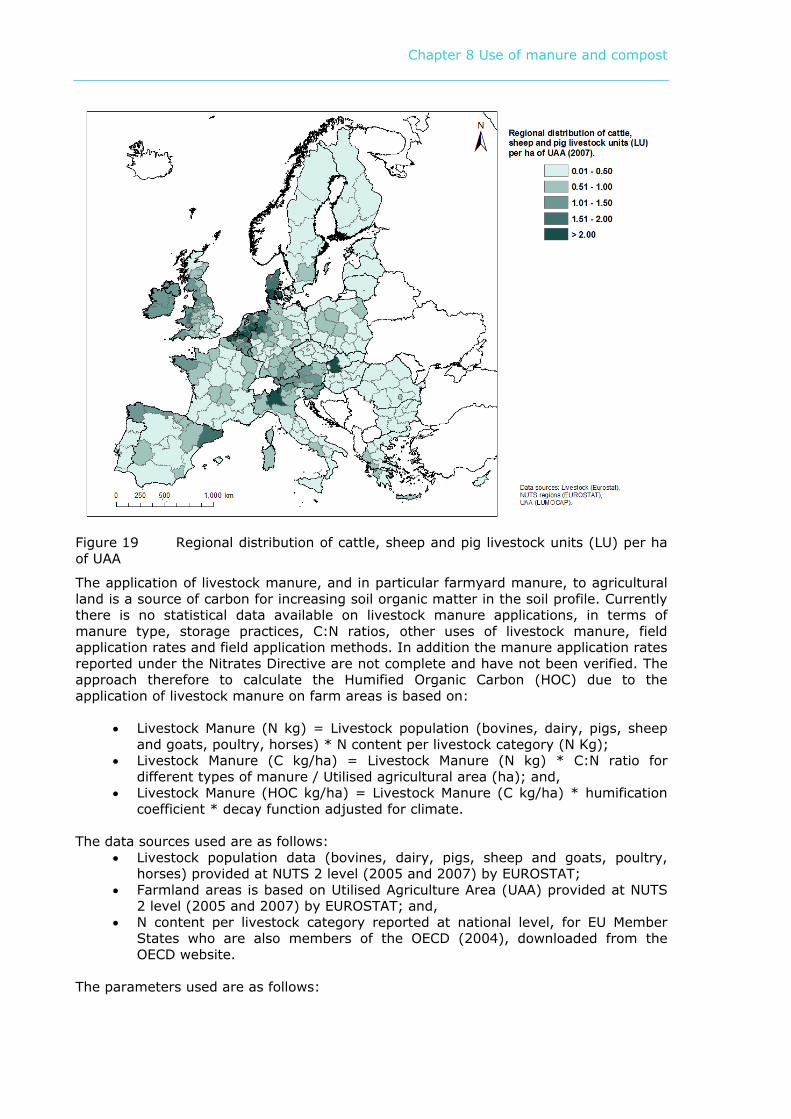
The regional distribution of livestock units per area shows a high density in certain regions of Belgium, the Netherlands, Denmark, Italy, Spain and Slovakia (Figure 19). In the majority of these regions there exists a high level of farm specialisation and there is a trend towards larger farms. This in turn causes the production of huge amounts of manure and slurry in one region, whereas there may be a demand in neighbouring regions. Transportation of manure and slurry between the regions and Member States is not considered. The livestock units per Member State have an important influence on potential input of manure to the land as a source of carbon. In common farming practices, however, they are used as fertiliser because of their high nitrogen content. Therefore care has to be taken not to use excess manure as this can lead to eutrophication. Limitations set by the Nitrates Directive are taken into account when calculating carbon balances at NUTS2 level – whereby manure surpluses above the allowed application rates (including derogation levels) are assumed to be temporarily stored or used for bioenergy production.
Chapter 8 Use of manure and compost
Figure 19 Regional distribution of cattle, sheep and pig livestock units (LU) per ha of UAA
The application of livestock manure, and in particular farmyard manure, to agricultural land is a source of carbon for increasing soil organic matter in the soil profile. Currently there is no statistical data available on livestock manure applications, in terms of manure type, storage practices, C:N ratios, other uses of livestock manure, field application rates and field application methods. In addition the manure application rates reported under the Nitrates Directive are not complete and have not been verified. The approach therefore to calculate the Humified Organic Carbon (HOC) due to the application of livestock manure on farm areas is based on:
• Livestock Manure (N kg) = Livestock population (bovines, dairy, pigs, sheep and goats, poultry, horses) * N content per livestock category (N Kg);
• Livestock Manure (C kg/ha) = Livestock Manure (N kg) * C:N ratio for different types of manure / Utilised agricultural area (ha); and,
• Livestock Manure (HOC kg/ha) = Livestock Manure (C kg/ha) * humification coefficient * decay function adjusted for climate.
The data sources used are as follows: • Livestock population data (bovines, dairy, pigs, sheep and goats, poultry,
horses) provided at NUTS 2 level (2005 and 2007) by EUROSTAT; • Farmland areas is based on Utilised Agriculture Area (UAA) provided at NUTS
2 level (2005 and 2007) by EUROSTAT; and, • N content per livestock category reported at national level, for EU Member
States who are also members of the OECD (2004), downloaded from the OECD website.
The parameters used are as follows:
Chapter 8 Use of manure and compost
• C:N ratio for different types of manure based on fresh weight; • Humification rate to estimate Effective Organic Content; and, • Decay functions related to temperature and moisture.
Not all MS of EU-27 are members of the OECD – so we assume that N content coefficients per livestock category for:
• Estonia, Latvia, Lithuania are the same as Poland; • Bulgaria, Romania, Slovenia are the same as the Czech Republic; and, • Cyprus and Malta are the same as Greece.
N content coefficients can vary between Member States because of differing livestock varieties that have different metabolism and also differing bio-geography. The summary table of N content coefficients (Table 3) indicates that there is a considerable range of N coefficients reported for each livestock category.
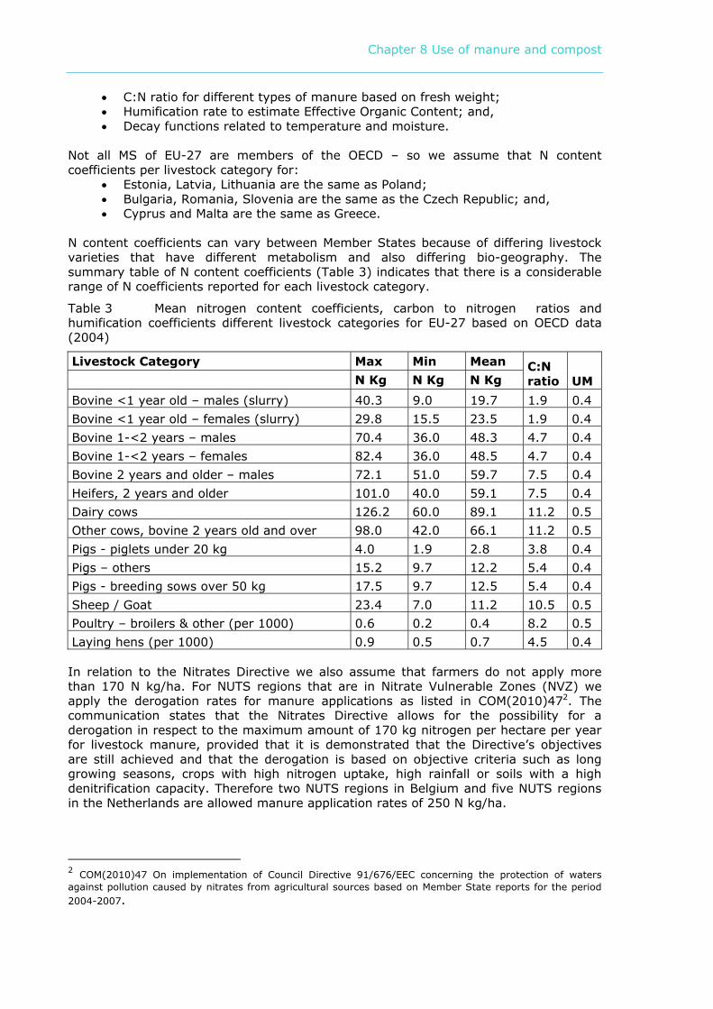
Table 3 Mean nitrogen content coefficients, carbon to nitrogen ratios and humification coefficients different livestock categories for EU-27 based on OECD data (2004)
Livestock Category Max Min Mean
N Kg N Kg N Kg C:N ratio UM
Bovine <1 year old – males (slurry) 40.3 9.0 19.7 1.9 0.4 Bovine <1 year old – females (slurry) 29.8 15.5 23.5 1.9 0.4 Bovine 1-<2 years – males 70.4 36.0 48.3 4.7 0.4 Bovine 1-<2 years – females 82.4 36.0 48.5 4.7 0.4 Bovine 2 years and older – males 72.1 51.0 59.7 7.5 0.4 Heifers, 2 years and older 101.0 40.0 59.1 7.5 0.4 Dairy cows 126.2 60.0 89.1 11.2 0.5 Other cows, bovine 2 years old and over 98.0 42.0 66.1 11.2 0.5 Pigs - piglets under 20 kg 4.0 1.9 2.8 3.8 0.4 Pigs – others 15.2 9.7 12.2 5.4 0.4 Pigs - breeding sows over 50 kg 17.5 9.7 12.5 5.4 0.4 Sheep / Goat 23.4 7.0 11.2 10.5 0.5 Poultry – broilers & other (per 1000) 0.6 0.2 0.4 8.2 0.5 Laying hens (per 1000) 0.9 0.5 0.7 4.5 0.4 In relation to the Nitrates Directive we also assume that farmers do not apply more than 170 N kg/ha. For NUTS regions that are in Nitrate Vulnerable Zones (NVZ) we apply the derogation rates for manure applications as listed in COM(2010)472. The communication states that the Nitrates Directive allows for the possibility for a derogation in respect to the maximum amount of 170 kg nitrogen per hectare per year for livestock manure, provided that it is demonstrated that the Directive’s objectives are still achieved and that the derogation is based on objective criteria such as long growing seasons, crops with high nitrogen uptake, high rainfall or soils with a high denitrification capacity. Therefore two NUTS regions in Belgium and five NUTS regions in the Netherlands are allowed manure application rates of 250 N kg/ha.
2 COM(2010)47 On implementation of Council Directive 91/676/EEC concerning the protection of waters against pollution caused by nitrates from agricultural sources based on Member State reports for the period 2004-2007.
Chapter 8 Use of manure and compost
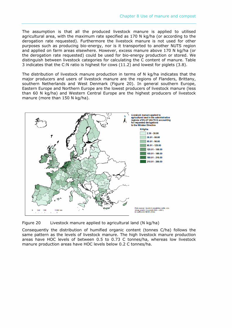
The assumption is that all the produced livestock manure is applied to utilised agricultural area, with the maximum rate specified as 170 N kg/ha (or according to the derogation rate requested). Furthermore the livestock manure is not used for other purposes such as producing bio-energy, nor is it transported to another NUTS region and applied on farm areas elsewhere. However, excess manure above 170 N kg/ha (or the derogation rate requested) could be used for bio-energy production or stored. We distinguish between livestock categories for calculating the C content of manure. Table 3 indicates that the C:N ratio is highest for cows (11.2) and lowest for piglets (3.8). The distribution of livestock manure production in terms of N kg/ha indicates that the major producers and users of livestock manure are the regions of Flanders, Brittany, southern Netherlands and West Denmark (Figure 20). In general southern Europe, Eastern Europe and Northern Europe are the lowest producers of livestock manure (less than 60 N kg/ha) and Western Central Europe are the highest producers of livestock manure (more than 150 N kg/ha).
Figure 20 Livestock manure applied to agricultural land (N kg/ha)
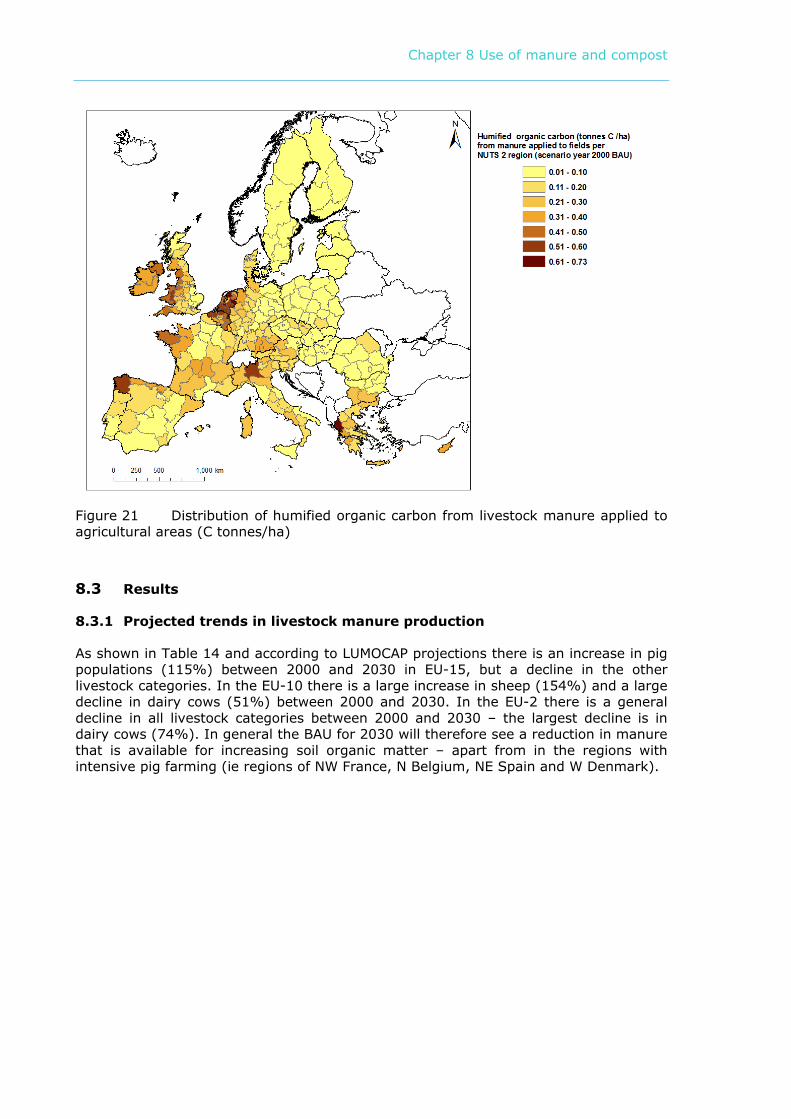
Consequently the distribution of humified organic content (tonnes C/ha) follows the same pattern as the levels of livestock manure. The high livestock manure production areas have HOC levels of between 0.5 to 0.73 C tonnes/ha, whereas low livestock manure production areas have HOC levels below 0.2 C tonnes/ha.
Chapter 8 Use of manure and compost
Figure 21 Distribution of humified organic carbon from livestock manure applied to agricultural areas (C tonnes/ha)
8.3 Results
8.3.1 Projected trends in livestock manure production
As shown in Table 14 and according to LUMOCAP projections there is an increase in pig populations (115%) between 2000 and 2030 in EU-15, but a decline in the other livestock categories. In the EU-10 there is a large increase in sheep (154%) and a large decline in dairy cows (51%) between 2000 and 2030. In the EU-2 there is a general decline in all livestock categories between 2000 and 2030 – the largest decline is in dairy cows (74%). In general the BAU for 2030 will therefore see a reduction in manure that is available for increasing soil organic matter – apart from in the regions with intensive pig farming (ie regions of NW France, N Belgium, NE Spain and W Denmark).
Chapter 8 Use of manure and compost
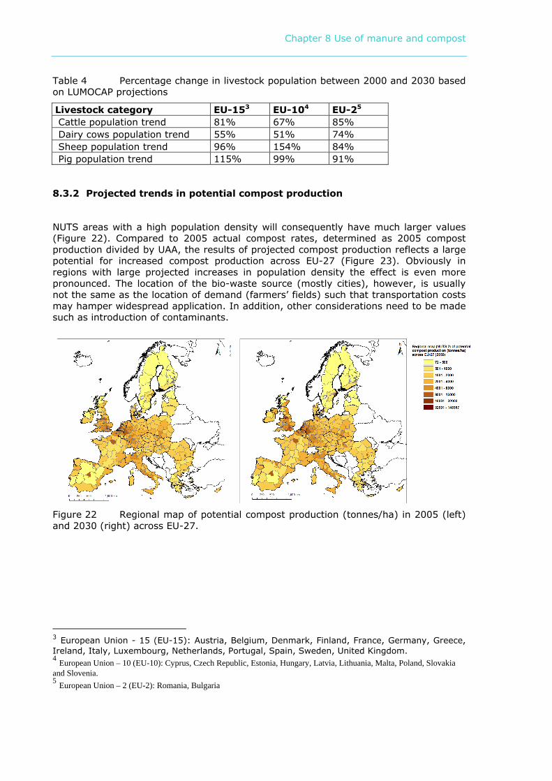
Table 4 Percentage change in livestock population between 2000 and 2030 based on LUMOCAP projections
Livestock category EU-153 EU-104 EU-25 Cattle population trend 81% 67% 85% Dairy cows population trend 55% 51% 74% Sheep population trend 96% 154% 84% Pig population trend 115% 99% 91% 8.3.2 Projected trends in potential compost production
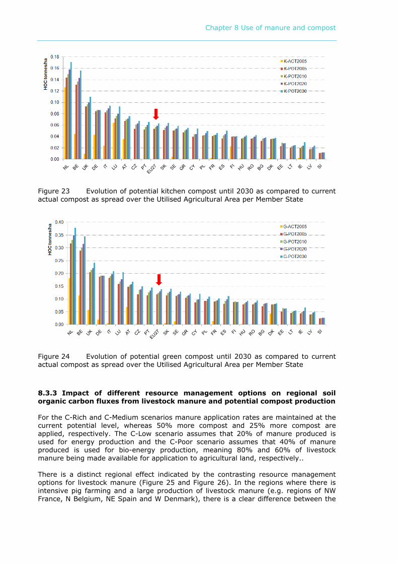
NUTS areas with a high population density will consequently have much larger values (Figure 22). Compared to 2005 actual compost rates, determined as 2005 compost production divided by UAA, the results of projected compost production reflects a large potential for increased compost production across EU-27 (Figure 23). Obviously in regions with large projected increases in population density the effect is even more pronounced. The location of the bio-waste source (mostly cities), however, is usually not the same as the location of demand (farmers’ fields) such that transportation costs may hamper widespread application. In addition, other considerations need to be made such as introduction of contaminants.
Figure 22 Regional map of potential compost production (tonnes/ha) in 2005 (left) and 2030 (right) across EU-27.
3 European Union - 15 (EU-15): Austria, Belgium, Denmark, Finland, France, Germany, Greece, Ireland, Italy, Luxembourg, Netherlands, Portugal, Spain, Sweden, United Kingdom. 4 European Union – 10 (EU-10): Cyprus, Czech Republic, Estonia, Hungary, Latvia, Lithuania, Malta, Poland, Slovakia and Slovenia. 5 European Union – 2 (EU-2): Romania, Bulgaria
Chapter 8 Use of manure and compost
Figure 23 Evolution of potential kitchen compost until 2030 as compared to current actual compost as spread over the Utilised Agricultural Area per Member State
Figure 24 Evolution of potential green compost until 2030 as compared to current actual compost as spread over the Utilised Agricultural Area per Member State
8.3.3 Impact of different resource management options on regional soil organic carbon fluxes from livestock manure and potential compost production
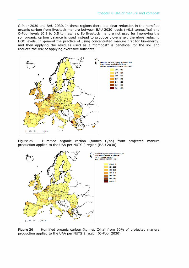
For the C-Rich and C-Medium scenarios manure application rates are maintained at the current potential level, whereas 50% more compost and 25% more compost are applied, respectively. The C-Low scenario assumes that 20% of manure produced is used for energy production and the C-Poor scenario assumes that 40% of manure produced is used for bio-energy production, meaning 80% and 60% of livestock manure being made available for application to agricultural land, respectively.. There is a distinct regional effect indicated by the contrasting resource management options for livestock manure (Figure 25 and Figure 26). In the regions where there is intensive pig farming and a large production of livestock manure (e.g. regions of NW France, N Belgium, NE Spain and W Denmark), there is a clear difference between the
Chapter 8 Use of manure and compost
C-Poor 2030 and BAU 2030. In these regions there is a clear reduction in the humified organic carbon from livestock manure between BAU 2030 levels (>0.5 tonnes/ha) and C-Poor levels (0.3 to 0.5 tonnes/ha). So livestock manure not used for improving the soil organic carbon balance is used instead to produce bio-energy, therefore reducing HOC levels. In general the practice of using concentrated manure first for bio-energy, and then applying the residues used as a “compost” is beneficial for the soil and reduces the risk of applying excessive nutrients.
Figure 25 Humified organic carbon (tonnes C/ha) from projected manure production applied to the UAA per NUTS 2 region (BAU 2030)
Figure 26 Humified organic carbon (tonnes C/ha) from 60% of projected manure production applied to the UAA per NUTS 2 region (C-Poor 2030)
Chapter 8 Use of manure and compost
8.3.4 Lifestock manure
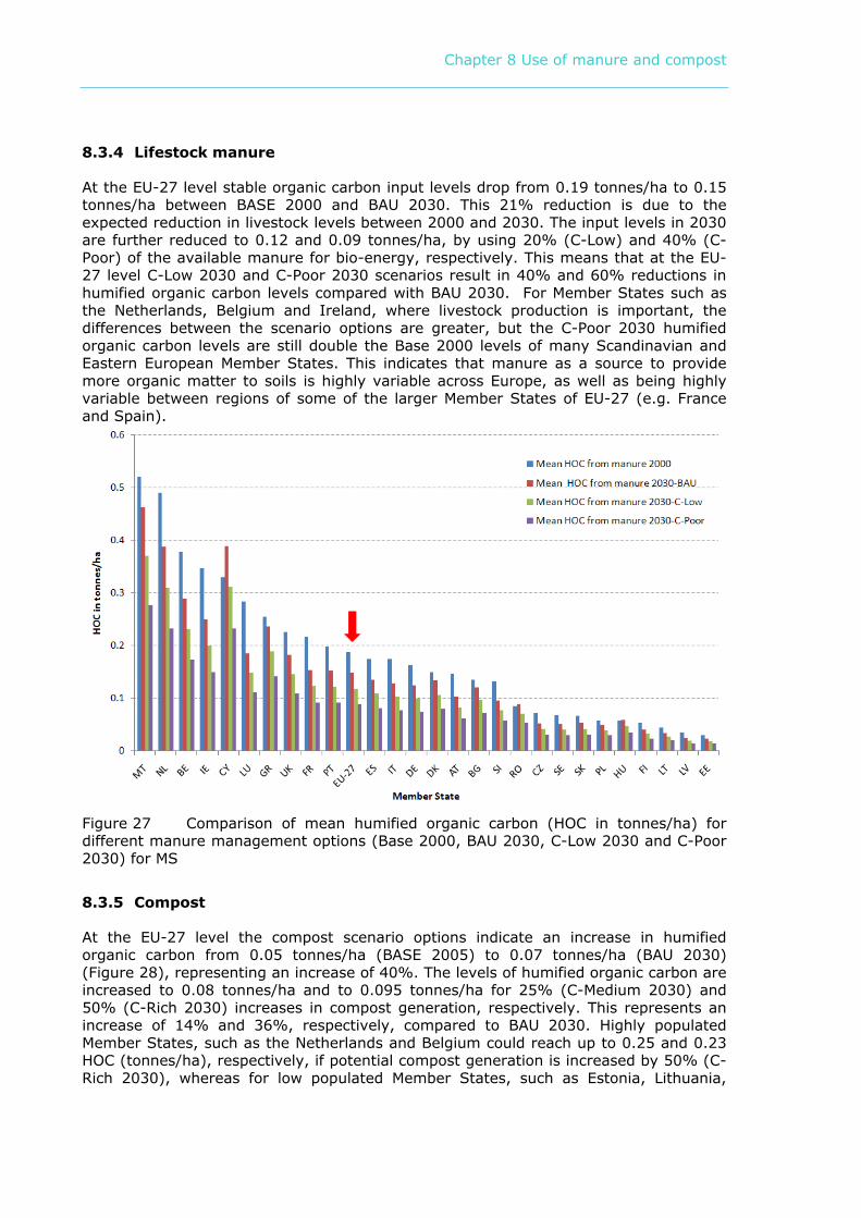
At the EU-27 level stable organic carbon input levels drop from 0.19 tonnes/ha to 0.15 tonnes/ha between BASE 2000 and BAU 2030. This 21% reduction is due to the expected reduction in livestock levels between 2000 and 2030. The input levels in 2030 are further reduced to 0.12 and 0.09 tonnes/ha, by using 20% (C-Low) and 40% (C-Poor) of the available manure for bio-energy, respectively. This means that at the EU-27 level C-Low 2030 and C-Poor 2030 scenarios result in 40% and 60% reductions in humified organic carbon levels compared with BAU 2030. For Member States such as the Netherlands, Belgium and Ireland, where livestock production is important, the differences between the scenario options are greater, but the C-Poor 2030 humified organic carbon levels are still double the Base 2000 levels of many Scandinavian and Eastern European Member States. This indicates that manure as a source to provide more organic matter to soils is highly variable across Europe, as well as being highly variable between regions of some of the larger Member States of EU-27 (e.g. France and Spain).
Figure 27 Comparison of mean humified organic carbon (HOC in tonnes/ha) for different manure management options (Base 2000, BAU 2030, C-Low 2030 and C-Poor 2030) for MS
8.3.5 Compost
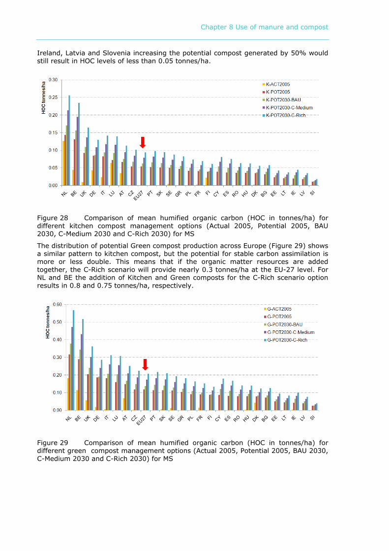
At the EU-27 level the compost scenario options indicate an increase in humified organic carbon from 0.05 tonnes/ha (BASE 2005) to 0.07 tonnes/ha (BAU 2030) (Figure 28), representing an increase of 40%. The levels of humified organic carbon are increased to 0.08 tonnes/ha and to 0.095 tonnes/ha for 25% (C-Medium 2030) and 50% (C-Rich 2030) increases in compost generation, respectively. This represents an increase of 14% and 36%, respectively, compared to BAU 2030. Highly populated Member States, such as the Netherlands and Belgium could reach up to 0.25 and 0.23 HOC (tonnes/ha), respectively, if potential compost generation is increased by 50% (C-Rich 2030), whereas for low populated Member States, such as Estonia, Lithuania,
Chapter 8 Use of manure and compost
Ireland, Latvia and Slovenia increasing the potential compost generated by 50% would still result in HOC levels of less than 0.05 tonnes/ha.
Figure 28 Comparison of mean humified organic carbon (HOC in tonnes/ha) for different kitchen compost management options (Actual 2005, Potential 2005, BAU 2030, C-Medium 2030 and C-Rich 2030) for MS
The distribution of potential Green compost production across Europe (Figure 29) shows a similar pattern to kitchen compost, but the potential for stable carbon assimilation is more or less double. This means that if the organic matter resources are added together, the C-Rich scenario will provide nearly 0.3 tonnes/ha at the EU-27 level. For NL and BE the addition of Kitchen and Green composts for the C-Rich scenario option results in 0.8 and 0.75 tonnes/ha, respectively.
Figure 29 Comparison of mean humified organic carbon (HOC in tonnes/ha) for different green compost management options (Actual 2005, Potential 2005, BAU 2030, C-Medium 2030 and C-Rich 2030) for MS

Chapter 8 Use of manure and compost
Chapter 9 Use of forest residues
CHAPTER 9 USE OF FOREST RESIDUES
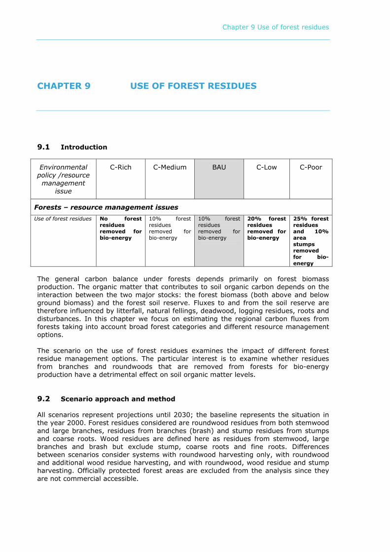
9.1 Introduction
Environmental policy /resource management
issue
C-Rich C-Medium BAU C-Low C-Poor
Forests – resource management issues
Use of forest residues No forest residues removed for bio-energy
10% forest residues removed for bio-energy
10% forest residues removed for bio-energy
20% forest residues removed for bio-energy
25% forest residues and 10% area stumps removed for bio-energy
The general carbon balance under forests depends primarily on forest biomass production. The organic matter that contributes to soil organic carbon depends on the interaction between the two major stocks: the forest biomass (both above and below ground biomass) and the forest soil reserve. Fluxes to and from the soil reserve are therefore influenced by litterfall, natural fellings, deadwood, logging residues, roots and disturbances. In this chapter we focus on estimating the regional carbon fluxes from forests taking into account broad forest categories and different resource management options. The scenario on the use of forest residues examines the impact of different forest residue management options. The particular interest is to examine whether residues from branches and roundwoods that are removed from forests for bio-energy production have a detrimental effect on soil organic matter levels.
9.2 Scenario approach and method
All scenarios represent projections until 2030; the baseline represents the situation in the year 2000. Forest residues considered are roundwood residues from both stemwood and large branches, residues from branches (brash) and stump residues from stumps and coarse roots. Wood residues are defined here as residues from stemwood, large branches and brash but exclude stump, coarse roots and fine roots. Differences between scenarios consider systems with roundwood harvesting only, with roundwood and additional wood residue harvesting, and with roundwood, wood residue and stump harvesting. Officially protected forest areas are excluded from the analysis since they are not commercial accessible.
Chapter 9 Use of forest residues
In the C-Rich 2030 scenario, all forest residues are left on-site. In C-Medium and BAU 2030 10% of forest residue from branches and roundwood is removed for bio-energy purposes in addition to regular roundwood removal. In C-Low 2030 scenario this removal amounts to 20% and in the C-Poor 2030 scenario 25 % of forest brash is being removed in addition to the removal of stumps which is assumed to occur on 10% of the forest surface area. A maximum residue removal scenario (or Worst Case 2030) is also considered since the use of brash and, to a lesser extent, of stumps is rapidly increasing. Despite the poor understanding of the impacts of stump removal and collecting of logging residue on the nutrient cycle, microbiology, restocking, carbon balance, and succession of vegetation, current certification schemes (FSC and PEFC) require that a certain share of biomass must be left on the forest floor for soil protection and biodiversity purposes. In the maximum residue removal scenario (or Worst Case 2030), we assume 70% wood residue removal and 25% stump removal. The analysis assumes that in all scenarios foliage (needles and leaves) is left on the forest floor and is not available for energy use but decays faster in the case of stump removal, because stump removal exposes foliage to more rainfall and temperature changes. The following scenarios are carried out for both coniferous and broadleaved forests:
1. Baseline year 2000 – 0% residues harvested 2. Baseline, C-Rich: year 2030 - 0% residues harvested 3. C-Medium and BAU: year 2030 – 10% residues harvested 4. C-Low: year 2030 - 20% residues harvested 5. C-Poor: year 2030 - 25% residues harvested plus 10% stumps removal 6. Worst case: year 2030 - 70% residues harvested plus 25% stump removal
The following steps are taken in the analysis:
1. UNECE/TBFRA data are used to estimate the total above and below-ground biomass for broadleaved and coniferous forests for the baseline 2000 and 2030; 2. REGSOM uses allometric parameters to determine the above-ground biomass, the below-ground biomass and the litterfall. Different turn-over and humification functions are subsequently included to derive the flux of humified organic carbon (HOC) to the forest soil per hectare; and, 3. REGSOM derives humified organic carbon (HOC) maps (tonnes/ha) for each of the specified scenarios to compare the impact of different resource management options on regional soil organic carbon fluxes from forest residues.
9.3 Production of organic matter from forests
9.3.1 Forest biomass production
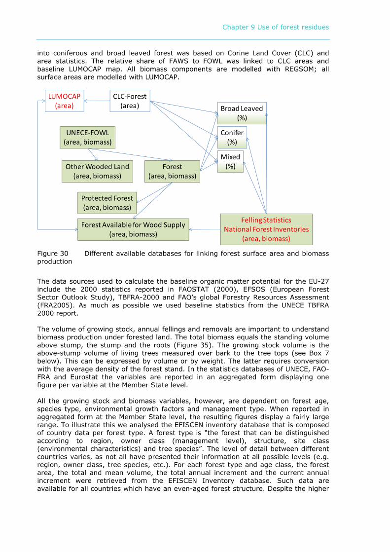
In order to link biomass production to forest surface area, several databases had to be connected. Land use/cover maps represent data closer to forest and other wood land (FOWL) (Figure 30), whereas inventories and statistics relate to forest area available for wood supply (FAWS) provide information on stocks and potential management practices. For biomass production we relied on national felling statistics and inventories which ultimately enable determining the different components of the forest soil organic carbon balance. Subsequently, the biomass production had to be coupled to the LUMOCAP land cover map. Time series of felling statistics and national inventories mostly apply to forests available for wood supply (FAWS) as the growing stock of these type of forests are monitored closely. The TBFRA (UNECE, 2000), however, reported on forest and other wood land (FOWL) areas, protected forest and other wood land (OWL) areas and the share of FAWS to FOWL for the year 2000. We linked these to the LUMOCAP 2000 baseline map which only includes the class ‘forest’. Areal distribution
Chapter 9 Use of forest residues
into coniferous and broad leaved forest was based on Corine Land Cover (CLC) and area statistics. The relative share of FAWS to FOWL was linked to CLC areas and baseline LUMOCAP map. All biomass components are modelled with REGSOM; all surface areas are modelled with LUMOCAP.
UNECE-FOWL(area, biomass)
LUMOCAP(area)
Protected Forest(area, biomass)
Forest(area, biomass)
Other Wooded Land(area, biomass)
Forest Available for Wood Supply(area, biomass)
Felling StatisticsNational Forest Inventories
(area, biomass)
Conifer(%)
Broad Leaved(%)
Mixed(%)
CLC-Forest(area)
Figure 30 Different available databases for linking forest surface area and biomass production
The data sources used to calculate the baseline organic matter potential for the EU-27 include the 2000 statistics reported in FAOSTAT (2000), EFSOS (European Forest Sector Outlook Study), TBFRA-2000 and FAO’s global Forestry Resources Assessment (FRA2005). As much as possible we used baseline statistics from the UNECE TBFRA 2000 report. The volume of growing stock, annual fellings and removals are important to understand biomass production under forested land. The total biomass equals the standing volume above stump, the stump and the roots (Figure 35). The growing stock volume is the above-stump volume of living trees measured over bark to the tree tops (see Box 7 below). This can be expressed by volume or by weight. The latter requires conversion with the average density of the forest stand. In the statistics databases of UNECE, FAO-FRA and Eurostat the variables are reported in an aggregated form displaying one figure per variable at the Member State level. All the growing stock and biomass variables, however, are dependent on forest age, species type, environmental growth factors and management type. When reported in aggregated form at the Member State level, the resulting figures display a fairly large range. To illustrate this we analysed the EFISCEN inventory database that is composed of country data per forest type. A forest type is "the forest that can be distinguished according to region, owner class (management level), structure, site class (environmental characteristics) and tree species”. The level of detail between different countries varies, as not all have presented their information at all possible levels (e.g. region, owner class, tree species, etc.). For each forest type and age class, the forest area, the total and mean volume, the total annual increment and the current annual increment were retrieved from the EFISCEN Inventory database. Such data are available for all countries which have an even-aged forest structure. Despite the higher
Chapter 9 Use of forest residues
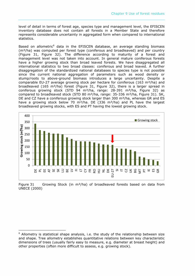
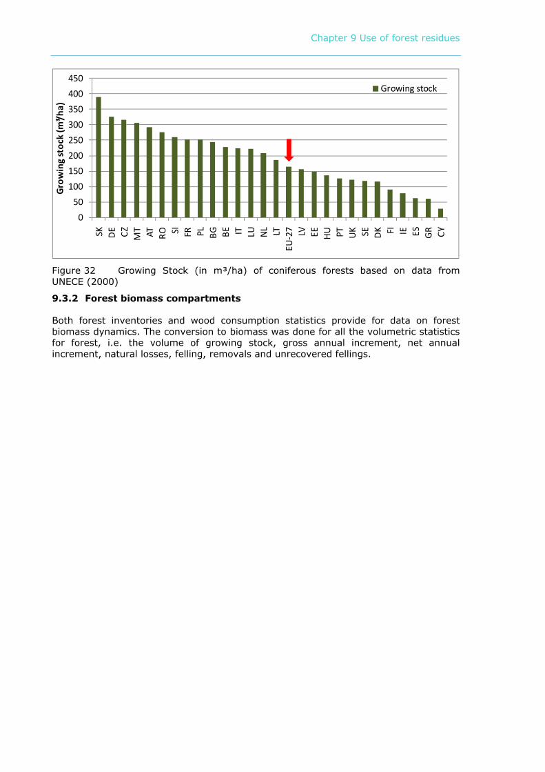
level of detail in terms of forest age, species type and management level, the EFISCEN inventory database does not contain all forests in a Member State and therefore represents considerable uncertainty in aggregated form when compared to international statistics. Based on allometric6 data in the EFISCEN database, an average standing biomass (m³/ha) was computed per forest type (coniferous and broadleaved) and per country (Figure 31, Figure 32). The difference according to maturity of a forest and management level was not taken into account. In general mature coniferous forests have a higher growing stock than broad leaved forests. We have disaggregated all international statistics to two broad classes: coniferous and broad leaved. A further disaggregation of the standardized national databases to species type is not possible since the current national aggregation of parameters such as wood density or stump/roots to above-ground biomass introduces a large uncertainty. Despite a comparable EU-27 average growing stock per hectare for coniferous (163 m³/ha) and broadleaved (165 m³/ha) forest (Figure 31, Figure 32), there is a larger spread in coniferous growing stock (STD 94 m³/ha, range: 28-391 m³/ha, Figure 32) as compared to broadleaved stock (STD 80 m³/ha, range: 35-336 m³/ha, Figure 31). SK, DE and CZ have a coniferous growing stock larger than 300 m³/ha, whereas GR and ES have a growing stock below 70 m³/ha. DE (336 m³/ha) and PL have the largest broadleaved growing stocks, with ES and PT having the lowest growing stock.
0
50
100
150
200
250
300
350
400
DE PL EE AT SE SK LU BE LV FI LT CY FR RO HU NL
DK
EU-2
7 SI IT CZ UK
BG MT PT IE ES GR
Gro
win
g st
ock
(m³/h
a)
Growing stock
Figure 31 Growing Stock (in m³/ha) of broadleaved forests based on data from UNECE (2000)
6 Allometry is statistical shape analysis, i.e. the study of the relationship between size and shape. Tree allometry establishes quantitative relations between key characteristic dimensions of trees (usually fairly easy to measure, e.g. diameter at breast height) and other properties (often more difficult to assess, e.g. growing stock).
Chapter 9 Use of forest residues
0
50
100
150
200
250
300
350
400
450
SK DE CZ MT AT RO SI FR PL BG BE IT LU NL LT
EU-2
7 LV EE HU PT UK SE DK FI IE ES GR CY
Gro
win
g st
ock
(m³/h
a)
Growing stock
Figure 32 Growing Stock (in m³/ha) of coniferous forests based on data from UNECE (2000)
9.3.2 Forest biomass compartments
Both forest inventories and wood consumption statistics provide for data on forest biomass dynamics. The conversion to biomass was done for all the volumetric statistics for forest, i.e. the volume of growing stock, gross annual increment, net annual increment, natural losses, felling, removals and unrecovered fellings.
Chapter 9 Use of forest residues
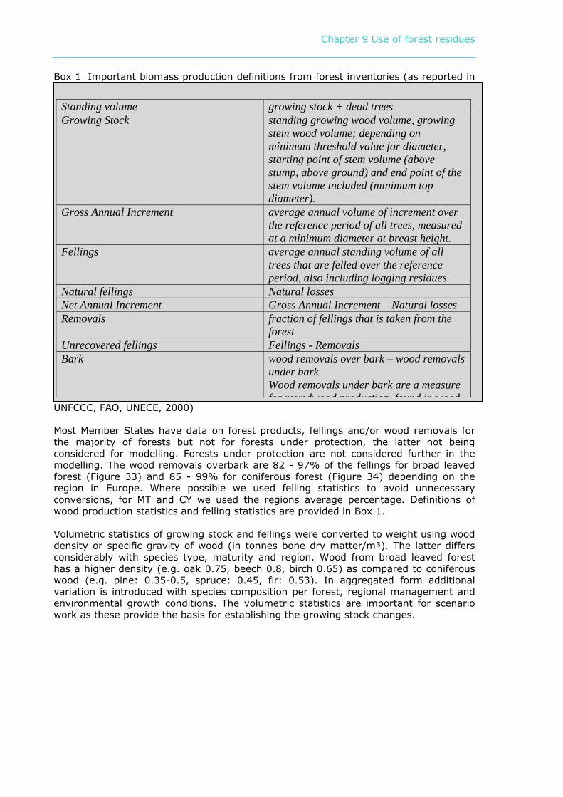
Box 1 Important biomass production definitions from forest inventories (as reported in
UNFCCC, FAO, UNECE, 2000) Most Member States have data on forest products, fellings and/or wood removals for the majority of forests but not for forests under protection, the latter not being considered for modelling. Forests under protection are not considered further in the modelling. The wood removals overbark are 82 - 97% of the fellings for broad leaved forest (Figure 33) and 85 - 99% for coniferous forest (Figure 34) depending on the region in Europe. Where possible we used felling statistics to avoid unnecessary conversions, for MT and CY we used the regions average percentage. Definitions of wood production statistics and felling statistics are provided in Box 1. Volumetric statistics of growing stock and fellings were converted to weight using wood density or specific gravity of wood (in tonnes bone dry matter/m³). The latter differs considerably with species type, maturity and region. Wood from broad leaved forest has a higher density (e.g. oak 0.75, beech 0.8, birch 0.65) as compared to coniferous wood (e.g. pine: 0.35-0.5, spruce: 0.45, fir: 0.53). In aggregated form additional variation is introduced with species composition per forest, regional management and environmental growth conditions. The volumetric statistics are important for scenario work as these provide the basis for establishing the growing stock changes.
Standing volume growing stock + dead trees Growing Stock standing growing wood volume, growing
stem wood volume; depending on minimum threshold value for diameter, starting point of stem volume (above stump, above ground) and end point of the stem volume included (minimum top diameter).
Gross Annual Increment average annual volume of increment over the reference period of all trees, measured at a minimum diameter at breast height.
Fellings average annual standing volume of all trees that are felled over the reference period, also including logging residues.
Natural fellings Natural losses Net Annual Increment Gross Annual Increment – Natural losses Removals fraction of fellings that is taken from the
forest Unrecovered fellings Fellings - Removals Bark wood removals over bark – wood removals
under bark Wood removals under bark are a measure for roundwood production found in wood
Chapter 9 Use of forest residues
0123456789
10
EE PL FI SE AT DK SK LV DE
NL
HU LT BE CY LU FR
EU-2
7 PT RO CZ BG GR
MT
UK SI ES IT IE
Volu
me
(m³/h
a)
Felling
Removal
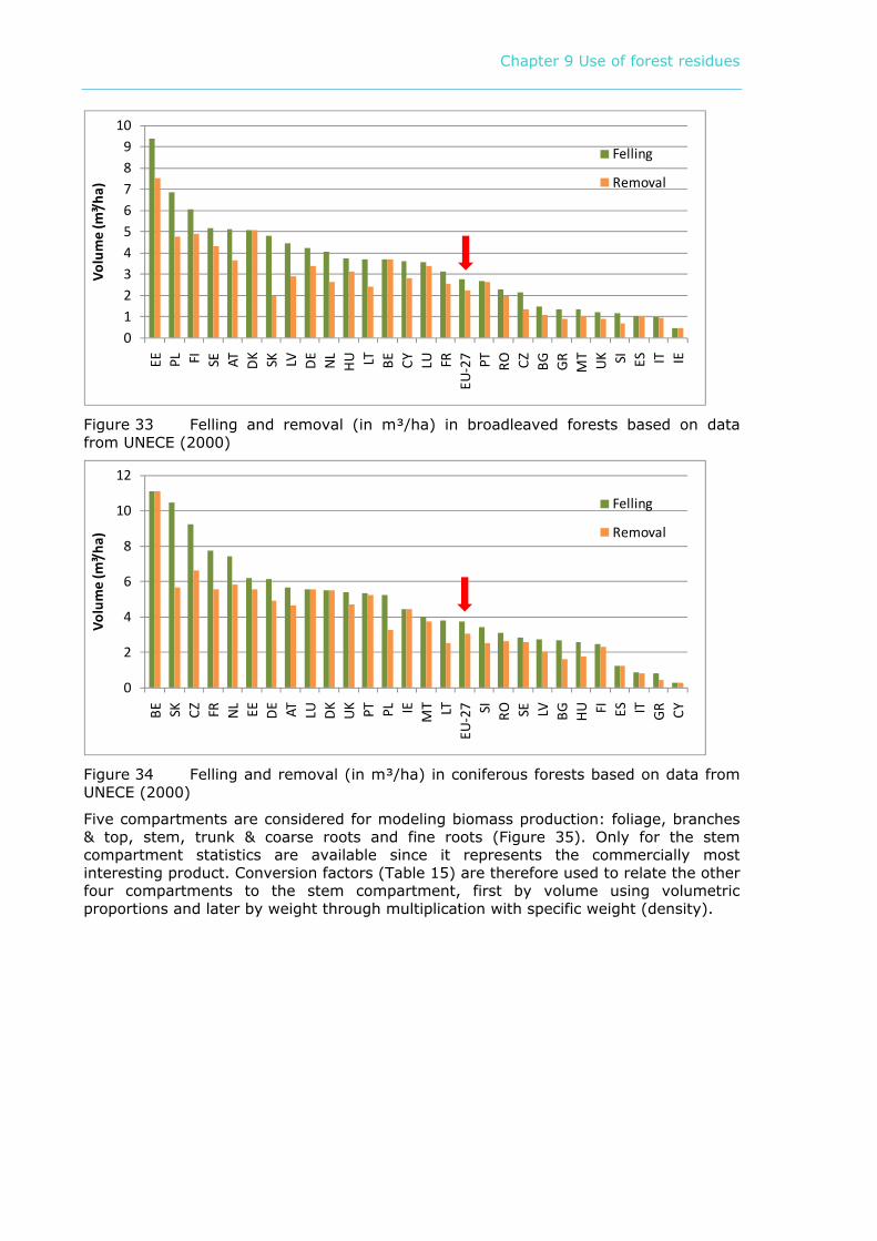
Figure 33 Felling and removal (in m³/ha) in broadleaved forests based on data from UNECE (2000)
0
2
4
6
8
10
12
BE SK CZ FR NL EE DE AT LU DK
UK PT PL IE
MT LT
EU-2
7 SI RO SE LV BG HU FI ES IT GR CY
Volu
me
(m³/h
a)
Felling
Removal
Figure 34 Felling and removal (in m³/ha) in coniferous forests based on data from UNECE (2000)
Five compartments are considered for modeling biomass production: foliage, branches & top, stem, trunk & coarse roots and fine roots (Figure 35). Only for the stem compartment statistics are available since it represents the commercially most interesting product. Conversion factors (Table 15) are therefore used to relate the other four compartments to the stem compartment, first by volume using volumetric proportions and later by weight through multiplication with specific weight (density).
Chapter 9 Use of forest residues
Stem
TopØ > 7 cm
Trunk
Fineroots
Twigs
Branches
Branches Top Foliage (leaves or needles)
LitterfallLitterfall
AB
C
D
E
F
GH
C
AB
D
E HF
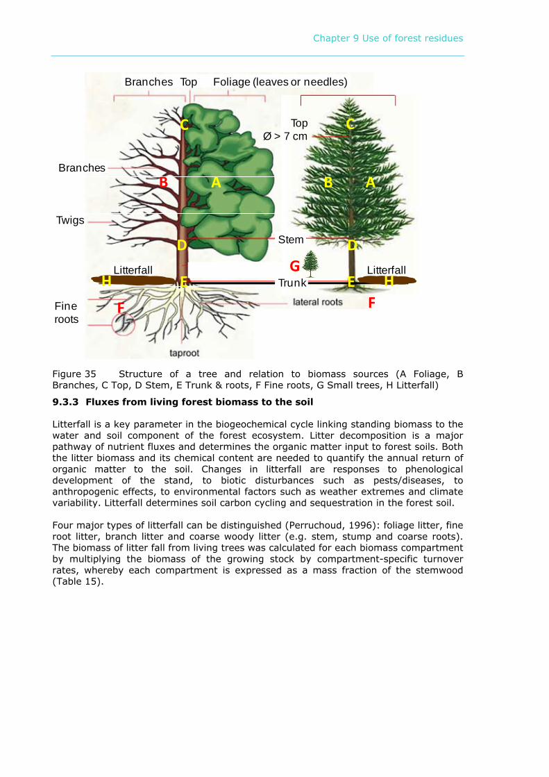
Figure 35 Structure of a tree and relation to biomass sources (A Foliage, B Branches, C Top, D Stem, E Trunk & roots, F Fine roots, G Small trees, H Litterfall)
9.3.3 Fluxes from living forest biomass to the soil
Litterfall is a key parameter in the biogeochemical cycle linking standing biomass to the water and soil component of the forest ecosystem. Litter decomposition is a major pathway of nutrient fluxes and determines the organic matter input to forest soils. Both the litter biomass and its chemical content are needed to quantify the annual return of organic matter to the soil. Changes in litterfall are responses to phenological development of the stand, to biotic disturbances such as pests/diseases, to anthropogenic effects, to environmental factors such as weather extremes and climate variability. Litterfall determines soil carbon cycling and sequestration in the forest soil. Four major types of litterfall can be distinguished (Perruchoud, 1996): foliage litter, fine root litter, branch litter and coarse woody litter (e.g. stem, stump and coarse roots). The biomass of litter fall from living trees was calculated for each biomass compartment by multiplying the biomass of the growing stock by compartment-specific turnover rates, whereby each compartment is expressed as a mass fraction of the stemwood (Table 15).
Chapter 9 Use of forest residues
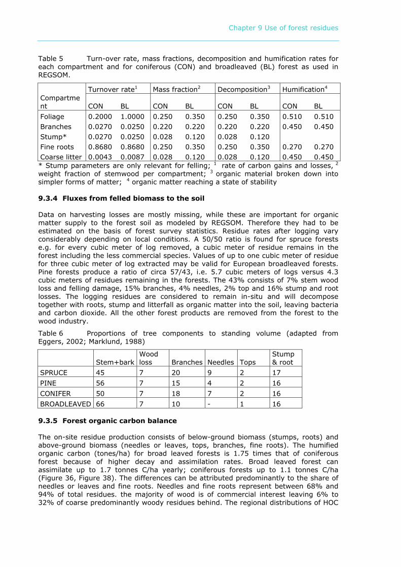
Table 5 Turn-over rate, mass fractions, decomposition and humification rates for each compartment and for coniferous (CON) and broadleaved (BL) forest as used in REGSOM.
Turnover rate1 Mass fraction2 Decomposition3 Humification4 Compartment CON BL CON BL CON BL CON BL Foliage 0.2000 1.0000 0.250 0.350 0.250 0.350 0.510 0.510 Branches 0.0270 0.0250 0.220 0.220 0.220 0.220 0.450 0.450 Stump* 0.0270 0.0250 0.028 0.120 0.028 0.120 Fine roots 0.8680 0.8680 0.250 0.350 0.250 0.350 0.270 0.270 Coarse litter 0.0043 0.0087 0.028 0.120 0.028 0.120 0.450 0.450 * Stump parameters are only relevant for felling; 1 rate of carbon gains and losses, 2 weight fraction of stemwood per compartment; 3 organic material broken down into simpler forms of matter; 4 organic matter reaching a state of stability 9.3.4 Fluxes from felled biomass to the soil
Data on harvesting losses are mostly missing, while these are important for organic matter supply to the forest soil as modeled by REGSOM. Therefore they had to be estimated on the basis of forest survey statistics. Residue rates after logging vary considerably depending on local conditions. A 50/50 ratio is found for spruce forests e.g. for every cubic meter of log removed, a cubic meter of residue remains in the forest including the less commercial species. Values of up to one cubic meter of residue for three cubic meter of log extracted may be valid for European broadleaved forests. Pine forests produce a ratio of circa 57/43, i.e. 5.7 cubic meters of logs versus 4.3 cubic meters of residues remaining in the forests. The 43% consists of 7% stem wood loss and felling damage, 15% branches, 4% needles, 2% top and 16% stump and root losses. The logging residues are considered to remain in-situ and will decompose together with roots, stump and litterfall as organic matter into the soil, leaving bacteria and carbon dioxide. All the other forest products are removed from the forest to the wood industry.
Table 6 Proportions of tree components to standing volume (adapted from Eggers, 2002; Marklund, 1988)
Stem+bark Wood loss Branches Needles Tops
Stump & root
SPRUCE 45 7 20 9 2 17 PINE 56 7 15 4 2 16 CONIFER 50 7 18 7 2 16 BROADLEAVED 66 7 10 - 1 16 9.3.5 Forest organic carbon balance
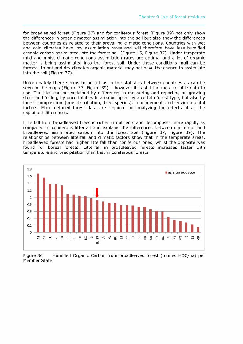
The on-site residue production consists of below-ground biomass (stumps, roots) and above-ground biomass (needles or leaves, tops, branches, fine roots). The humified organic carbon (tones/ha) for broad leaved forests is 1.75 times that of coniferous forest because of higher decay and assimilation rates. Broad leaved forest can assimilate up to 1.7 tonnes C/ha yearly; coniferous forests up to 1.1 tonnes C/ha (Figure 36, Figure 38). The differences can be attributed predominantly to the share of needles or leaves and fine roots. Needles and fine roots represent between 68% and 94% of total residues. the majority of wood is of commercial interest leaving 6% to 32% of coarse predominantly woody residues behind. The regional distributions of HOC
Chapter 9 Use of forest residues
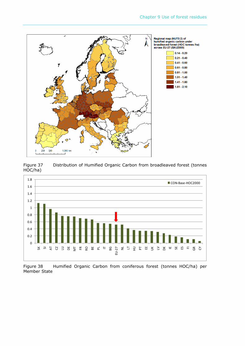
for broadleaved forest (Figure 37) and for coniferous forest (Figure 39) not only show the differences in organic matter assimilation into the soil but also show the differences between countries as related to their prevailing climatic conditions. Countries with wet and cold climates have low assimilation rates and will therefore have less humified organic carbon assimilated into the forest soil (Figure 15, Figure 37). Under temperate mild and moist climatic conditions assimilation rates are optimal and a lot of organic matter is being assimilated into the forest soil. Under these conditions mull can be formed. In hot and dry climates organic material may not have the chance to assimilate into the soil (Figure 37). Unfortunately there seems to be a bias in the statistics between countries as can be seen in the maps (Figure 37, Figure 39) – however it is still the most reliable data to use. The bias can be explained by differences in measuring and reporting on growing stock and felling, by uncertainties in area occupied by a certain forest type, but also by forest composition (age distribution, tree species), management and environmental factors. More detailed forest data are required for analyzing the effects of all the explained differences. Litterfall from broadleaved trees is richer in nutrients and decomposes more rapidly as compared to coniferous litterfall and explains the differences between coniferous and broadleaved assimilated carbon into the forest soil (Figure 37, Figure 39). The relationships between litterfall and climatic factors show that in the temperate areas, broadleaved forests had higher litterfall than coniferous ones, whilst the opposite was found for boreal forests. Litterfall in broadleaved forests increases faster with temperature and precipitation than that in coniferous forests.
0
0.2
0.4
0.6
0.8
1
1.2
1.4
1.6
1.8
AT
DE
LU PL SK BE EE FR RO SI
EU-2
7 LV NL
HU LT CZ IT SE DK
UK CY BG FI PT MT IE ES GR
BL-BASE-HOC2000
Figure 36 Humified Organic Carbon from broadleaved forest (tonnes HOC/ha) per Member State
Chapter 9 Use of forest residues
Figure 37 Distribution of Humified Organic Carbon from broadleaved forest (tonnes HOC/ha)
0
0.2
0.4
0.6
0.8
1
1.2
1.4
1.6
1.8
SK SI AT
CZ LU DE
MT FR RO BE PL IT BG
EU-2
7 NL LT HU PT EE UK LV DK IE SE ES FI GR CY
CON-Base-HOC2000
Figure 38 Humified Organic Carbon from coniferous forest (tonnes HOC/ha) per Member State
Chapter 9 Use of forest residues
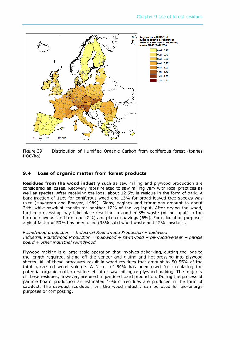
Figure 39 Distribution of Humified Organic Carbon from coniferous forest (tonnes HOC/ha)
9.4 Loss of organic matter from forest products
Residues from the wood industry such as saw milling and plywood production are considered as losses. Recovery rates related to saw milling vary with local practices as well as species. After receiving the logs, about 12.5% is residue in the form of bark. A bark fraction of 11% for coniferous wood and 13% for broad-leaved tree species was used (Haygreen and Bowyer, 1989). Slabs, edgings and trimmings amount to about 34% while sawdust constitutes another 12% of the log input. After drying the wood, further processing may take place resulting in another 8% waste (of log input) in the form of sawdust and trim end (2%) and planer shavings (6%). For calculation purposes a yield factor of 50% has been used (38% solid wood waste and 12% sawdust). Roundwood production = Industrial Roundwood Production + fuelwood Industrial Roundwood Production = pulpwood + sawnwood + plywood/veneer + paricle board + other industrial roundwood Plywood making is a large-scale operation that involves debarking, cutting the logs to the length required, slicing off the veneer and gluing and hot-pressing into plywood sheets. All of these processes result in wood residues that amount to 50-55% of the total harvested wood volume. A factor of 50% has been used for calculating the potential organic matter residue left after saw milling or plywood making. The majority of these residues, however, are used in particle board production. During the process of particle board production an estimated 10% of residues are produced in the form of sawdust. The sawdust residues from the wood industry can be used for bio-energy purposes or composting.
Chapter 9 Use of forest residues
The off-site organic matter production consists of bark and wood waste. Countries with an important wood industry such as FI, SE, DE and FR obviously produce most of the off-site dry matter. These values may represent the amount of wood waste that could be used for bio-energy purposes, thereby displacing the need for harvesting felling residues that are valuable to building up soil organic matter. Estimated losses of organic matter from the wood industry should be used as the prime source for bio-energy purposes rather than harvesting logging residues and disturbing forest ecosystems.
9.5 Results
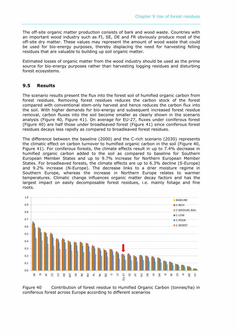
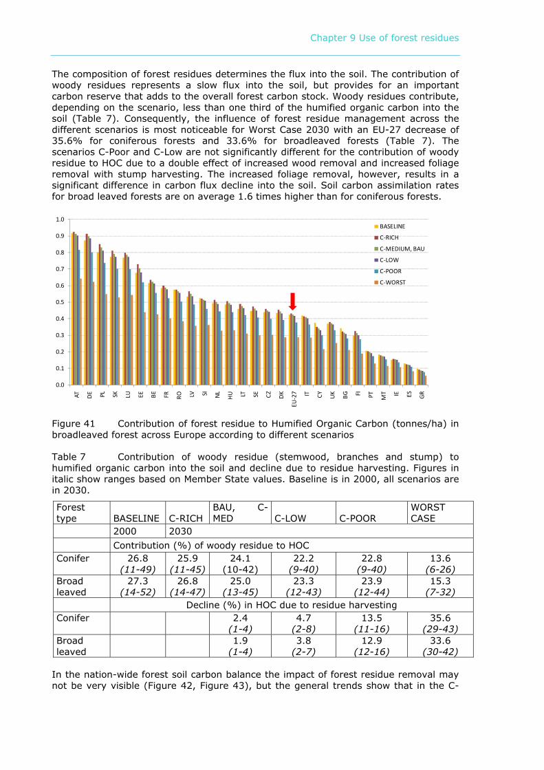
The scenario results present the flux into the forest soil of humified organic carbon from forest residues. Removing forest residues reduces the carbon stock of the forest compared with conventional stem-only harvest and hence reduces the carbon flux into the soil. With higher demands for bio-energy and subsequent increased forest residue removal, carbon fluxes into the soil become smaller as clearly shown in the scenario analysis (Figure 40, Figure 41). On average for EU-27, fluxes under coniferous forest (Figure 40) are half those under broadleaved forest (Figure 41) since coniferous forest residues decays less rapidly as compared to broadleaved forest residues. The difference between the baseline (2000) and the C-rich scenario (2030) represents the climatic effect on carbon turnover to humified organic carbon in the soil (Figure 40, Figure 41). For coniferous forests, the climate effects result in up to 7.4% decrease in humified organic carbon added to the soil as compared to baseline for Southern European Member States and up to 9.7% increase for Northern European Member States. For broadleaved forests, the climate effects are up to 6.3% decline (S-Europe) and 9.2% increase (N-Europe). The decrease links to a drier moisture regime in Southern Europe, whereas the increase in Northern Europe relates to warmer temperatures. Climatic change influences organic matter decay factors and has the largest impact on easily decomposable forest residues, i.e. mainly foliage and fine roots.
0.0
0.1
0.2
0.3
0.4
0.5
0.6
0.7
0.8
0.9
1.0
SK SI AT CZ LU DE
MT FR BE RO PL NL
BG IT LT
EU-2
7 EE PT HU UK LV DK IE SE ES FI GR CY
BASELINE
C-RICH
C-MEDIUM, BAU
C-LOW
C-POOR
C-WORST
Figure 40 Contribution of forest residue to Humified Organic Carbon (tonnes/ha) in coniferous forest across Europe according to different scenarios
Chapter 9 Use of forest residues
The composition of forest residues determines the flux into the soil. The contribution of woody residues represents a slow flux into the soil, but provides for an important carbon reserve that adds to the overall forest carbon stock. Woody residues contribute, depending on the scenario, less than one third of the humified organic carbon into the soil (Table 7). Consequently, the influence of forest residue management across the different scenarios is most noticeable for Worst Case 2030 with an EU-27 decrease of 35.6% for coniferous forests and 33.6% for broadleaved forests (Table 7). The scenarios C-Poor and C-Low are not significantly different for the contribution of woody residue to HOC due to a double effect of increased wood removal and increased foliage removal with stump harvesting. The increased foliage removal, however, results in a significant difference in carbon flux decline into the soil. Soil carbon assimilation rates for broad leaved forests are on average 1.6 times higher than for coniferous forests.
0.0
0.1
0.2
0.3
0.4
0.5
0.6
0.7
0.8
0.9
1.0
AT DE PL SK LU EE BE FR RO LV SI NL
HU LT SE CZ DK
EU-2
7 IT CY UK
BG FI PT MT IE ES GR
BASELINE
C-RICH
C-MEDIUM, BAU
C-LOW
C-POOR
C-WORST
Figure 41 Contribution of forest residue to Humified Organic Carbon (tonnes/ha) in broadleaved forest across Europe according to different scenarios
Table 7 Contribution of woody residue (stemwood, branches and stump) to humified organic carbon into the soil and decline due to residue harvesting. Figures in italic show ranges based on Member State values. Baseline is in 2000, all scenarios are in 2030.
Forest type BASELINE C-RICH
BAU, C-MED C-LOW C-POOR
WORST CASE
2000 2030 Contribution (%) of woody residue to HOC Conifer
26.8 (11-49)
25.9 (11-45)
24.1 (10-42)
22.2 (9-40)
22.8 (9-40)
13.6 (6-26)
Broad leaved
27.3 (14-52)
26.8 (14-47)
25.0 (13-45)
23.3 (12-43)
23.9 (12-44)
15.3 (7-32)
Decline (%) in HOC due to residue harvesting Conifer 2.4
(1-4) 4.7
(2-8) 13.5
(11-16) 35.6
(29-43) Broad leaved 1.9
(1-4) 3.8
(2-7) 12.9
(12-16) 33.6
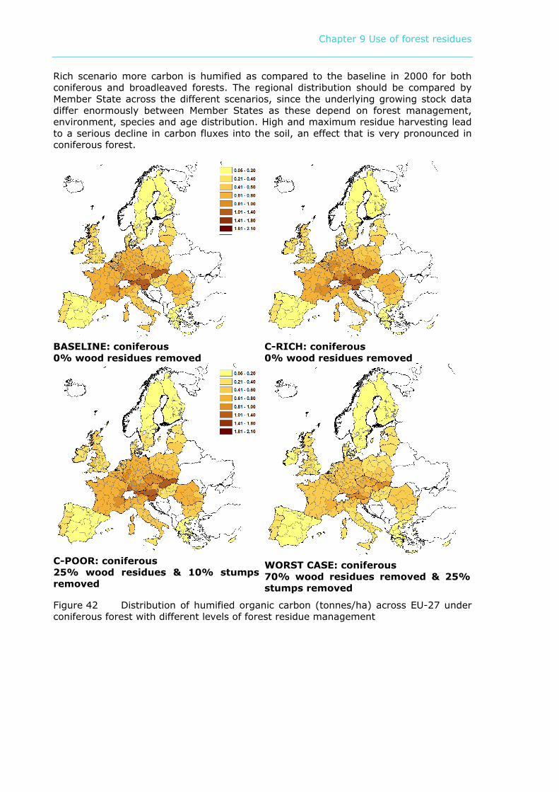
(30-42) In the nation-wide forest soil carbon balance the impact of forest residue removal may not be very visible (Figure 42, Figure 43), but the general trends show that in the C-
Chapter 9 Use of forest residues
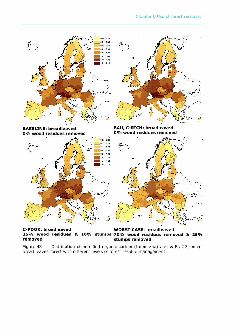
Rich scenario more carbon is humified as compared to the baseline in 2000 for both coniferous and broadleaved forests. The regional distribution should be compared by Member State across the different scenarios, since the underlying growing stock data differ enormously between Member States as these depend on forest management, environment, species and age distribution. High and maximum residue harvesting lead to a serious decline in carbon fluxes into the soil, an effect that is very pronounced in coniferous forest.
BASELINE: coniferous 0% wood residues removed
C-RICH: coniferous 0% wood residues removed
C-POOR: coniferous 25% wood residues & 10% stumps removed
WORST CASE: coniferous 70% wood residues removed & 25% stumps removed
Figure 42 Distribution of humified organic carbon (tonnes/ha) across EU-27 under coniferous forest with different levels of forest residue management
Chapter 9 Use of forest residues
BASELINE: broadleaved 0% wood residues removed
BAU, C-RICH: broadleaved 0% wood residues removed
C-POOR: broadleaved 25% wood residues & 10% stumps removed
WORST CASE: broadleaved 70% wood residues removed & 25% stumps removed
Figure 43 Distribution of humified organic carbon (tonnes/ha) across EU-27 under broad leaved forest with different levels of forest residue management
Chapter 10 Conservation of peatlands
CHAPTER 10 CONSERVATION OF PEATLANDS
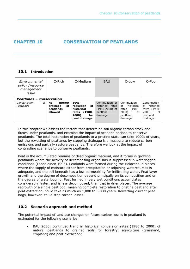
10.1 Introduction
Environmental policy /resource management
issue
C-Rich C-Medium BAU C-Low C-Poor
Peatlands – conservation Conservation of Peatlands
No further drainage of peatlands allowed
50% reduction of historical rates (1980-2000) for peat drainage
Continuation of historical rates (1980-2000) of peatland drainage
Continuation of historical rates (1980-2000) of peatland drainage
Continuation of historical rates (1980-2000) of peatland drainage
In this chapter we assess the factors that determine soil organic carbon stock and fluxes under peatlands, and examine the impact of scenario options to conserve peatlands. The total restoration of peatlands to a pristine state can take 1000s of years, but the rewetting of peatlands by stopping drainage is a measure to reduce carbon emissions and partially restore peatlands. Therefore we look at the impact of contrasting scenarios to conserve peatlands. Peat is the accumulated remains of dead organic material, and it forms in growing peatlands where the activity of decomposing organisms is suppressed in waterlogged conditions (Lappalainen 1996). Peatlands were formed during the Holocene in places where the supply of moisture either from precipitation or adjoining watercourses is adequate, and the soil beneath has a low permeability for infiltrating water. Peat layer growth and the degree of decomposition depend principally on its composition and on the degree of waterlogging. Peat formed in very wet conditions accumulates considerably faster, and is less decomposed, than that in drier places. The average regrowth of a single peat bog, meaning complete restoration to pristine peatland after peat extraction, could take as much as 1,000 to 5,000 years. Rewetting current peat bogs, however, could stop carbon losses.
10.2 Scenario approach and method
The potential impact of land use changes on future carbon losses in peatland is estimated for the following scenarios:
• BAU 2030: continued trend in historical conversion rates (1980 to 2000) of natural peatlands to drained soils for forestry, agriculture (grassland, cropland) and peat extraction;
Chapter 10 Conservation of peatlands
• C-Medium 2030: 50% reduction in the historical conversion rates (1980 to
2000) of natural peatlands to drained soils for forestry, agriculture (grassland, cropland) and peat extraction; and,
• C-Rich 2030: no further drainage of peatlands allowed. The baseline balances discussed in the previous section are considered the reference situation for 2000 – BASE 2000 (see results in Table 11). Off-site emissions due to peat combustion are not included. The average rate of peatland losses is estimated from historical and actual peatland area data reported by Joosten & Clarke (2002). The historical data refer to original peatland areas prior to any intensive use and exploitation of natural peatlands. For each country, the average loss rate is translated to land use conversion rates taking into account the actual distribution of land use on peat soils. For C-Rich, carbon emission estimates are made for 25%, 50%, 75% and 100% restoration of peatlands currently used for forestry, agriculture and peat extraction (see baseline in previous section). The following steps are taken:
1. The area of peatlands is taken from Byrne et al. (2004) and Joosten and Clarke (2002). Emission factors are averaged from Byrne et al., 2004; IPCC, 2006; Strack, 2008; Schils et al., 2008; Couwenberg, 2009; 2. Land use changes are implemented as described above: continued historical trend, 50% reduction in the historical conversion rates and no further drainage of peatlands allowed; and, 3. In addition several options of restoring peatlands and the impact on the GHG emissions are explored.
10.3 Soil organic carbon stock under peatlands
10.3.1 Surface area under peatland
There is a great deal of uncertainty in assessing the surface area of peatlands and their carbon stocks, this is due to the fact that peat and peatlands have been defined differently depending on country, scientific discipline and linguistic problems in translating many peat-related terms (Joosten and Clarke, 2002). The problems associated with the range of definitions of peat and peat-forming ecosystems have been elaborated by Montanarella et al. (2006). They assessed information of topsoil organic content from the Map of OC (organic carbon) Topsoils (Jones et al., 2004) and the European Soil Database (King et al., 1994), and amended the derived soil attribute results using CORINE land cover and Historical Climatology Network data (GHCN, Easterling et al., 1996). Montanarella et al. (2006) concluded that for most European countries the Map of OC in Top soils of Europe with a threshold of 25% OC gives the most accurate estimation of distribution and area of peatland (peat and peat-topped soils). According to this approach the area of peat and peat-topped soils with OC > 25% in Europe is about 29 Mha (Source: Montanarella et al., 2006
Figure 44). Schils et al. (2008) assessed the current occurrence of peat in the EU Member States based on recently published information wherever available and using Lappaleinen (1996) and Montanarella et al. (2006) for the remainder. They estimated that the current area of peat occurrence in the EU Member States is more than 31.8 Mha. More than 50% of this surface is located in Finland, Sweden, and the United Kingdom. More
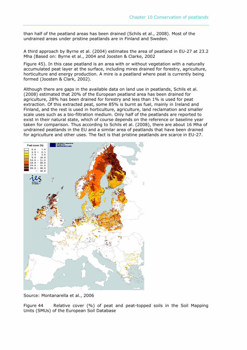
Chapter 10 Conservation of peatlands
than half of the peatland areas has been drained (Schils et al., 2008). Most of the undrained areas under pristine peatlands are in Finland and Sweden.
A third approach by Byrne et al. (2004) estimates the area of peatland in EU-27 at 23.2 Mha (Based on: Byrne et al., 2004 and Joosten & Clarke, 2002
Figure 45). In this case peatland is an area with or without vegetation with a naturally accumulated peat layer at the surface, including mires drained for forestry, agriculture, horticulture and energy production. A mire is a peatland where peat is currently being formed (Joosten & Clark, 2002). Although there are gaps in the available data on land use in peatlands, Schils et al. (2008) estimated that 20% of the European peatland area has been drained for agriculture, 28% has been drained for forestry and less than 1% is used for peat extraction. Of this extracted peat, some 85% is burnt as fuel, mainly in Ireland and Finland, and the rest is used in horticulture, agriculture, land reclamation and smaller scale uses such as a bio-filtration medium. Only half of the peatlands are reported to exist in their natural state, which of course depends on the reference or baseline year taken for comparison. Thus according to Schils et al. (2008), there are about 16 Mha of undrained peatlands in the EU and a similar area of peatlands that have been drained for agriculture and other uses. The fact is that pristine peatlands are scarce in EU-27.
Source: Montanarella et al., 2006
Figure 44 Relative cover (%) of peat and peat-topped soils in the Soil Mapping Units (SMUs) of the European Soil Database
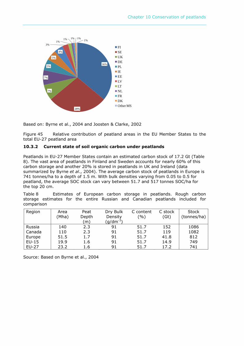
Chapter 10 Conservation of peatlands
36%
28%
7%
7%
5%
5%
4%
3%1%
1% 1% 1%1%
FISEUKDEPLIEEELVLTNLFRDKOther MS
Based on: Byrne et al., 2004 and Joosten & Clarke, 2002
Figure 45 Relative contribution of peatland areas in the EU Member States to the total EU-27 peatland area
10.3.2 Current state of soil organic carbon under peatlands
Peatlands in EU-27 Member States contain an estimated carbon stock of 17.2 Gt (Table 8). The vast area of peatlands in Finland and Sweden accounts for nearly 60% of this carbon storage and another 20% is stored in peatlands in UK and Ireland (data summarized by Byrne et al., 2004). The average carbon stock of peatlands in Europe is 741 tonnes/ha to a depth of 1.5 m. With bulk densities varying from 0.05 to 0.5 for peatland, the average SOC stock can vary between 51.7 and 517 tonnes SOC/ha for the top 20 cm.
Table 8 Estimates of European carbon storage in peatlands. Rough carbon storage estimates for the entire Russian and Canadian peatlands included for comparison
Region Area (Mha)
Peat Depth (m)
Dry Bulk Density (g/dm-3)
C content (%)
C stock (Gt)
Stock (tonnes/ha)
Russia 140 2.3 91 51.7 152 1086 Canada 110 2.3 91 51.7 119 1082 Europe 51.5 1.7 91 51.7 41.8 812 EU-15 19.9 1.6 91 51.7 14.9 749 EU-27 23.2 1.6 91 51.7 17.2 741
Source: Based on Byrne et al., 2004
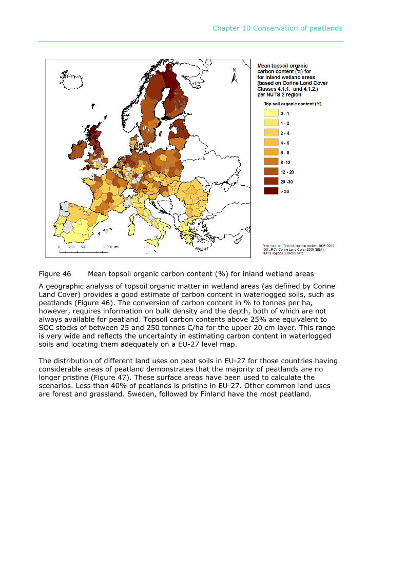
Chapter 10 Conservation of peatlands
Figure 46 Mean topsoil organic carbon content (%) for inland wetland areas
A geographic analysis of topsoil organic matter in wetland areas (as defined by Corine Land Cover) provides a good estimate of carbon content in waterlogged soils, such as peatlands (Figure 46). The conversion of carbon content in % to tonnes per ha, however, requires information on bulk density and the depth, both of which are not always available for peatland. Topsoil carbon contents above 25% are equivalent to SOC stocks of between 25 and 250 tonnes C/ha for the upper 20 cm layer. This range is very wide and reflects the uncertainty in estimating carbon content in waterlogged soils and locating them adequately on a EU-27 level map. The distribution of different land uses on peat soils in EU-27 for those countries having considerable areas of peatland demonstrates that the majority of peatlands are no longer pristine (Figure 47). These surface areas have been used to calculate the scenarios. Less than 40% of peatlands is pristine in EU-27. Other common land uses are forest and grassland. Sweden, followed by Finland have the most peatland.
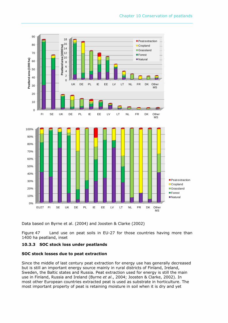
Chapter 10 Conservation of peatlands
0
10
20
30
40
50
60
70
80
90
FI SE UK DE PL IE EE LV LT NL FR DK Other MS
Peat
land
are
a (1
000
ha)
Peat extractionCroplandGrasslandForestNatural
02468
1012141618
UK DE PL IE EE LV LT NL FR DK Other MS
Peat
land
are
a (1
000
ha)
Peat extractionCroplandGrasslandForestNatural
0%
10%
20%
30%
40%
50%
60%
70%
80%
90%
100%
EU27 FI SE UK DE PL IE EE LV LT NL FR DK Other MS
Peat extractionCroplandGrasslandForestNatural
Data based on Byrne et al. (2004) and Joosten & Clarke (2002)
Figure 47 Land use on peat soils in EU-27 for those countries having more than 1400 ha peatland, inset
10.3.3 SOC stock loss under peatlands
SOC stock losses due to peat extraction Since the middle of last century peat extraction for energy use has generally decreased but is still an important energy source mainly in rural districts of Finland, Ireland, Sweden, the Baltic states and Russia. Peat extraction used for energy is still the main use in Finland, Russia and Ireland (Byrne et al., 2004; Joosten & Clarke, 2002). In most other European countries extracted peat is used as substrate in horticulture. The most important property of peat is retaining moisture in soil when it is dry and yet
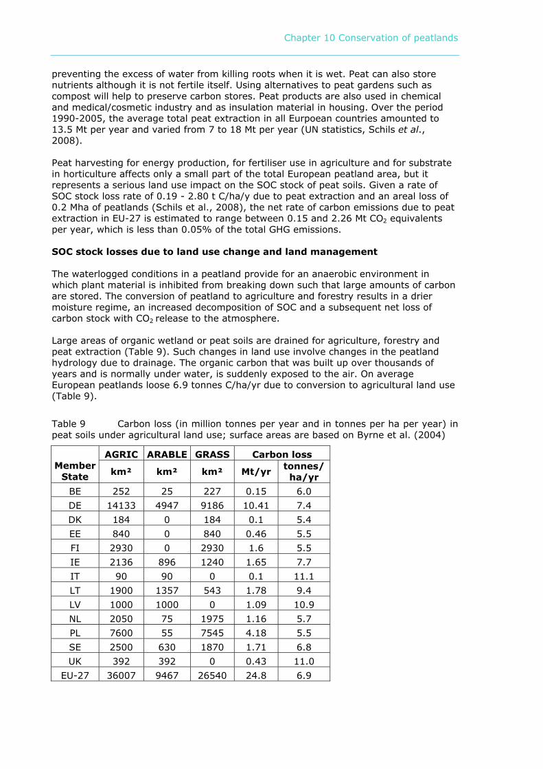
Chapter 10 Conservation of peatlands
preventing the excess of water from killing roots when it is wet. Peat can also store nutrients although it is not fertile itself. Using alternatives to peat gardens such as compost will help to preserve carbon stores. Peat products are also used in chemical and medical/cosmetic industry and as insulation material in housing. Over the period 1990-2005, the average total peat extraction in all Eurpoean countries amounted to 13.5 Mt per year and varied from 7 to 18 Mt per year (UN statistics, Schils et al., 2008). Peat harvesting for energy production, for fertiliser use in agriculture and for substrate in horticulture affects only a small part of the total European peatland area, but it represents a serious land use impact on the SOC stock of peat soils. Given a rate of SOC stock loss rate of 0.19 - 2.80 t C/ha/y due to peat extraction and an areal loss of 0.2 Mha of peatlands (Schils et al., 2008), the net rate of carbon emissions due to peat extraction in EU-27 is estimated to range between 0.15 and 2.26 Mt CO2 equivalents per year, which is less than 0.05% of the total GHG emissions. SOC stock losses due to land use change and land management The waterlogged conditions in a peatland provide for an anaerobic environment in which plant material is inhibited from breaking down such that large amounts of carbon are stored. The conversion of peatland to agriculture and forestry results in a drier moisture regime, an increased decomposition of SOC and a subsequent net loss of carbon stock with CO2 release to the atmosphere. Large areas of organic wetland or peat soils are drained for agriculture, forestry and peat extraction (Table 9). Such changes in land use involve changes in the peatland hydrology due to drainage. The organic carbon that was built up over thousands of years and is normally under water, is suddenly exposed to the air. On average European peatlands loose 6.9 tonnes C/ha/yr due to conversion to agricultural land use (Table 9).
Table 9 Carbon loss (in million tonnes per year and in tonnes per ha per year) in peat soils under agricultural land use; surface areas are based on Byrne et al. (2004)
AGRIC ARABLE GRASS Carbon loss Member
State km² km² km² Mt/yr tonnes/ha/yr
BE 252 25 227 0.15 6.0 DE 14133 4947 9186 10.41 7.4 DK 184 0 184 0.1 5.4 EE 840 0 840 0.46 5.5 FI 2930 0 2930 1.6 5.5 IE 2136 896 1240 1.65 7.7 IT 90 90 0 0.1 11.1 LT 1900 1357 543 1.78 9.4 LV 1000 1000 0 1.09 10.9 NL 2050 75 1975 1.16 5.7 PL 7600 55 7545 4.18 5.5 SE 2500 630 1870 1.71 6.8 UK 392 392 0 0.43 11.0
EU-27 36007 9467 26540 24.8 6.9
Chapter 10 Conservation of peatlands
SOC stock losses due to natural hazards Peat can easily burn under low moisture conditions. Peat fires are often smouldering fires that can burn undetected for very long periods of time. C loss rates due to burning were estimated at 0.26 t C/ha/y for EU-27 (peat surface and above-ground biomass loss). The 2010 Russian peat fires, caused by an unusually high heat wave, were responsible for covering Moscow with a toxic blanket of smog.
10.4 Soil organic carbon fluxes under peatland
The main processes affecting the carbon balance of peatlands are carbon accumulation due to peat formation, extraction due to human activity and losses due to conversion to different types of land use (unmanaged or natural peatlands, forests, grassland, arable land). Exploitation of peatlands for forestry, agriculture or peat extraction involves drainage of peatlands. As a result, the drained peat layer undergoes oxidation resulting in emissions of CO2. 10.4.1 Positive SOC fluxes under peatland
In a natural state, peatlands accumulate carbon because the rate of biomass production is greater than the rate of decomposition. The accumulation of peat involves an interaction between plant productivity and carbon losses through the process of decay, leaching, peat fires and deposition of carbon into the mineral soil beneath peat layers. Most peat-forming systems consist of two layers: an upper aerobic layer of high hydraulic conductivity in which the rate of decay is high; and the predominantly anaerobic underlying layer of low hydraulic conductivity with a lower rate of decay. The boundary between these layers is approximately at the mean depth of the minimum water table in summer (Clymo, 1983, 1984; Joosten & Clarke, 2002). Carbon is added to the surface of the peat through net primary production. Depending on the peat type and decay rates, carbon accumulation in boreal regions ranges from 0.10 to 3.0 t C/ ha/y (Tolonen & Turunen, 1996). Boreal regions of the EU include most of Sweden and Finland, all of Estonia, Latvia and Lithuania and much of the Baltic Sea (Sundseth, K. 2009). The recent rate of carbon accumulation normally refers to young peat layers some hundreds of years old. The long-term apparent rate of C accumulation (LORCA) throughout the Holocene is calculated from the profile of dry bulk density from surface to bottom of the peat layer. Estimates for LORCA in Finland, Russia and Sweden (Byrne et al.,2004) were in the range of 0.15-0.25 t C/ha/y. Cannell et al. (1999) estimated accumulation rates in UK peatlands at 0.20 - 0.50 t C/ha/y. The true net rate of C accumulation (ARCA) can be determined by peat accumulation models, and has been estimated at 2/3 of LORCA (Tolonen & Turunen, 1996). Given an ARCA range of 0.100 - 0.333 t C/ha/y (2/3 of the LORCA range 15-50 t C/ha/y) and 31.8 Mha of peatlands, the net rate of carbon accumulation in EU-27 is estimated to range between 11 and 38 Mt CO2 equivalents per year, which is less than 1% of the total GHG emissions. 10.4.2 Negative carbon fluxes for peatland
Historically, northern peatlands have functioned as a carbon sink, sequestering large amounts of soil organic carbon, mainly due to low decomposition in cold, largely waterlogged soils. Because of the high water-holding capacity of peat and its low hydraulic conductivity, accumulation of soil organic carbon raises the water table, which lowers decomposition rates of soil organic carbon in a positive feedback loop in a two-way interaction between hydrology and biogeochemistry. The feedback between the water table and peat depth increases the sensitivity of peat decomposition to temperature, and intensifies the loss of soil organic carbon in a changing climate (Ise et
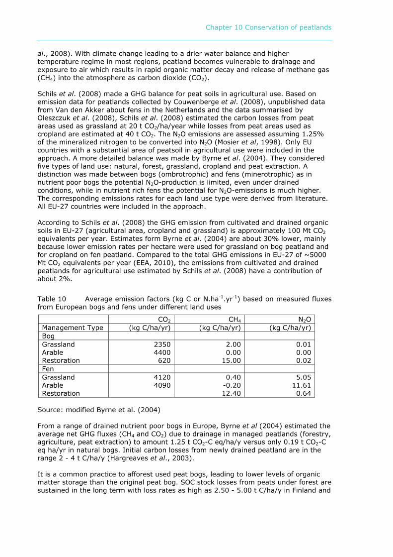
Chapter 10 Conservation of peatlands
al., 2008). With climate change leading to a drier water balance and higher temperature regime in most regions, peatland becomes vulnerable to drainage and exposure to air which results in rapid organic matter decay and release of methane gas (CH4) into the atmosphere as carbon dioxide (CO2). Schils et al. (2008) made a GHG balance for peat soils in agricultural use. Based on emission data for peatlands collected by Couwenberge et al. (2008), unpublished data from Van den Akker about fens in the Netherlands and the data summarised by Oleszczuk et al. (2008), Schils et al. (2008) estimated the carbon losses from peat areas used as grassland at 20 t CO2/ha/year while losses from peat areas used as cropland are estimated at 40 t CO2. The N2O emissions are assessed assuming 1.25% of the mineralized nitrogen to be converted into N2O (Mosier et al, 1998). Only EU countries with a substantial area of peatsoil in agricultural use were included in the approach. A more detailed balance was made by Byrne et al. (2004). They considered five types of land use: natural, forest, grassland, cropland and peat extraction. A distinction was made between bogs (ombrotrophic) and fens (minerotrophic) as in nutrient poor bogs the potential N2O-production is limited, even under drained conditions, while in nutrient rich fens the potential for N2O-emissions is much higher. The corresponding emissions rates for each land use type were derived from literature. All EU-27 countries were included in the approach. According to Schils et al. (2008) the GHG emission from cultivated and drained organic soils in EU-27 (agricultural area, cropland and grassland) is approximately 100 Mt CO2 equivalents per year. Estimates form Byrne et al. (2004) are about 30% lower, mainly because lower emission rates per hectare were used for grassland on bog peatland and for cropland on fen peatland. Compared to the total GHG emissions in EU-27 of ~5000 Mt CO2 equivalents per year (EEA, 2010), the emissions from cultivated and drained peatlands for agricultural use estimated by Schils et al. (2008) have a contribution of about 2%.
Table 10 Average emission factors (kg C or N.ha-1.yr-1) based on measured fluxes from European bogs and fens under different land uses
CO2 CH4 N2O Management Type (kg C/ha/yr) (kg C/ha/yr) (kg C/ha/yr) Bog Grassland Arable Restoration
23504400620
2.000.00
15.00
0.01 0.00 0.02
Fen Grassland Arable Restoration
41204090
0.40-0.2012.40
5.05 11.61 0.64
Source: modified Byrne et al. (2004) From a range of drained nutrient poor bogs in Europe, Byrne et al (2004) estimated the average net GHG fluxes (CH4 and CO2) due to drainage in managed peatlands (forestry, agriculture, peat extraction) to amount 1.25 t CO2-C eq/ha/y versus only 0.19 t CO2-C eq ha/yr in natural bogs. Initial carbon losses from newly drained peatland are in the range 2 - 4 t C/ha/y (Hargreaves et al., 2003). It is a common practice to afforest used peat bogs, leading to lower levels of organic matter storage than the original peat bog. SOC stock losses from peats under forest are sustained in the long term with loss rates as high as 2.50 - 5.00 t C/ha/y in Finland and
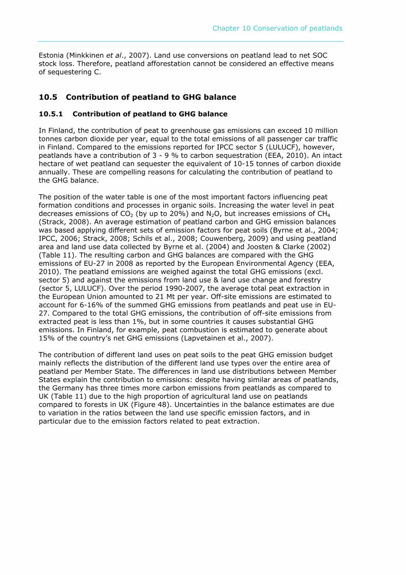
Chapter 10 Conservation of peatlands
Estonia (Minkkinen et al., 2007). Land use conversions on peatland lead to net SOC stock loss. Therefore, peatland afforestation cannot be considered an effective means of sequestering C.
10.5 Contribution of peatland to GHG balance
10.5.1 Contribution of peatland to GHG balance
In Finland, the contribution of peat to greenhouse gas emissions can exceed 10 million tonnes carbon dioxide per year, equal to the total emissions of all passenger car traffic in Finland. Compared to the emissions reported for IPCC sector 5 (LULUCF), however, peatlands have a contribution of 3 - 9 % to carbon sequestration (EEA, 2010). An intact hectare of wet peatland can sequester the equivalent of 10-15 tonnes of carbon dioxide annually. These are compelling reasons for calculating the contribution of peatland to the GHG balance. The position of the water table is one of the most important factors influencing peat formation conditions and processes in organic soils. Increasing the water level in peat decreases emissions of CO2 (by up to 20%) and N2O, but increases emissions of CH4 (Strack, 2008). An average estimation of peatland carbon and GHG emission balances was based applying different sets of emission factors for peat soils (Byrne et al., 2004; IPCC, 2006; Strack, 2008; Schils et al., 2008; Couwenberg, 2009) and using peatland area and land use data collected by Byrne et al. (2004) and Joosten & Clarke (2002) (Table 11). The resulting carbon and GHG balances are compared with the GHG emissions of EU-27 in 2008 as reported by the European Environmental Agency (EEA, 2010). The peatland emissions are weighed against the total GHG emissions (excl. sector 5) and against the emissions from land use & land use change and forestry (sector 5, LULUCF). Over the period 1990-2007, the average total peat extraction in the European Union amounted to 21 Mt per year. Off-site emissions are estimated to account for 6-16% of the summed GHG emissions from peatlands and peat use in EU-27. Compared to the total GHG emissions, the contribution of off-site emissions from extracted peat is less than 1%, but in some countries it causes substantial GHG emissions. In Finland, for example, peat combustion is estimated to generate about 15% of the country’s net GHG emissions (Lapvetainen et al., 2007). The contribution of different land uses on peat soils to the peat GHG emission budget mainly reflects the distribution of the different land use types over the entire area of peatland per Member State. The differences in land use distributions between Member States explain the contribution to emissions: despite having similar areas of peatlands, the Germany has three times more carbon emissions from peatlands as compared to UK (Table 11) due to the high proportion of agricultural land use on peatlands compared to forests in UK (Figure 48). Uncertainties in the balance estimates are due to variation in the ratios between the land use specific emission factors, and in particular due to the emission factors related to peat extraction.
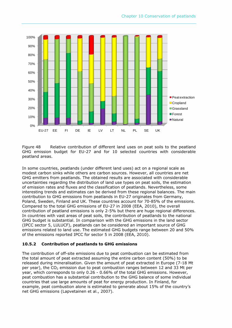
Chapter 10 Conservation of peatlands
0%
10%
20%
30%
40%
50%
60%
70%
80%
90%
100%
EU-27 EE FI DE IE LV LT NL PL SE UK
Peat extractionCroplandGrasslandForestNatural
Figure 48 Relative contribution of different land uses on peat soils to the peatland GHG emission budget for EU-27 and for 10 selected countries with considerable peatland areas.
In some countries, peatlands (under different land uses) act on a regional scale as modest carbon sinks while others are carbon sources. However, all countries are net GHG emitters from peatlands. The obtained results are associated with considerable uncertainties regarding the distribution of land use types on peat soils, the estimation of emission rates and fluxes and the classification of peatlands. Nevertheless, some interesting trends and estimates can be derived from these regional balances. The main contribution to GHG emissions from peatlands in EU-27 originates from Germany, Poland, Sweden, Finland and UK. These countries account for 70-85% of the emissions. Compared to the total GHG emissions of EU-27 in 2008 (EEA, 2010), the overall contribution of peatland emissions is only 2-5% but there are huge regional differences. In countries with vast areas of peat soils, the contribution of peatlands to the national GHG budget is substantial. In comparison with the GHG emissions in the land sector (IPCC sector 5, LULUCF), peatlands can be considered an important source of GHG emissions related to land use. The estimated GHG budgets range between 20 and 50% of the emissions reported IPCC for sector 5 in 2008 (EEA, 2010). 10.5.2 Contribution of peatlands to GHG emissions
The contribution of off-site emissions due to peat combustion can be estimated from the total amount of peat extracted assuming the entire carbon content (50%) to be released during mineralisation. Given the amount of peat extracted in Europe (7-18 Mt per year), the CO2 emission due to peat combustion ranges between 12 and 33 Mt per year, which corresponds to only 0.26 - 0.66% of the total GHG emissions. However, peat combustion has a substantial contribution to the GHG balance of some individual countries that use large amounts of peat for energy production. In Finland, for example, peat combustion alone is estimated to generate about 15% of the country’s net GHG emissions (Lapvetainen et al., 2007).
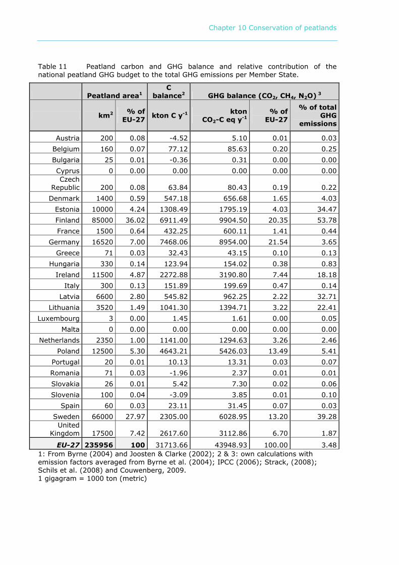
Chapter 10 Conservation of peatlands
Table 11 Peatland carbon and GHG balance and relative contribution of the national peatland GHG budget to the total GHG emissions per Member State.
Peatland area1 C
balance2 GHG balance (CO2, CH4, N2O) 3
km2 % of EU-27 kton C y-1 kton
CO2-C eq y-1 % of EU-27
% of total GHG
emissions
Austria 200 0.08 -4.52 5.10 0.01 0.03Belgium 160 0.07 77.12 85.63 0.20 0.25Bulgaria 25 0.01 -0.36 0.31 0.00 0.00Cyprus 0 0.00 0.00 0.00 0.00 0.00Czech
Republic 200 0.08 63.84 80.43 0.19 0.22Denmark 1400 0.59 547.18 656.68 1.65 4.03
Estonia 10000 4.24 1308.49 1795.19 4.03 34.47Finland 85000 36.02 6911.49 9904.50 20.35 53.78France 1500 0.64 432.25 600.11 1.41 0.44
Germany 16520 7.00 7468.06 8954.00 21.54 3.65Greece 71 0.03 32.43 43.15 0.10 0.13
Hungaria 330 0.14 123.94 154.02 0.38 0.83Ireland 11500 4.87 2272.88 3190.80 7.44 18.18
Italy 300 0.13 151.89 199.69 0.47 0.14Latvia 6600 2.80 545.82 962.25 2.22 32.71
Lithuania 3520 1.49 1041.30 1394.71 3.22 22.41Luxembourg 3 0.00 1.45 1.61 0.00 0.05
Malta 0 0.00 0.00 0.00 0.00 0.00Netherlands 2350 1.00 1141.00 1294.63 3.26 2.46
Poland 12500 5.30 4643.21 5426.03 13.49 5.41Portugal 20 0.01 10.13 13.31 0.03 0.07Romania 71 0.03 -1.96 2.37 0.01 0.01Slovakia 26 0.01 5.42 7.30 0.02 0.06Slovenia 100 0.04 -3.09 3.85 0.01 0.10
Spain 60 0.03 23.11 31.45 0.07 0.03Sweden 66000 27.97 2305.00 6028.95 13.20 39.28United
Kingdom 17500 7.42 2617.60 3112.86 6.70 1.87
EU-27 235956 100 31713.66 43948.93 100.00 3.481: From Byrne (2004) and Joosten & Clarke (2002); 2 & 3: own calculations with emission factors averaged from Byrne et al. (2004); IPCC (2006); Strack, (2008); Schils et al. (2008) and Couwenberg, 2009. 1 gigagram = 1000 ton (metric)
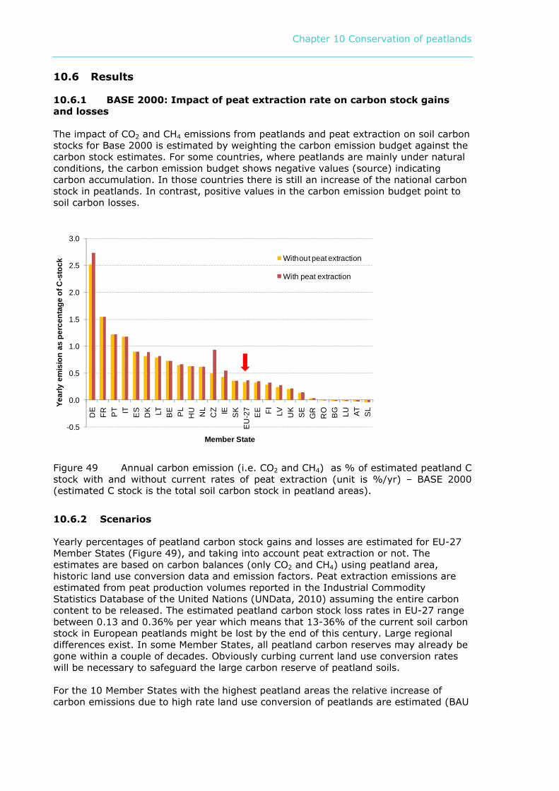
Chapter 10 Conservation of peatlands
10.6 Results
10.6.1 BASE 2000: Impact of peat extraction rate on carbon stock gains and losses
The impact of CO2 and CH4 emissions from peatlands and peat extraction on soil carbon stocks for Base 2000 is estimated by weighting the carbon emission budget against the carbon stock estimates. For some countries, where peatlands are mainly under natural conditions, the carbon emission budget shows negative values (source) indicating carbon accumulation. In those countries there is still an increase of the national carbon stock in peatlands. In contrast, positive values in the carbon emission budget point to soil carbon losses.
-0.5
0.0
0.5
1.0
1.5
2.0
2.5
3.0
DE
FR PT IT ES
DK LT BE PL
HU NL
CZ IE SK
EU
-27
EE FI LV UK
SE
GR
RO BG LU AT SLYe
arly
em
isio
n as
per
cent
age
of C
-sto
ck
Member State
Without peat extraction
With peat extraction
Figure 49 Annual carbon emission (i.e. CO2 and CH4) as % of estimated peatland C stock with and without current rates of peat extraction (unit is %/yr) – BASE 2000 (estimated C stock is the total soil carbon stock in peatland areas).
10.6.2 Scenarios
Yearly percentages of peatland carbon stock gains and losses are estimated for EU-27 Member States (Figure 49), and taking into account peat extraction or not. The estimates are based on carbon balances (only CO2 and CH4) using peatland area, historic land use conversion data and emission factors. Peat extraction emissions are estimated from peat production volumes reported in the Industrial Commodity Statistics Database of the United Nations (UNData, 2010) assuming the entire carbon content to be released. The estimated peatland carbon stock loss rates in EU-27 range between 0.13 and 0.36% per year which means that 13-36% of the current soil carbon stock in European peatlands might be lost by the end of this century. Large regional differences exist. In some Member States, all peatland carbon reserves may already be gone within a couple of decades. Obviously curbing current land use conversion rates will be necessary to safeguard the large carbon reserve of peatland soils. For the 10 Member States with the highest peatland areas the relative increase of carbon emissions due to high rate land use conversion of peatlands are estimated (BAU
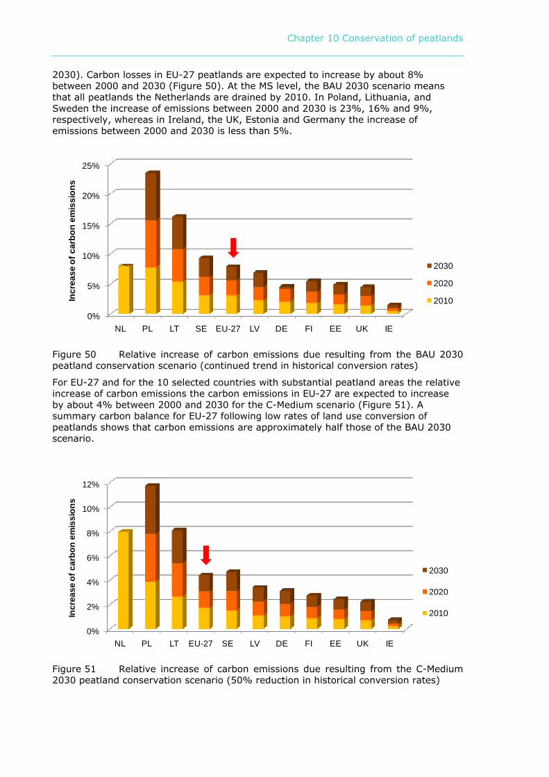
Chapter 10 Conservation of peatlands
2030). Carbon losses in EU-27 peatlands are expected to increase by about 8% between 2000 and 2030 (Figure 50). At the MS level, the BAU 2030 scenario means that all peatlands the Netherlands are drained by 2010. In Poland, Lithuania, and Sweden the increase of emissions between 2000 and 2030 is 23%, 16% and 9%, respectively, whereas in Ireland, the UK, Estonia and Germany the increase of emissions between 2000 and 2030 is less than 5%.
0%
5%
10%
15%
20%
25%
NL PL LT SE EU-27 LV DE FI EE UK IE
Incr
ease
of c
arbo
n em
issi
ons
2030
2020
2010
Figure 50 Relative increase of carbon emissions due resulting from the BAU 2030 peatland conservation scenario (continued trend in historical conversion rates)
For EU-27 and for the 10 selected countries with substantial peatland areas the relative increase of carbon emissions the carbon emissions in EU-27 are expected to increase by about 4% between 2000 and 2030 for the C-Medium scenario (Figure 51). A summary carbon balance for EU-27 following low rates of land use conversion of peatlands shows that carbon emissions are approximately half those of the BAU 2030 scenario.
0%
2%
4%
6%
8%
10%
12%
NL PL LT EU-27 SE LV DE FI EE UK IE
Incr
ease
of c
arbo
n em
issi
ons
2030
2020
2010
Figure 51 Relative increase of carbon emissions due resulting from the C-Medium 2030 peatland conservation scenario (50% reduction in historical conversion rates)
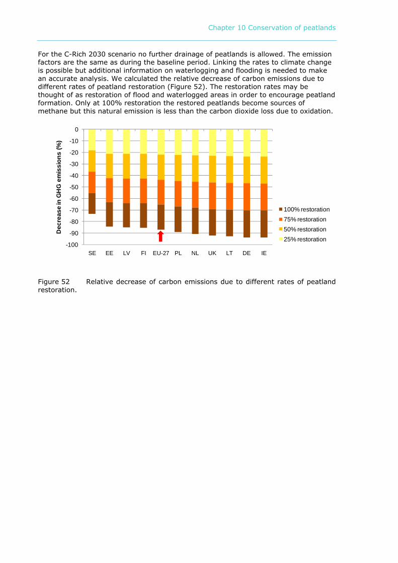
Chapter 10 Conservation of peatlands
For the C-Rich 2030 scenario no further drainage of peatlands is allowed. The emission factors are the same as during the baseline period. Linking the rates to climate change is possible but additional information on waterlogging and flooding is needed to make an accurate analysis. We calculated the relative decrease of carbon emissions due to different rates of peatland restoration (Figure 52). The restoration rates may be thought of as restoration of flood and waterlogged areas in order to encourage peatland formation. Only at 100% restoration the restored peatlands become sources of methane but this natural emission is less than the carbon dioxide loss due to oxidation.
-100
-90
-80
-70
-60
-50
-40
-30
-20
-10
0
SE EE LV FI EU-27 PL NL UK LT DE IE
Dec
reas
e in
GH
G e
mis
sion
s (%
)
100% restoration75% restoration50% restoration25% restoration
Figure 52 Relative decrease of carbon emissions due to different rates of peatland restoration.

Chapter 10 Conservation of peatlands