Chapter--7777 Pricing and Hedging Performance of thethe BS ...shodhganga.inflibnet.ac.in/bitstream/10603/31751/12/12_chapter 7.pdf · Chapter-7 Pricing and Hedging Performance of

ChapterChapterChapterChapter----7777

Pricing and Hedging Performance of Pricing and Hedging Performance of Pricing and Hedging Performance of Pricing and Hedging Performance of thethethethe BS BS BS BS ModelModelModelModel

Chapter-7 Pricing and Hedging Performance of the BS Model

304

CHAPTER-7

PRICING AND HEDGING PERFORMANCE OF THE

BS MODEL

The celebrated Black and Scholes (BS) model has been a very effective tool for both the

valuation and risk management of derivative assets. This is inspite of an overwhelming

body of empirical evidence that refutes to a greater or lesser degree the strict assumptions

underlying the model and comes out with different refinements, extensions and

alternatives to the BS model (as discussed in chapter two). But perhaps it is exactly this

overwhelming body of empirical evidence that leaves the BS model alive today. It is the

only model that every participant in the financial markets understands and every

researcher includes it as a benchmark model with which to compare his/her research. No

other single model is as widely used, understood and compared with, as the BS model

and all the various alternatives developed, of which there are bewilderingly many, have

their own particular strengths and weaknesses. The present chapter performs various

empirical tests on the BS model to know how well it performs in pricing the option

contracts as well as to know its hedging performance in India. There are six sections in

the chapter: the first section deals with some basic description of the options data

included in the empirical tests; the second section includes the procedures involved in

estimating various variables that will be used as inputs into the BS model; the third

section analyses the BS model’s misspecification through the implied volatility graph;

the fourth section performs an empirical test to highlight model’s misspecification as is

indicated by its pricing errors with different volatility inputs; the fifth section describes

the empirical tests conducted to know the model’s hedging performances with different

volatility inputs; and the last section summarizes the whole chapter.

7.1. DATA DESCRIPTION

7.1.1. Nifty Index Options Contracts

(1) S&P CNX Nifty

S&P CNX Nifty is a market- value-weighted index of 50 major stocks i.e. it is

calculated through the market capitalization weighted method. In this method, the


305

equity price is weighted by the market capitalization of the company (share price x

number of outstanding shares). Hence each constituent stock in the index affects the

index value in the proportion to the market value of all the outstanding shares. In this

method index is calculated as:

)(

)(

b

c

MtioncapitalisamarketBase

valueBasexMtioncapitalisamarketCurrentIndex = [7.1]

where

cM = Sum of (current market price x outstanding shares) of all securities in the index.

bM = Sum of (market price x issue size) of all securities as on the base date.

The base period selected for Nifty is the closing prices on November3, 1995. The base

value of the index has been set at 1000 and a base capital of Rs. 2.06 trillion.

(2) Nifty Option Contracts

First index option was launched in India on June 4, 2001. For Nifty option contracts,

exercise style is European style (while for option contracts on individual securities

exercise style is American style). Final exercise is automatic on expiry of the option

contract. The expiry day is last Thursday of the expiry month. If it is a holiday then

expiry day is previous trading day. The lot size of option contracts is 200 and multiple

thereof. In other words, when index stands at 1010, Rs. 202000 worth of underlying

stocks are controlled by a single option contract. The price steps in respect of Nifty

option contracts are 0.05, whereas the strike price interval is 10. The option contract (as

indeed with most of the index option contracts) has cash settlement so that a writer, on

being assigned an exercise of a call, delivers in cash the difference between the index

value and the exercise price.

7.1.2. Data

This study uses S&P CNX Nifty call options for analysis as these are European style

contracts which fits in the assumptions of the basic BS model studied here. More so, the

dividend yield on Nifty is available on the National Stock Exchange (NSE) site. Since

we have seen in the previous chapter that the out-of-sample period for which the


306

volatilities through the various models are forecasted spans from July 1, 2008 to June

30, 2011, therefore the BS model is tested by applying it on Nifty for the same period.

In other words the data taken for Nifty options is from July1, 2008 through June 30,

2011. The option premiums, Nifty index close prices and the dividend yield on Nifty

are obtained from NSE site (www.nseindia.com). Figure 7.1 below shows the

performance of the underlying index i.e Nifty for the whole period of the study.

Figure 7.1: Nifty Index Level

It is to be noted that, since the quotes for Nifty are taken as the closing prices rather

than the corresponding index level at the moment when the option prices are recorded,

it may introduce non-synchronous price problems. In other words, the closing option

prices and closing Nifty prices may not be prices that prevailed simultaneously because

the last option trade might have been early in the day while last Nifty trade is close to

end of the day. Moreover, if trading in options is thin on a given day, then it means that

the closing prices of many options came from trades done several hours before close.

So thin trading in options worsens the non-simultaneous pricing problem.

At any point of time, there are short term, medium term and long term options available

for trading. These contracts expire on last Thursday of the expiry month. If the last

Thursday is a trading holiday; the contracts expire on the previous trading day. A new

0

1000

2000

3000

4000

5000

6000

7000

1-Jul-02 1-Jul-03 1-Jul-04 1-Jul-05 1-Jul-06 1-Jul-07 1-Jul-08 1-Jul-09 1-Jul-10

Pri

ce (

Rs.

)

Year

Nifty Closing Prices


307

contract is introduced on the next trading day following the expiry of the near month

contract. All the derivative contracts are presently cash settled. The long term option

and medium term contracts are available for 3 serial month contracts, 3 quarterly

months of the cycle March / June / September / December and 5 following semi-annual

months of the cycle June / December. Thus, at any point of time, there are at least 3

year tenure options available. Since the trading done in most of the option contracts,

except the one-month options, is very less therefore, the present study concentrates only

on one-month option contracts.

Index options, as compared to equity options are cash settled and physical delivery is

not possible for them. Traders, who want to hedge can use proxy portfolios that mimic

the Index so as to enable physical delivery of the securities included in the portfolio. To

conduct empirical tests previous researches have used futures prices instead of options

prices to deal with the problem. But since using future prices require usage of a futures

formula into the methodology, therefore to keep things simple, the present study uses

option prices instead of future prices. Moreover, since creation of proxy portfolios is a

much complex process, therefore, we also exclude usage of these portfolios in our

study.

7.2. VARIOUS INPUT CALCULATIONS

A trader requires six inputs to calculate value of an option contract on Index from the

BS model, namely, closing prices of the Index (after adjusting for dividends), dividends

paid on the Index, the strike price of the option, time to maturity of the option, interest

rates and volatility of the index. These input calculations are discussed as follows; but

before this is done one must apply certain exclusion criterion on the data involved for

excluding the outliers from the data.

Exclusion of Outliers

Several exclusion criteria were imposed on the option pricing data. Firstly, fewer than six

days to maturity are eliminated. Short term options are extremely sensitive to non-

synchronous price issues. Secondly, options with absolute moneyness [ ]1)/( −−− rtdt XeSe ,


308

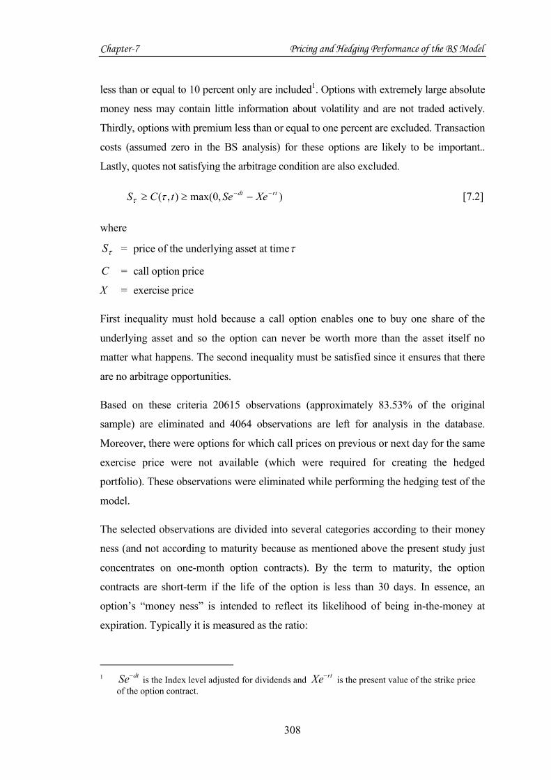
less than or equal to 10 percent only are included1. Options with extremely large absolute

money ness may contain little information about volatility and are not traded actively.

Thirdly, options with premium less than or equal to one percent are excluded. Transaction

costs (assumed zero in the BS analysis) for these options are likely to be important..

Lastly, quotes not satisfying the arbitrage condition are also excluded.

),0max(),( rtdt XeSetCS −− −≥≥ ττ [7.2]

where

τS

= price of the underlying asset at timeτ

C = call option price

X = exercise price

First inequality must hold because a call option enables one to buy one share of the

underlying asset and so the option can never be worth more than the asset itself no

matter what happens. The second inequality must be satisfied since it ensures that there

are no arbitrage opportunities.

Based on these criteria 20615 observations (approximately 83.53% of the original

sample) are eliminated and 4064 observations are left for analysis in the database.

Moreover, there were options for which call prices on previous or next day for the same

exercise price were not available (which were required for creating the hedged

portfolio). These observations were eliminated while performing the hedging test of the

model.

The selected observations are divided into several categories according to their money

ness (and not according to maturity because as mentioned above the present study just

concentrates on one-month option contracts). By the term to maturity, the option

contracts are short-term if the life of the option is less than 30 days. In essence, an

option’s “money ness” is intended to reflect its likelihood of being in-the-money at

expiration. Typically it is measured as the ratio:

1

dtSe− is the Index level adjusted for dividends and rtXe− is the present value of the strike price

of the option contract.


309

Money ness = rt

d

Xe

eS t

−

−∗

=A

A

X

S [7.3]

where rteS∗ is the index level adjusted for dividends. A call option is said to be near-the-

money (NTM) if it’s SA/XA ∈ (0.97-1.03), out-of-the-money (OTM) if SA/XA ≤ 0.97 and

in-the-money (ITM) if SA/XA ≥ 1.03. A finer partition resulted in six money ness

categories for which the results will be reported. Table 7.1 describes certain sample

properties of the Nifty call prices used in the study. Summary statistics are reported for the

average call prices and the total number of observations (which are listed in parenthesis),

for each money ness category. The sample period extends from 1 July, 2008 through 30

June, 2011 for a total of 4064 calls. SA denotes the Nifty index level adjusted for dividends

and XA is the present value of the exercise price. OTM stands for out-of-the-money options,

NTM stands for near-the-money options and ITM stands for in-the-money options. There

are a total of 4064 call option observations, with OTM, ITM and NTM options respectively

taking 13.17 %, 46.11% and 40.72% of the total sample and the average price ranges from

Rs. 57.43 for short-term, deep OTM options to Rs. 379.75 for deep ITM calls. The average

price based on all the options in the out-of-sample period is Rs. 207.93.

Table 7.1: Average Call Prices and Number of Observations

Money ness

(AA XS / )

Average Price

(No. of observations)

OTM

<0.94 57.43

(186)

0.94-0.97 71.63

(349)

NTM

0.97-1.00 94.30

(696)

1.00-1.03 150.14

(959)

ITM

1.03-1.06 251.46

(874)

>1.06 379.75

(1000)

7.2.1. Closing Prices (Adjusted for Dividends) of Nifty

Stocks usually pay dividends on a quarterly basis, at fairly set intervals, so that

calculating the present value of a stock’s dividend stream over the next three or six


310

months is a fairly straight forward operation. When pricing Index options, one must

take into account the dividends paid by all of the component stocks during the life of

the option. Take the Standard & Poor’s 100 Index as an example. One hundred

component stocks means a potential 100 ex-dividend dates every quarter, an average of

more than one per trading day. A relatively unsophisticated way of calculating the

theoretical value of Index options would be to assume a constant, even flow of

dividends throughout the quarter. But this assumption is obviously false; the dividend

rates of the component stocks are not equal, and there are periods during the quarter of

‘heavy dividends’ during which a disproportionately high number of the component

stocks goes ex-dividends.

Calculating the present value of the dividend stream over the life of an Index option

becomes a much more involved process. One must determine which stocks will go ex,

on which dates and by what amounts. What one must calculate is therefore the yield of

the Index from today to a specific option’s expiration date. This yield will not be the

same for different expiration dates and will have to be recalculated for each trading day

to exclude the stocks that have gone ex on the previous day. The variableδ should be

set equal to the average dividend yield (continuously compounded and annualized)

during the life of the option. A known dividend yield means that the dividend income

forms a constant percentage of the stock price. For a dividend yield ofδ , the stock pays

out δS on each ex-dividend date. In the continuous payment model, dividends are paid

continuously. Such a model approximates a broad- based stock market portfolio in

which some company will pay a dividend nearly every day. The payment of a

continuous dividend yield at rate δ reduces the growth rate of the stock price byδ . In

other words, a stock that grows from S to St with a continuous dividend yield of δ

would grow from S to t

teS δ− without the dividends. The variable δ should be set

equal to the average dividend yield (continuously compounded and annualized) during

the life of the option. For the period when an option is first introduced into the market

and till it matures, the dividend yields on Nifty are averaged. This average is then

assumed to remain constant and known for a particular option during its life. The Nifty

Index prices are then adjusted for this known and constant dividend yield δ through the

formula:


311

t

tA eSS δ−= [7.4]

where

AS = adjusted index level

S = unadjusted index level

δ = continuously compounded known and constant dividend yield on NIFTY

t = time to maturity

7.2.2. Strike Price of the Option

The exercise or the strike price is the price at which the call option contract gets executed.

It is a price, which is well-known by both the buyer and the seller of the option at the time

of entering into the contract. It is one of the variables which is not to be calculated, but

rather observed from the features of the options contract by both the parties.

7.2.3. Time to Maturity

Time to maturity is the time period left in the maturity of the option contract from any

point of time t. For the purpose of applying the BS model in order to calculate the

option prices, the time to maturity variable is expressed in the form of proportion of a

year. Thus, if six months are left to expiry of the contract, then time to maturity is

included as an input into the BS model in the form of the value 0.5. Since it is also well

known variable to both the parties involved in the contract, therefore, it is not to be

calculated, but rather only observed and converted into proportion of a year.

7.2.4. Interest Rate Calculations

Because the Black and Scholes model, uses a risk – free rate of interest , one can use

treasury bill rate as a good estimate. Treasury bills (T-bills) represents the debt issued as

discounted securities by the Government with maturities of one year or less. The 91-

day T- Bills, floated by the Government of India from time to time through Reserve

Bank of India is used as a proxy for the risk-free asset and the adjusted yield to


312

maturity ( YTM) implicit at the cut-off rate of 91day T- Bills auctions is considered as

the return of this asset. T-Bills in India are issued at discount and redeemed at par, the

difference being the ‘interest’ paid. The 91-day T-Bills are issued at a fixed discount

rate of 4% as well as through auctions (so as to fetch market interest rates). Discount

rate on these bills are quoted in auction by the participants and accepted by the

authorities. Such a rate is called the cut-off rate.

The steps involved in calculating the risk- free interest rates can be summarized as:

1. First, we collect the interest rate data for each day in the sample from the Reserve

Bank of India (RBI) site (www.rbi.org.in) which provides the implicit yield-to-

maturity at cut-off price which is a simple annualized rate i.e.

mP

PFry

365×

−= [7.5]

where

yr = rate of interest

F = face value

P = cut- off price ( or price issue)

m = time to maturity of the bill

2. Since the Black and Scholes model uses the continuously compounded risk- free

interest rates to determine the call option value, therefore the simple yield is to

be converted into continuously compounded rate by using the natural log function:

)1ln( yrr +=

where

r = continuously compounded risk-free interest rate.

ln = natural logarithm

yr

= the simple risk-free interest rate.

This continuously compounded rate is calculated for each day for a T-bill

issued on any date till the expiry of the T-bill.


313

3. Lastly, to include these risk less interest rates on T-bills as an input into the Black

and Scholes model, their maturity has to be matched with the maturity date of the

option( for most cases they both will match because both the T-bills and the

options mature on last Thursday of a month). The T-bill whose maturity date

matches with that of the option is then selected and the yield on this T-bill is then

followed till maturity.

7.2.5. Volatility Estimations

The volatility of an asset is a measure of variability of its returns. In the previous

chapter we have already seen how volatility can be calculated through various models

and methods. These previously calculated volatilities will now become an input into the

BS model. But, before becoming an input, these volatilities must be converted into

annualized volatilities since the BS model requires all data in annualized form. The

annualization of the volatility figures can be done through the simple formula:

Daily Annualized Volatility �� √252 [7.6]

7.3. IMPLIED VOLATILITY SMILE

Theoretically, since volatility is a property of the underlying asset it should be

predicted by the pricing formula to be identical for all derivatives based on that same

asset. However, in practice, implied volatility of the underlying asset varies across

various exercise prices and/or time to maturity. Thus market does not price all options

according to Black-Scholes (BS) model. The picture obtained by plotting the implied

volatility with different moneyness (observed at the same time, with similar maturity

and written on the same asset) is known as volatility smiles. Volatility smiles are

generally taken as an indication of misspecification of the model used to calculate

those implied volatilities. The literature is not unanimous in finding the shapes and the

causes of the smile effect. The pattern of IVs across time to expiration is usually

referred to as the term structure of IVs, whereas the 'skew' or the 'smile' refers to the

pattern across moneyness levels. The reason for the expression 'smile' is the empirical

findings for S&P 500 options before the 1987 stock market crash. The IVs for deep


314

in- and out-of-the-money options were found to be higher than the at-the-money

options, thus creating a smile-shaped pattern. After the crash, the smile in S&P 500

options changed to look more like a 'sneer' with monotonically decreasing IV for

increasing exercise prices, but the IV pattern is often referred to as the smile

regardless of its actual shape. The actual shape of the smile differs between different

markets, underlying assets and time periods. For instance, Beber (2001) finds a smile

profile with negative slope for the Italian market, and Engström (2001) reports that

the smile profile is characterized by a positive slope for the Swedish market. Peña,

Rubio, and Serna (1999) show that the smile profile is symmetric in the Spanish

market.

We plot a graph for the implied volatilities, calculated in the previous chapter, against

the different moneyness category of options. The implied volatility graph is given in

figure 7.2.

Figure 7.2: Implied Volatility Smile for the Period 1 July 2008 to 30 June 2011

The horizontal axis includes the moneyness as defined earlier and the vertical axis

includes the average implied volatilities for different categories of moneyness- related

options. As we can see the smile is more of a “smirk” and as one moves from Deep

0

5

10

15

20

25

>0.94 0.97 1 1.03 1.06

Imp

lie

d V

ola

tili

ty (

%)

Moneyness

Implied Volatility Smile


315

OTMs to Deep ITMs, the average implied volatility increases. The NTMs are having

lower volatilities as compared to ITMs and OTMs. The results confirm with other

studies like that by Malabika Deo (2008), etc. The differences in the implied volatilities

indicate that the BS model is misspecified and is based on restrictive assumptions of

constant volatility.

7.4. PRICING PERFORMANCE

Black and Scholes model is often reported to produce model values which differ in

systematic ways from market prices. For example, Black (1975) reports that the model

under prices (overprices) deep out-of-the-money (in-the-money) call options when

standard deviations on the underlying stock are estimated using historical stock price

data. Macbeth and Merville (1979) found biases exactly opposite to those reported by

Black. This section revisits the Black and Scholes model to find biases, if any, by taking

data for call index options, and volatilities calculated from various models as an input

into the BS model, for the period from 1st July 2008 to 30

th June 2011. The efficiency of

an option pricing model is to be tested against a market for options. A problem arises

when efficiency is tested against the market. In such a case, two hypotheses are usually

tested simultaneously: first, that the market is efficient and second, that the model is

efficient; and the test is unable to distinguish between the two hypotheses. Therefore,

researchers assume one to be efficient and test for the efficiency of the other. In the

present study, in testing the BS model’s pricing (as well as hedging performance), we

assume that the Nifty options market is efficient. The null hypothesis tested is that

pricing efficiency of BS model does not depend upon volatility measures.

Methodology and Results

The steps involved in calculating BS model prices can be summarized as follows:

1. Collect information on all the inputs (including the volatilities from different

models implemented in chapter six) required to calculate the BS model prices, as

described previously, on day t.


316

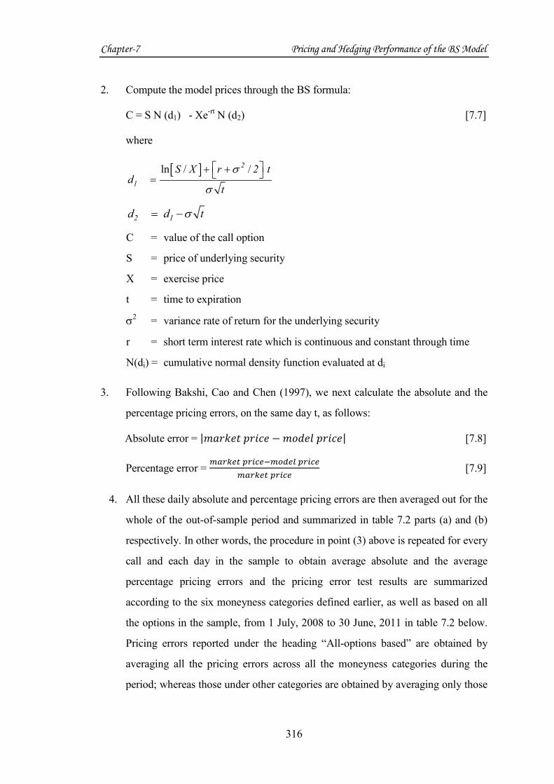
2. Compute the model prices through the BS formula:

C = S N (d1) - Xe-rt

N (d2) [7.7]

where

[ ]ln / /2

1

S X r 2 td

t

σ

σ

+ + =

2 1d d tσ= −

C = value of the call option

S = price of underlying security

X = exercise price

t = time to expiration

σ2 = variance rate of return for the underlying security

r = short term interest rate which is continuous and constant through time

N(di) = cumulative normal density function evaluated at di

3. Following Bakshi, Cao and Chen (1997), we next calculate the absolute and the

percentage pricing errors, on the same day t, as follows:

Absolute error = |� �� | [7.8]

Percentage error = �� !�"#�$ ��

�� [7.9]

4. All these daily absolute and percentage pricing errors are then averaged out for the

whole of the out-of-sample period and summarized in table 7.2 parts (a) and (b)

respectively. In other words, the procedure in point (3) above is repeated for every

call and each day in the sample to obtain average absolute and the average

percentage pricing errors and the pricing error test results are summarized

according to the six moneyness categories defined earlier, as well as based on all

the options in the sample, from 1 July, 2008 to 30 June, 2011 in table 7.2 below.

Pricing errors reported under the heading “All-options based” are obtained by

averaging all the pricing errors across all the moneyness categories during the

period; whereas those under other categories are obtained by averaging only those


317

pricing errors, which lie in a particular moneyness category as defined earlier.

Moneyness (M) is defined as SA/X where SA is the Index level adjusted for

dividends and X is the exercise price. Positive figure shows overpricing and

negative figure shows under pricing. ‘Difference’ in part (a) of the table is the

difference between the best and the worst model in a particular moneyness

category of options

Empirical evidence confirms systematic mispricing of the Black and Scholes call option

pricing model. These biases have been documented with respect to the call option’s

exercise price, its time to maturity, and the underlying asset’s volatility; see for example

Black (1975), Macbeth and Merville (1979), Rubinstein (1985), etc. Various conflicting

patterns of mispricing of the BS model have been documented in the literature. For

example, Black and Scholes themselves admitted in their study in 1972, some biases of

the model, expressed as “Using the past data to estimate the variance caused the model

to overprice options on high variance stocks and underprice options on low variance

stocks. While the model tends to overestimate the value of an option on a high variance

security, market tends to underestimate the value, and similarly while the model tends

to underestimate the value of an option on a low variance security, the market tends to

overestimate the value”. Contrary to this result, Macbeth and Merville (1979) report

that the BS prices, calculated with the implied volatility of at- or near-the-money

options, are on average less (greater) than market prices for ITM (OTM) call options.

These conflicting results may perhaps be reconciled by the fact that the studies

examined market prices at different point of time and these systematic errors vary with

time (Rubinstein (1985). Moreover, the extent to which the BS model under-prices

(overprices) an in-the-money (out-of-the-money) option increases with the extent to

which the option is in-the-money (out-of-the-money) and decreases as time to maturity

decreases.


318

Table 7.2: Pricing Errors for One-Month Nifty Options

(A) Absolute Pricing Errors

Moneyness

Model

All-

options

based

M<0.94 0.9497.0<≤ M

0.97

1<≤M

1 1.03M≤ <

1.03

1.06M≤ <

06.1≥M

RW 46.32 59.72 56.34 58.45 51.57 40.71 31.86

LTM 39.30 53.88 57.01 45.34 36.00 36.57 31.84

MA(15) 28.51 26.21 26.25 29.46 30.36 29.43 26.50

MA(30) 27.47 23.46 24.25 27.66 28.65 29.29 26.49

MA(60) 29.16 31.82 28.33 29.38 29.42 30.47 27.39

EWMA 20.03 23.22 20.88 17.78 17.39 21.28 22.13

SR 31.42 37.56 35.55 38.00 34.25 28.34 24.28

GARCH(11) 21.01 23.20 21.30 19.60 18.16 21.98 23.37

GARCH(42) 21.69 23.77 22.32 20.51 19.30 22.50 23.47

IV 12.98 13.02 10.32 8.71 8.67 15.17 19.06

COMB1 21.82 20.19 20.55 19.29 19.38 24.14 24.64

COMB2 23.34 22.55 23.00 21.47 21.14 25.32 25.27

Difference 33.34 46.7 46.69 49.74 42.9 25.54 12.8

(B) Percentage Pricing Errors

Moneyness

Model

All-

options

based

M<0.94 0.9497.0<≤ M

0.97

1<≤ M

1 1.03M≤ <

1.03

1.06M≤ < 06.1≥M

RW 0.1148 -0.225 0.1525 0.2724 0.1649 0.0724 0.0439

LTM 0.2771 0.9364 0.7880 0.4093 0.1983 0.1379 0.0844

MA(15) 0.1696 0.2580 0.2845 0.2913 0.1936 0.1049 0.0628

MA(30) 0.1721 0.3428 0.2965 0.2857 0.1858 0.1057 0.0638

MA(60) 0.1737 0.4341 0.3060 0.2770 0.1776 0.1054 0.0646

EWMA 0.0121 -0.1671 -0.1269 0.0075 0.0452 0.0442 0.0364

SR 0.0317 0.2835 0.2855 -0.0370 -0.0625 0.0251 0.0412

GARCH(11) 0.0349 -0.0372 0.0136 0.0245 0.0417 0.0505 0.0427

GARCH(42) 0.0390 -0.0160 0.0280 0.0315 0.0425 0.0520 0.0435

IV -0.0038 -0.1584 -0.0883 -0.0444 0.0075 0.0356 0.0363

COMB1 0.1143 0.2464 0.2286 0.1583 0.1043 0.0818 0.0581

COMB2 0.1266 0.2834 0.2612 0.1805 0.1149 0.0864 0.0600

Analysis of the above table shows that in absolute terms the pricing errors are

minimized only when the implied volatility is used as an input into the model. For all

other volatility measures the pricing errors are greater than that for implied volatility.

For example, the absolute errors for call options with moneyness ranging between 1-

1.03, is Rs. 51.57 if random walk model is used, whereas the errors are reduced to


319

Rs. 8.67 when implied volatility is used to value the options. The random walk model is

almost consistently found to be the worst model according to the absolute pricing errors

for all categories of options except for one, that is, for not-so-deep OTMS (for which

LTM is the worst, though very minor difference is there between the performance of

RW and LTM). Moreover, the ‘difference’ heading in table 7.2 part (A) indicates that,

except for one category of options (that is for options with moneyness between 0.97 and

1) as moneyness increases the difference in performance of IV over the worst model

decreases. This can mean that either the relative efficiency of IV model, in enhancing

BS model performance, decreases as moneyness increases, or the efficiency of worst

model, consistently increases as moneyness increases.

If moneyness-wise absolute errors are analyzed, then for the deep OTMs, IV model leads

to minimum absolute errors and the RW model leads to maximum errors by applying the

BS model. The scenario remains almost the same for not-so-deep OTMs with a change

that now LTM is providing the maximum errors. For NTMs and OTMs, RW again is the

worst performer and IV is the best performer. For example, for the NTM calls having

moneyness ranging from 0.97 to 1, maximum absolute errors are Rs. 58.45 (by applying

RW model) which gets reduced to Rs. 8.71 if IV is used as an input to the BS model. In

other words, IV performs best for all the three categories of calls, that is ITM, OTM and

NTMs, and out of these NTMs are having the minimum absolute errors.

Talking in terms of the percentage errors, the random walk model produces 16.49%

errors, which get reduced to 0.75% if the implied volatilities are used to price the calls.

Moreover, the IV model leads to the results, which confirms with the Macbeth and

Merville’s study, that is, the BS model tends to underprice (indicated through negative

percentage errors) OTMs and NTMs and overprices (indicated through positive

percentage errors) ITMs if implied volatilities are used as an input into the model.

Furthermore, according to the percentage errors, the BS model is able to price the deep

ITMs most efficiently out of all the categories of options defined on the basis of

moneyness. For example, from table 7.1, it can be seen that the average price of a deep

ITM is Rs. 379.75. These options are priced with a maximum percentage error of

8.44%, by taking LTM volatility measure as an input to BS model, which are reduced to

3.63% errors by using IV or EWMA models. Whereas the deep OTMs, which are on an


320

average priced as Rs. 57.43, are most inefficiently priced by the BS model, since it

gives a maximum of 93.64% mispricing (as per the LTM model), which is reduced to -

1.6% as per the GARCH (4,2) model.

From amongst all the volatility models, the deep OTMs are underpriced by five models,

namely, RW, EWMA, GARCH(1,1), GARCH(4,2) and the IV model. The other models

overprice the deep OTMs, thus confirming Black’s (1976) result for the same. For the

deep OTMs, it can be seen that the tendency to overprice is more than the tendency to

underprice by the BS model. That is, the positive (thereby indicating overpricing)

percentage errors (in absolute figures) are greater than the negative (thereby indicating

underpricing) percentage errors. For example, the LTM model leads to a maximum of

93.64% overpricing of the deep OTMs, whereas the RW model leads to a maximum of

22.5% underpricing of the deep OTMs. For not-so-deep OTMs the average price is Rs.

71.63 and the maximum percentage error as given by LTM model is 78.80%. Though the

minimum absolute errors are provided by the implied volatility input but the percentage

errors for not-so-deep OTMs are minimized only by the GARCH (1,1) model with 1.3%

errors. This category of options are underpriced only by EWMA and IV models and the

extent to which they are underpriced also decreases as compared to deep OTMs.

Most of the volatility inputs lead to an overpricing of the NTMs except for SR and IV

model. For this category of options, LTM is the worst performer since it leads to pricing

errors of 40.93% and 19.83% for the two sub-categories of NTMs respectively. While

for the NTMs with moneyness between 0.97 and 1, EWMA model proves to be the

best, for the other sub-category of NTMs that is with moneyness between 1 and 1.03,

the IV model proves to be the best. Both models lead to the same amount of percentage

errors of 0.75% for the NTM category of options.

The not-so-deep ITMs are overpriced by all the models. If percentage errors are

considered, then the BS model performs the best with only 2.5% errors if SR model is

used for forecasting volatility. Percentage-wise LTM model performs the worst with

13.79% errors. All volatility models in this category of options perform very closely with

maximum difference of only 11% between the performances (as judged by the percentage

errors) of the models. The deep ITMs are again overpriced by all the volatility inputs and

the maximum overpricing is done by the LTM model whereas minimum being done by


321

IV model. All volatility models in this category of options also perform very closely as

the maximum difference between their performances is to the extent of only 5%.

If we see the model-wise performance, then the RW volatility model leads to the

maximum total absolute errors for almost all categories of options. The percentage

pricing errors decreases from -22.5% (under the deep OTM category) to 4.39% for the

deep ITM category of options. The LTM model is the next worst performer overpricing

all categories of options. The maximum error is 93% for deep OTMs, which get

reduced to 8% for those under the deep ITM category of options.

Under the moving average category of volatility models, all MA models perform very

closely with MA(30) as best performer amongst the MA models in absolute terms.

According to the percentage pricing errors, though, the MA (15) is the best for OTMs and

ITMs whereas MA (60) is the best for NTMs. The three models perform very closely

especially for the ITMs for which the maximum difference between the model’s

performances are 0.2% only. The EWMA model underprices OTMs and overprices the

ITMs and NTMs, whereas the SR model underprices NTMs and overprices ITMs and

OTMs. The simple regression model provides the best performance for not-so-deep ITMs.

Under the GARCH category of models, the two models perform very closely with

GARCH (1,1) model having slightly better performance in absolute terms. Percentage-

wise except for deep OTMs, GARCH (1,1) again is better than GARCH (4,2). The two

models lead to underpricing deep OTMs and overpricing other category of options. The

maximum error between the performances of the two models is not more than 5%. The

IV model provides the same results as that of Macbeth and Merville, that is,

underpricing of OTMs and as moneyness increases it starts leading to overpricing.

Errors range from 15% to less than 1% considering all the categories of options.

Under the combination models, both the models again perform very closely with

COMB1 providing slightly better performance. This indicates that it is better to include

the implied volatility information if one is opting for combination models. This is in

direct contrast to the previous results. Previously, in chapter six, we have seen that

combining implied volatility information decreased the efficiency of the combination

model. But, if the aim of the investor is to price an option, rather than just forecasting


322

volatility, then it is better to combine the implied volatility information into the

combination model. Both the category of combination models overprices all the call

options irrespective of their moneyness, and the percentage errors are maximum for the

OTMs and they start decreasing as the moneyness increases.

In conclusion, firstly, it seems IV model in absolute terms is the best input for the BS

model to price the call options, though it was the worst performer according to the

MAE, MAPE and RMSE statistical measures as was seen in the previous chapter. It

was ranked as the best according to the CDC and MME criterion and in the present

chapter we have seen that if the purpose is to price an option, then the implied volatility

is the best choice as it consistently provides minimum errors irrespective of the

moneyness of a call. And, according to the percentage errors no single model is able to

provide minimized errors consistently throughout all the categories of options.

Secondly, if first nine historical-prices based volatility models are compared (that is

leaving aside IV and the two combination models), there is no single model which

consistently leads to minimized percentage errors for all category of call options,

though GARCH (1,1) and EWMA models are good performers for some category of

options (although in absolute terms barring one exception EWMA is a consistent

performer). RW and LTM consistently provide worst performance across all categories

of call options. Thirdly, it can be seen that ITMs are better priced than OTMs by the BS

model irrespective of the volatility input. Fourthly, no benefits can be gained by

combining models if the purpose of using the volatilities is to price an option. And

lastly, barring a few exceptions, all volatility inputs through the various models in the

BS formula leads to decreased percentage errors as moneyness increases. Moreover, the

null hypothesis that pricing efficiency of the BS model is independent of the volatility

input seems to be rejected by the results.

7.5. HEDGING PERFORMANCE

The key element in the Black and Scholes model is that the return from a risk less

portfolio, consisting of a position in the option and a position in the underlying stock,

must be the risk free interest rate. This single principle results in a differential equation

that must be satisfied by the option. Only one formula for the value of the option has

this property where the return on a continually hedged position of option and stock


323

equals the risk less interest rate. The reason why a risk less portfolio can be set up is

that the stock price and the option price are both affected by the same underlying source

of uncertainty: the stock price movements. So, when an appropriate portfolio of the

stock and option is set up, the gain/loss from stock position will always affect the

gain/loss from the option position. In the absence of arbitrage opportunities, the return

from the portfolio must be the risk free interest rate. If the market price of the call is not

equal to the BS equilibrium price, then an arbitrage return could be earned from the

arbitrage/hedging portfolio. In an efficient market, these arbitrage returns could not be

earned and option prices equate to their true or theoretical values.

The present section tries to determine whether or not excess returns can be earned by

employing the arbitrage trading strategies that underlie the BS model. In conducting

empirical tests of the Black and Scholes model, researchers need to consider whether

the market is truly efficient or not. Significant differences between actual call prices and

the model prices don’t necessarily invalidate the BS model, since such mispricing could

be explained by an inefficient market, in which traders don’t seek or are not aware of

abnormal return opportunities. In the present study, we assume markets to be efficient

and concentrate on testing the performance of the BS model.

Methodology and Results

For testing the hedging performance of the BS model, an ex-post test is performed. The

test will indicate the ability of the BS model to establish positions that, on the average,

produce above normal profits. That is, the ex-post test aims to check whether any

profits can be earned over and above the risk free rate of interest through the hedging

strategy, in which a position in an option is matched with a position in the underlying

stock by taking twelve different volatility inputs. In other words, the null hypothesis

tested is that hedging efficiency of the BS model does not depend upon volatility

measure. The ex-post tests include the following steps:

1. On each day t, the model price of call options are calculated by putting all the

information about the risk free interest rates, index prices, volatilities, exercise

price and the time to maturity into the BS model.


324

2. On day t, the undervalued and overvalued calls are identified by comparing the

actual call prices with the market prices. A call option is undervalued if,

M

t

A

t CC < [7.10]

and it is overvalued if,

M

t

A

t CC > [7.11]

where

A

tC = actual call prices on day t

M

tC = model call prices on day t

3. A hedge is created on day t , in which overpriced/under priced call options are

sold/bought at the market price and tnd1 number of index contracts are bought

(sold) in the market. Then the investment required for creating the hedge is

calculated. If the call option is undervalued, the investment required is:

011 <−= tt

A

tH SndCV [7.12]

and if it is overvalued, the investment required is:

012 >−= A

tttH CSndV [7.13]

where

AtC

= actual call option prices

tS = actual Index prices

tnd1 = hedge ratio

HiV = investment required in the creation of the hedge

4. The above hedged position is maintained till the next day 1+t at which time it is

closed out or liquidated at the 1+t prices and the excess returns from the hedged

position for an undervalued call is:

1111 ]1[][][ Htr

tttAt

AtH VeSSndCCR −−−−−= ∆

++ [7.14]

and for an overvalued call is


325

2111 ]1[][][ H

trA

t

A

ttttH VeCCSSndR −−−−−= ∆++ [7.15]

where

HR = return from the hedged portfolio

AtC = actual call option prices on day t

AtC 1+ = actual call prices on day t+1

tS = actual Index prices on day t

1+tS = actual Index prices on day t+1

tnd1 = hedge ratio determined through the BS model

HiV = investment required in the creation of the hedge

t∆ = time for which the hedge is maintained (i.e one day)

r = risk free rate of interest

5. The hedged position is then reestablished on day 1+t through creation of a new hedge.

6. This procedure is continued for all call option contracts on each day and the

returns are then averaged and shown in the table 7.3 according to their

moneyness. The table shows the hedging returns for one-month Nifty Index

option contracts for the period from 1 Jan, 2002 to 31 Dec, 2003. Moneyness (M)

is defined as SA/X where SA is the Index level adjusted for dividends and X is the

exercise price. Positive figure shows over and above normal average profits and

negative figure shows average losses per day per option.

Table 7.3: Hedging Results for One-Month Options

Moneyness

Model

All-

options

based

M<0.94 0.94

97.0<≤ M

0.97

1<≤ M

1 1.03M≤ <

1.03

1.06M≤ < 06.1≥M

RW -12.94 13.88 9.26 2.38 -15.18 -22.09 -24.69

LTM -13.91 19.04 7.61 -1.71 -10.91 -23.33 -29.93

MA(15) -18.83 5.30 3.55 -4.89 -17.97 -28.89 -31.78

MA(30) -20.03 3.72 0.27 -6.26 -18.13 -29.81 -33.55

MA(60) -19.50 7.20 1.41 -6.39 -18.70 -28.43 -32.89

EWMA -14.64 1.82 2.53 -2.50 -11.44 -21.94 -28.80

SR 3.42 7.20 3.78 5.75 9.19 4.06 -6.65

GARCH(11) -12.34 4.61 2.75 -0.79 -8.01 -19.43 -26.93

GARCH(42) -12.94 4.67 2.21 -1.33 -9.49 -20.14 -26.59

IV -13.75 3.48 -0.13 -0.52 -8.52 -22.79 -28.14

COMB1 -17.32 2.50 0.67 -5.09 -14.56 -25.23 -31.21

COMB2 -17.07 3.32 1.03 -5.00 -14.53 -25.24 -30.45


326

From the above table following points can be observed. In the first instance, it can be

seen that different volatility inputs leads to drastically different hedging results from the

BS model. Secondly, according to the ‘all-options-based’ results, from amongst all the

volatility models it is only the simple regression model that leads to overall average

profits out of hedging through the BS model. All other models lead to losses. In other

words, the simple regression model outperforms all other models. Thirdly, the deep

OTMs, which were overpriced by half of the volatility models and underpriced by the

other half under the pricing error results, provides profits irrespective of the volatility

input. Thus, major profit opportunity exists in the deep OTM calls. Moreover, as far as

profits out of OTMs are concerned it doesn’t matter much that which volatility input is

used in the BS model, though using the LTM volatility can increase the profits further

for the deep OTMs.

Fourthly, for the not-so-deep OTMs, it is only the IV model which is leading to losses

to the extent of Rs. 0.13 per day per option, whereas all other volatility measures are

providing profits. Further, by using the RW model as an input into the BS model the

investor can increase these profits to Rs. 9.26 from Rs. 0.27 per day per option (which

is the minimum profit under the not-so-deep OTM category earned by inputting MA

(30) volatility).

Fifthly, the BS model is not able to correctly identify over/undervalued NTMs (except

if we use the RW or the SR volatility input into the model), since it leads to losses.

Sixthly, the BS model is absolutely not able to create profits out of the hedge strategies

for the ITMs (both deep and not-so-deep), except if the SR model is used to forecast

volatility for not-so-deep ITMs. Thus, it can be concluded that real improvements

happen in the performance of the BS model when the OTMs are hedged. The profit in

this category may range from approximately Rs. 1.8 (if EWMA is used) to Rs. 19 (if

LTM is used) per option per day for the deep OTMs; whereas, for the not-so-deep

OTMs it may range from a loss of Rs. 0.13 (if IV model is used) to a profit of Rs. 9 (if

RW model is used) per option per day. And the model performs most badly for the deep

ITMs for which only losses can be incurred irrespective of which volatility model is

used to forecast volatility. Though here the losses can be curbed down from Rs. 33 (if

MA(30) is used) to mere Rs. 6 (if SR model is used) per day per call by using the right

volatility input.


327

If we do volatility-model-wise analysis of the results, then according to “All-options

based” results, we can see that, on an average, no profits can be earned by using any

volatility input (except for the SR measure) into the BS model. Moreover, if moneyness

is considered and all options are divided into different categories according to

moneyness, then the results indicate that most of the volatility models show similar kind

of trend in ability to earn profit or incur losses. Specifically, all moving average models

can earn profits only for OTM category of options, whereas for NTMs and ITMs they

lead to losses. Similar is the case for both the GARCH models as well as the two

combination models. The IV model shows slightly different results here, since it fails to

earn profits even for the not-so-deep OTMs. The RW and the LTM are the two models,

which provide the maximum profits for the deep OTMs and for not-so-deep OTMs

respectively. The RW model is efficient in providing profits even for the NTMs with

moneyness ranging from 0.97 to 1, though it fails to do the same for the ITMs as well as

NTMs with moneyness ranging from 1-1.03. Thus, model-wise, it seems that SR is

consistently able to enhance the performance of BS model and thus lead to profits for

all categories of options except for the deep ITMs. Though, if we limit the analysis to

deep OTMs and not-so-deep OTMs, then the SR is outperformed by the LTM and RW

models respectively, since they further increase the profit levels.

From the above analysis it can be seen that the closing prices in the market deviated

from the predictions of the BS model during the three year period investigated and the

model was able to locate the deviations for the OTMs and the NTMs so as to generate

substantial book profits. The BS model’s hedging performance for the short-term call

options depend upon the category of calls hedged and the volatility input used to locate

the over or under priced options. Overall, the model has a tendency to give better

hedging performance for the OTMs and the NTMs as compared to the ITMs. The

ability to register profits changes drastically if the correct volatility input is used to

locate the over or under priced OTMs and NTMs. The best volatility model seems to be

the simple regression model, which can enhance the BS model’s performance for all

categories of options, some to major extent, whereas others to only some extent. Major

profit opportunities appear to be for the OTMs for which the RW for deep OTMs and

LTM for not-so-deep OTMs should be used in order to apply the BS model, as these


328

measures provide the maximum profits. The deep ITMs seem to be more likely to

mature out-of-the-money and hence limit the opportunity to make profits at maturity.

Moreover, all the complex models like the two GARCH models, both the combination

models and even the market (as represented by the IV model) fails to earn profits out of

the hedges created and only the simple regression succeeds in providing profits

consistently across all the categories of calls based on moneyness. This outperformance

of the SR model indicates that the BS model’s efficiency in earning profits out of

hedges depends on the volatility intake. So, our null hypothesis that hedging efficiency

of the BS model does not depend upon volatility measure, is rejected. Though, it should

be kept in mind that, while testing the null hypothesis we have assumed that the markets

are efficient, which in reality can be an invalid assumption. Moreover, these findings

may change if transaction costs are incorporated in the analysis; and, the non-

synchronous price issue may also affect the results of the BS model analyzed above.

7.6. CONCLUSIONS

The present chapter includes a description of the procedures involved in

implementation of the BS model and extracting the pricing and hedging errors. It

provides a description of the option’s data studied and the procedures involved in

calculating the various inputs into the BS model. The twelve volatility model for

forecasting volatility implemented it the previous chapter together with the other

information required to implement the BS model are then implemented and the absolute

and percentage pricing errors are then extracted from it. Further the BS model is used to

identify over as well as under-valued options on each day in the dataset and then based

on this a hedge is created on each day. These hedges are then liquidated the next day

and profit or loss as the case may be is calculated. All the profit or losses are then

averaged according to all-options basis as well as moneyness basis.

The implied volatility graph depicted the shape of a “smirk” rather than a full “smile”

which indicates that the implied volatility for ITMs is much higher than those for NTMs

and OTMs in India. The results for the absolute pricing errors indicate in the first

instance, that IV model is the best input for the BS model to price the call options,

though it was the worst performer according to the MAE, MAPE and RMSE statistical


329

measures as was seen in the previous chapter. If the purpose of the investor is to price

an option, then the implied volatility is the best choice as it consistently provides

minimum errors irrespective of the moneyness of a call. Secondly, there is no single

historical-prices based volatility model, which consistently leads to better results for all

categories of call options, though GARCH (1,1) and EWMA model are good

performers for some categories of options. Though IV is the best for all categories of

options according to the absolute errors, but no single model comes out to be an overall

consistent winner according to the percentage errors. For example, for deep OTMs

GARCH (4,2) leads to the minimum errors, whereas for the deep ITMs IV leads to the

minimum errors. RW and LTM consistently provide worst performance across all

categories of call options both in terms of percentage and absolute errors. Thirdly, it can

be seen that ITMs are better priced than OTMs by the BS model irrespective of the

volatility input. Fourthly, no benefits can be gained by combining models if the purpose

of using the volatilities is to price an option. And lastly, barring a few exceptions, all

volatility inputs, in the BS formula, lead to decreased percentage errors, as moneyness

increases. Moreover, the null hypothesis that the BS model’s pricing efficiency doesn’t

depend upon the volatility input is rejected. Even the secondary null hypothesis that the

BS model’s performance, irrespective of the volatility input, is independent of the

moneyness of the option is also rejected.

The hedging results of the BS model indicate that the model’s performance for the

short-term call options depend upon the category of calls hedged and the volatility input

used to locate the over or under priced options. Overall, the model has a tendency to

give better hedging performance for the OTMs and the NTMs as compared to the ITMs.

The ability to register profits changes drastically if the correct volatility input is used to

locate the over or under priced OTMs and NTMs. So, the null hypothesis that the BS

model’s hedging performance is independent of the volatility intake is rejected. The

best volatility model seems to be the simple regression model, which can enhance the

BS model’s performance for all categories of options, some to a large extent whereas

others to only some extent. Major profit opportunities appear to be for the OTMs for

which the RW for deep OTMs and LTM for not-so-deep OTMs should be used in order

to apply the BS model, as these measures provide the maximum profits. The deep ITMs


330

seem to be more likely to mature out-of-the-money and hence limit the opportunity to

make profits at maturity. Moreover, all the complex models like the two GARCH

models, both the combination models and even the market (as represented by the IV

model) fails to earn profits out of the hedges created and only the simple regression

succeeds in providing profits consistently across all the categories of calls based on

moneyness. Thus, the simple models prevail over the more complex ones if profits are

to be earned through hedging strategies identified by the BS model.

Documents

Chapter--7777 Pricing and Hedging Performance of thethe BS ...shodhganga.inflibnet.ac.in/bitstream/10603/31751/12/12_chapter 7.pdf · Chapter-7 Pricing and Hedging Performance of