Embed Size (px)
Citation preview
INTRODUCTION
CHAPTER
7 DARLINGTON SYNTHESIS
OF TWO-PORT
LCR NETWORKS
An important property of a two-port LCR network is that it may always be realized as a two-port LC network terminated in a 1-Q resistor. This theorem, due to Darlington, is the basis of modern network theory. It may be demonstrated by deriving a one-to-one correspondence between the input impedance of a two-port reactance network terminated in a 1-Q resistance (written in terms of its two-port open-circuit parameters) and the input impedance of a two-port LCR network (written as the ratio of two Hurwitz polynomials). The derivation is completed by verifying that the square matrix obtained by writing the open-circuit impedance parameters in terms of the odd and even parts of the two Hurwitz polynomials is a p.r. matrix.
In the special case when the attenuation poles of the transfer function of the two-port network are all at infinity or at the origin, the Darlington method leads a simple ladder network without ideal transformers terminated in a 1-Q resistor. Such a ladder network is obtained by forming a Cauer expansion (removal of poles at infinity or at the origin) of the input immittance of the network.
DARLINGTON THEOREM
Darlington's theorem may be established by wntmg the numerator and denominator polynomials of a one-port LCR immittance function in terms of odd
90
DARLINGTON SYNTHESIS OF TWO-PORT LCR NETWORKS 91
to even or even to odd rational functions and making an equivalence between them and the open-circuit parameters of a two-port reactance network terminated in a l-!l resistor. The proof is completed by demonstrating that the open-circuitparameters are realizable as a two-port reactance network.
If Z(s ) is a LCR p.r. function it may be expressed as the ratio of two Hurwitzpolynomials:
Z(s ) = P(s )Q(s )
Writing P(s ) and Q(s ) in terms of their odd and even parts yields
() m1(s )+n1(s )
Zs = ----m2(s ) + n2(s )
The odd and even parts of P(s ) and Q(s ) are Hurwitz by definition.
(7-l)
(7-2)
This relationship can be written in terms of one-port reactance functions by recalling that such parameters are the ratio of odd to even or even to odd Hurwitz polynomials. The two possible solutions are
or
Z(s ) = m1 (s ) l + n1 (s )/m1 (s )n2(s ) l + m2(s )/n2(s )
Z(s ) = n1 (s ) l + m1 (s )/n1 (s )m2(s ) l + n2(s )/m2(s )
(7-3)
(7-4)
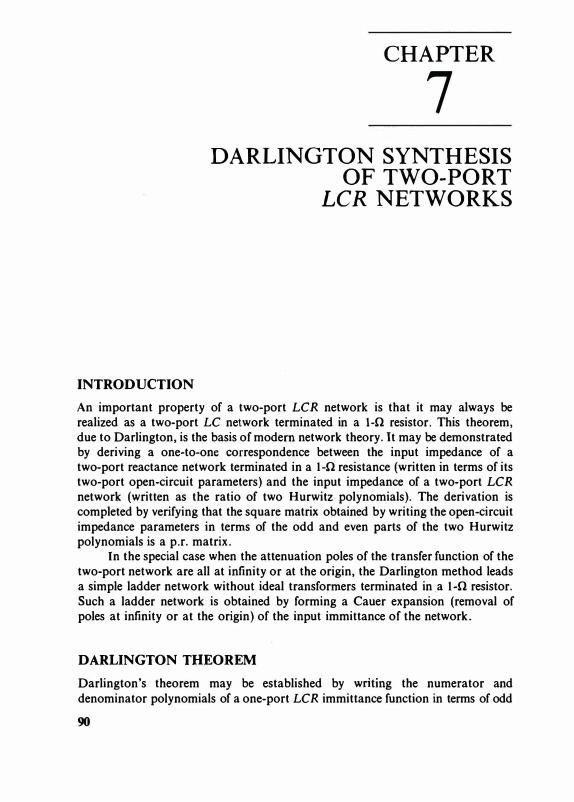
The input impedance of the two-port reactance network terminated in a l-!l resistance in Fig. 7-l in terms of the open-circuit parameters in Fig. 7-2 is
as is readily verified starting with
Z(s)
FIGURE 7-1
Reactance network
Two-port reactance network.
(7-5)
[V] = [Z][/] (7-6)
92 SYNTHESIS OF LUMPED ELEMENT, DISTRIBUTED AND PLANAR FILTERS
Z(s)
FIGURE 7-2
10
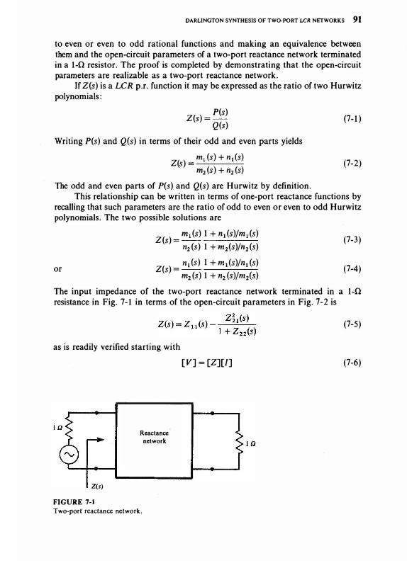
Two-port reactance network in terms of open-circuit parameters.
The immittance of the two-port reactance network may be put in the form of that in Eq. (7-3) or (7-4) by first writing it as the ratio of two polynomials:
Z(s) = Z 11 (s) + Z 11 (s)Zn(s)-Zi1 (s)
(7_7) 1 + Zn(s)
and then extracting a common term Z 11 (s) from the numerator polynomial:
Z(s) = zll (s) 1 + {[Z II (s)Z22(s)-ZL (s)]/Z II (s)}
1 + Zn(s) (7-8)
Comparing this immittance function with that in Eq. (7-3) or (7-4) indicates that a one-to-one correspondence may be possible between each situation provided the quantity in the brace in the numerator polynomial of the preceding equation can be shown to be a reactance function. This is fortunately the case since
Z 11 (s)Z22(s)-Zi 1 (s) =--
Z11(s) Yn(s) (7-9)
as is readily verified by making use of the relationship between [Z) and [ Y]:
[YJ = [Zr1
(7-10)
The input impedance of a two-port reactance network may therefore be written in terms of one-port reactance functions as
Z(s)=ZII(s) 1 + 1/Y22(s)
1 + Z22(s)
Equation (7-3) or (1-4) is consistent with Eq. (7-11) provided
Z ( )_m1(s)
II S --
nl(S)
m2(s) zll(s)=-
nl(s)
(7-11)
(7-12a)
(7-12b)
or
DARLINGTON SYNTHESIS OF TWO-PORT LCR NETWORKS 93
Z ( )-n1(s) 11 s - -
m2(s)
Z ( ) _ n2(s)
22 s --m2(s)
1 m1 (s) Yds) n1(s)
(7-12c)
(7-13a)
(7-l3b)
(7-l3c)
Writing Eq. (7-9) in terms of Eqs (7-12) or (7-13) gives
Z ( )-)m1(s)m2(s)-n1(s)n2(s) 21 s -
�-=--'------____;'----=--__.:.. n2(s) (7-14)
or (7-15)
It is now necessary to ensure that Z11 (s), Z22(s)and Z21 (s) in Eqs (7-12a), (7-12b) and (7-14) or (7-l3a), (7-l3b) and (7-15) are realizable as a two-port reactance network. This requirement is always met, providing the following two tests are met.
The quadraticforrn of the matrix Z(s) is the ratio of odd to even or even to odd Hurwitz polynomials.
Z(s) has only simple poles on the jw axis which satisfy the residue condition k� 1 > 0 , k�2 > 0 , k� 1 k�2- k�1 > 0 .
The first condition requires that Z21(s) as well as the one-port reactances Z11(s) and Z22(s) should be an odd reactance function. This condition determines whether Eq. (7-14) or (7-15) applies. To cater for the possibility that (7-14) or (7-15) may not be a perfect square, Z(s) is augmented by a Hurwitz polynomial m0(s) + n0(s):
This gives
or
Z(s) = [m1 (s)m0(s) + n1 (s)n0(s)] + [m1 (s)n0(s) + n1 (s)m0(s)][m2(s)m0(s) + n2(s)n0(s)] + [m2(s)n0(s) + n2(s)m0(s)]
Z(s) = M 1(s) + N 1(s)
· M2(s)+N2(s)
(7-16a)
(7-16b)
(7-16c)
Although Z(s) is unchanged, its odd and even parts are now different. The derivation of the open-circuit parameters of the LCR impedance function follows
94 SYNTHESIS OF LUMPED ELEMENT, DISTRIBUTED AND PLANAR FILTERS
the development leading to Eqs (7-12a), (7-12b) and (7-14). The result is
z ( s)=M1( s) (7-17) 11 N 2(s) M2( s)
Z22( s) = -- (7-18) N2( s)
() JM1( s)M2(s)-N1( s)N2( s) Z21 s = (7-19) N2( s)
The other possibility for the open-circuit parameters is readily given by N 1( s)
Z11( s)=-M2( s)
N2( s) Zds)=-
M2(s)
() JN1(s)N2(s)-M1( s)M2( s) z21 s = --'-------'=----=----M2(s)
(7-20)
(7-21)
(7-22)
The factor inside the square root sign in (7-19) is given in terms of the original variables by
M 1 ( s)M 2( s)-N 1 ( s)N 2( s) = [mMs)- n�( s) ][m1 ( s)m2( s)- n1 ( s)n2(s) ] (7-23)
Factoring the quantity m1 ( s)m2( s)-n1 (s)n2(s) into odd and even factors leads toml (s)m2(s)-nl (s)n2( s) = n ( s2- sf)"' n (s2- sf>"' (7-24)
The terms involving s i are even factors and those involving si are odd factors. To ensure that Z21 ( s) is a rational function mMs)-nMs) is set equal to the factors in Eq. (7-24) that are of odd multiplicity:
(7-25)
To ensure that m0( s) + n0( s) is a Hurwitz polynomial it is constructed by the LHP factors in (7-25):
(7-26)
This choice of m0( s) + n0(s) always guarantees a rational function for Z21(s) in Eq. (7-19). A similar statement applies to the possibility in Eq. (7-22).
The first realizability condition also requires that Z11( s), Z22(s) and Yn(s) be odd rational functions of s. Z22( s) and Y22( s) certainly meet this requirement since they are the ratios of odd to even or even to odd parts of Hurwitz polynomials M 1( s) + N 1 (s) or M 2( s) + N 2( s). However, it is not immediately obvious that this condition is met by Z11 (s) since it has not been demonstrated that M1 (s) + N2(s)
or M2(s) + N1 (s) is a Hurwitz polynomial. To establish the Hurwitz character of
DARLINGTON SYNTHESIS OF TWO-PORT LCR NETWORKS 95
these latter polynomials a new LCR impedance function Z'(s) is formed such that
Z'(s)=M1(s)+N2(s) (7-27) M2(s) + N1(s)
In order for this function to be p.r. it must satisfy conditions (2-10) and (2-11) in Chapter 2.
The first condition is met provided
is Hurwitz. M1(s)+N2(s)+M2(s)+N1(s) (7-28)
The second condition is satisfied (see Prob. 2-5 in Chapter 2 ) provided M 1 (s)M 2(s)- N 1(s)N 2(s)j,=ico � 0 (7-29)
Applying the above two tests to the original impedance Z(s) in Eq. (7-16) gives the same two relationships. Since Z(s) is known to· be p.r., Z'(s) must alsobe p.r.; M1(s)/N2(s) and N1(s)/M2(s) in Eqs (7-17) and (7-20) are therefore oddrational functions of s required.
If it can now be demonstrated that the residue condition is satisfied by Z 11 (s ), Z 22 (s) and Z 2 1 (s ), then Z (s) will be realizable as a two-port reactance networkterminated in a 1-n resistor as asserted.
It is observed that the poles of Eqs (7-17), (7-18) and (7-19) are those ofN is) or M 2(s) (with the possibility of a pole at infinity if the degree of P(s) is of degree one higher than Q(s)).
Residues may be evaluated with the help of Eqs (2-14a-c) in Chapter 2, buta more convenient formula for the present purpose (except at infinity ) is
k- P(s) I (7-30) dQ(s)/ds Q!•>=O
Employing the latter expression to calculate the residue Z 11 (s) in Eq. (7-17) yields
k11 = M 1 (s)l (7-31) N2(s) N,(s}=O
Evaluating the residues of Z22(s) and Z21(s) in Eqs (7-18) and (7-19) gives
k22 = M2(s)l N2(s) N2(s)=O
k21 = jM1(s)M2(s)l N2(s) N2(s)=O
(7-32)
(7-33)
The residue condition is therefore satisfied with the equals sign. It may also be shown that it is likewise satisfied at infinity. This completes the Darlington proof. To appreciate the notation so far consider the synthesis of the following p.r. impedance function as a two-port reactance network terminated in a 1-n resistor.
Z(s) = 2s3 + 2s2 + 2s + 12s2+2s+1
(7-34)
96 SYNTHESIS OF LUMPED ELEMENT, DISTRIBUTED AND PLANAR FILTERS
Writing this equation in the form described by Eq. (7-2) gives
Thus
( ) (2s2+ l) +(2s3+2s)
Z s= (2s2 + l) + (2s)
m1 = 2s2 + l
n1 = 2s3 + 2s
m2 = 2s2 + l
n2 =2s
The open-circuit parameters are now determined by making use of Eqs (7-l2a)
and (7-l2b):
2s2 + lZ11(s)=--
2s
2s2 + lZds)=--
2s
l z21(s)=-
2s
Z21 (s) is in this instance a perfect square and it is therefore unnecessary to augment Z(s). Furthermore, since all open-circuit parameters are odd reactance functions, the first term for this class of network is easily satisfied. It therefore only remains to satisfy the residue condition.
Forming the residues at the origin yields
k?l =t
k�2 =t
k�l =t
The residue condition is therefore met at the origin. Evaluating the residues at infinity gives
kf'l = l
ki2 = l
kit =0
The residue condition is also satisfied at infinity. Since the impedance matrix associated with Z(s) is that of a reactance network, Z(s) is realizable as a reactance network terminated in a l-0 resistor. It therefore only remains to develop an appropriate equivalent circuit for Z(s).
DARLINGTON SYNTHESIS Of TWO-PORT LCR NETWORKS 97
SYNTHESIS OF TWO-PORT LCR NETWORKS WITH ATTENUATION POLES AT INFINITY
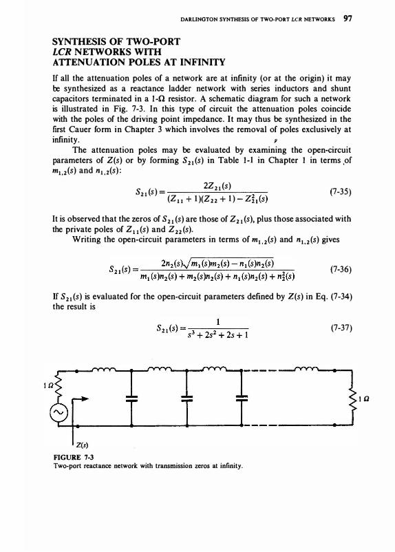
If all the attenuation poles of a network are at infinity ( or at the origin) it may be synthesized as a reactance ladder network with series inductors and shunt capacitors terminated in a 1-!l resistor. A schematic diagram for such a network is illustrated in Fig. 7-3. In this type of circuit the attenuation poles coincide with the poles of the driving point impedance. It may thus be synthesized in the first Cauer form in Chapter 3 which involves the removal of poles exclusively at infinity. p
The attenuation poles may be evaluated by examining the open-circuit parameters of Z(s) or by forming S21(s) in Table 1-1 in Chapter 1 in terms ,ofm1,2(s) and nu(s): ,
S ( )-2Z21(s)
21 s ------- ---::--(Zu + 1)(Z22 + 1)-Zi,(s) (7-35)
It is observed that the zeros of S21 (s) are those of Z21 (s), plus those associated withthe private poles of Z 11 (s) and Z22(s).
Writing the open-circuit parameters in terms of m1,2(s) and n1,2(s) gives
(7-36)
If S21(s) is evaluated for the open-circuit parameters defined by Z(s) in Eq. ( 7-34)the result is
Z(s)
FIGURE 7-3 Two-port reactance network with transmission zeros at infinity.
( 7-37)
tD
98 SYNTHESIS OF LUMPED ELEMENT, DISTRIBUTED AND PLANAR FILTERS
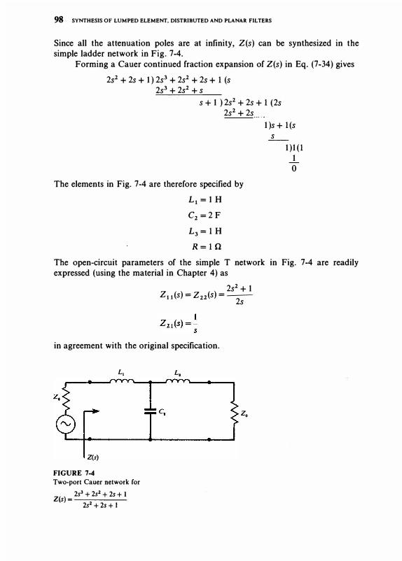
Since all the attenuation poles are at infinity, Z(s) can be synthesized in the simple ladder network in Fig. 7-4.
Forming a Cauer continued fraction expansion of Z(s) in Eq. (7-34) gives 2s2 + 2s + 1) 2s3 + 2s2 + 2s + 1 (s
2s3 + 2s2 + s s + 1 ) 2s2 + 2s + 1 (2s
2s2 + 2s
The elements in Fig. 7-4 are therefore specified by L1 = 1 HC2=2 FL3= 1 HR=1Q
1)s + 1(ss
1 )1 (1 1 0
The open-circuit parameters of the simple T network in Fig. 7-4 are readily expressed (using the material in Chapter 4) as
2s2 + 1 Z11(s)=Zu(s)=--
2s
in agreement with the original specification.
L,
Z(s) FIGURE 7-4
Two-port Cauer network for
Z(s)= 2s3+2s2+ 2s+ l 2s2+2s+l
L,
z.
DARLINGTON SYNTHESIS OF TWO-PORT LCR NETWORKS 99
DARLINGTON SYNTHESIS PROCEDURE
In the approximation problem the specification is usually stated in terms of an amplitude squared function rather than as a simple amplitude function. The first task in the synthesis problem is therefore to obtain the input driving immittance of the network from a magnitude squared transfer function. For the lossless two-port network in Fig. 7-1 between 1 fl terminations, S11 and S21 are relatedby the unitary condition in Chapter 1 by
IS 11 Uw )12 = 1 -IS 21 Uw )12 (7-38)
where w is the normal frequency variable. If IS 11 Uw )I is known it is possible to determine an appropriate value for
S11 (s) by a technique known as analytic continuation. The square of the reflection function is
(7-39)
For a rational function with real coefficients, the conjugate of a function is equal
to the function of the conjugate variable:
S!1 Uw) = Sll(jw)* (7-40)
Since the variable is imaginary, the conjugate of the variable is equal to the negative of the variable:
Thus
In terms of the variables the preceding equation becomes
IS 11 Uw )12 = Su (s)SII ( -s)l.= Jw
Combining Eqs (7-38) and (7-43) gives
S 11 (s)S11 ( -s)I•=Jw = 1 -IS21 Uw)l2
(7-41)
(7-42)
(7-43)
(7-44)
The remaining problem is to separate S 11 (s)S 11 ( -s) into its constituents. This is done by dividing the poles and zeros between the LHP and RHP.
Once S11(s) is known the input immittance of the network is given by the following standard relation:
Y(s) = _l_
-_S..:..11�(s...:.
)
1 + S11(s) (7-45)
The final step involves construction of Y(s) as a reactance ladder network. Taking S21(s) in Eq. (7-37) as an example and making use of the unitary condition
100 SYNTHESIS OF LUMPED ELEMENT, DISTRIBUTED AND PLANAR FILTERS
in Eq. (7-44) leads to s6
S 11 (s )S 11 (- s) = ---;;-----;;------;;----,--;;---(s3+2s2+2s+ 1)(-s3+2s2-2s+ 1)
and +s3S11(s)
-s3 + 2s2 + 2s + 1
Using the negative sign gives the result in Eq. (7-34):
Z(s) = 2s3 + 2s2 + 2s + 1
2s2 + 2s + l Taking the positive sign leads to
Y(s) = 2s3 + 2s2 + 2s + 1
2s2 + 2s + l The approximation problem for S21(s) is dealt with in Chapter 8.
PROBLEMS
7-1 The impedance function of a two-port LCR network is
s3 + 2s2 + 2s + 2 Z(s) = --::---:---s3 + 2s2 + 2s Synthesize this impedance function as a two-port reactance network terminated in a 1-!l resistor in
terms of its open-circuit parameters. State its transmission zeros.
7-l Obtain S21(s) for the impedance function of Prob. 7-1 and check that its zeros of transmission
agree with those obtained in Prob. 7-1. Obtain a Cauer ladder expansion of Z(s) by the removal of poles at the origin.
7-3 Show that an admittance network is always realizable as a two-port susceptance network terminated
by a 1-!l resistor [by writing Y(s) in terms of its short-circuit parameters).
7-4 The admittance of a two-port LCR network is
2s3 + 2s2 + 2s + I Y(s) = -.......,.-----2s2 + 2s +I Obtain its short-circuit parameters and determine its transmission zeros.
7-S Realize the admittance function in Prob. 7-4 as a two-port susceptance network terminated in a
1-!l resistor.
7-6 Obtain the open-circuit parameters of the following driving point impedance by augmenting it
according to (7-26):
7-7 Find H(s) and H( -s) for
7-8 Verify Eq. (7-33) using Eq. (7-30).
2s + 2 Z(s)=-s+2
INTRODUCTION
CHAPTER
10 SYNTHESIS OF
ALL-POLE LOW-PASS
ELECTRICAL
FILTERS
Electrical filters are one of the most important class of circuits used in electrical engineering. Depending on system requirement they may have low-pass, band-pass, band-stop or high-pass frequency characteristics. Modern filter theory, due to Darlington, relies on synthesis, whereby an amplitude squared transfer function specification is realized as a two-port reactance network terminated in a 1-il resistance.
The first problem in network synthesis is to construct an amplitude squared transfer function to meet the specification. This problem has been tackled in Chapter 8. The second part of network synthesis consists of finding methods whereby the corresponding network can be deduced. This chapter is mainly concerned with the latter task for filters with Butterworth or Chebyshev specifications. The conventional approach to filter theory is to develop a low-pass prototype ladder network normalized to a 1-il termination and a cutoff frequency of 1 radjs. Frequency and impedance transformations are then used to derive high-pass, band-pass and band-stop filters. This approach avoids the need to set down a multiplicity of tabulated results for the many different specifications met in practice.
141
142 SYNTHESIS OF LUMPED ELEMENT, DISTRIBUTED AND PLANAR FILTERS
Whereas the attenuation poles (transmission zeros) of Butterworth and Chebyshev low-pass amplitude squared transfer functions all lie at infinity (all-pole functons), this need not be the case in general. Inverse Chebyshev and quasi elliptic filters amplitude squared transfer functions with attenuation poles at finite frequencies are two possible examples. In the case of all-pole networks a first Cauer form extraction of the poles at infinity is all that is necessary to realize the required network. This may be understood by noting that the extraction of such poles does not impair the realizability of the remaining part of the function; nor does it affect the remaining value of its real part, since the real part contributed by such poles is identically zero. It can be shown, on the other hand, that the removal of complex poles may impair the realizability of the remainder function. The realization of networks with finite attenuation poles is separately treated in Chapter 11.
DARLINGTON SYNTHESIS PROCEDURE
In the approximation problem the specification is usually stated in terms of an amplitude squared transfer function rather than as a simple amplitude function. The first task in the synthesis problem is therefore to deduce the input driving immittance of the network from a knowledge of its magnitude squared transfer specification. For the lossless two-port network between 1-Q terminations in Fig. 10-l S 11 and S 21 are related by the unitary ·condition in Chapter l by
(10-l)
The main problem is to separate S11(s)S21( -s) into its constituents. This is done by dividing the poles and zeros between the LHP and RHP. The input immittance of the network is then given by the following standard bilinear relationship:
Z(s)
FIGURE 10-1 Doubly terminated filter circuit.
Y(s)= l-Su(s)
1+Su(s)
Reactance network
(10-2)
10
SYNTHESIS OF ALL-POLE LOW-PASS ELECTRICAL FILTERS 143
The fina\ step involves construction of Y(s) as a reactance ladder network terminated in a 1-il resistor in such a way as to realize the attenuation poles of the specification.
According to the discussion in Chapter 1, S 11 (s) is bounded real, the denominator polynomial of S 11 (s) is therefore Hurwitz, but the numerator one need not be Hurwitz. Thus, the poles of S11(s) are on the LHP and the zeros of S11(s) may have any complex plane location. The poles are therefore taken as the LHP poles of S11(s)S 11( -s), whereas the zeros are chosen in conjugate pairs from either the LHP or RHP zeros of S 11 (s)S 11 ( -s). For a minimum phase network the zeros are located on the LHP.
SYNTHESIS OF LADDER NETWORKS WITH BUTTERWORTH AMPLITUDE CHARACTERISTICS
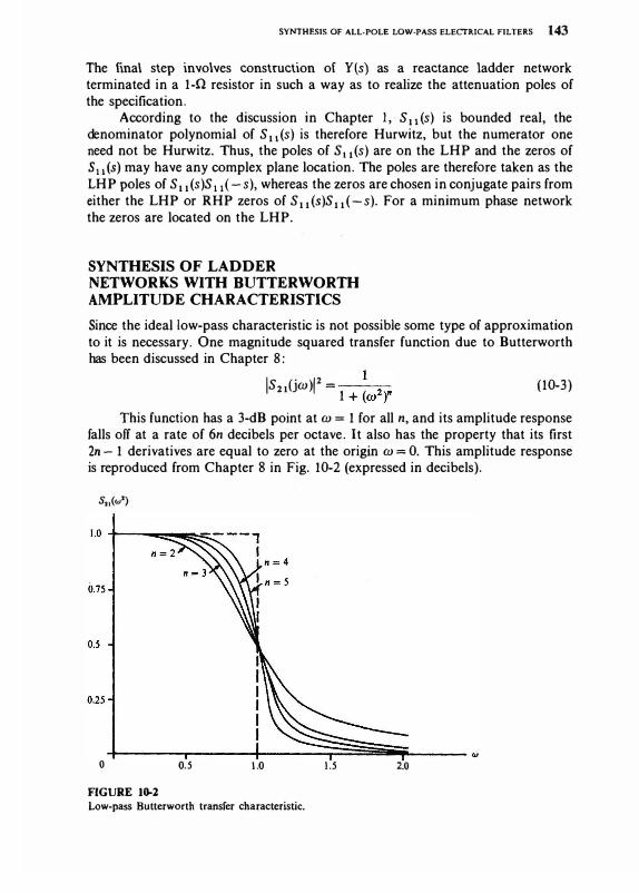
Since the ideal low-pass characteristic is not possible some type of approximation to it is necessary. One magnitude squared transfer function due to Butterworth has been discussed in Chapter 8:
IS210w)il = 1 +
:w2r
(10-3)
This function has a 3-dB point at w = 1 for all n, and its amplitude response falls off at a rate of 6n decibels per octave. It also has the property that its first 2n- 1 derivatives are equal to zero at the origin w = 0. This amplitude response is reproduced from Chapter 8 in Fig. 10-2 (expressed in decibels).
S.,(w')
0 0.5 1.0 1.5 2.0
FIGURE 10-l Low-pass Butterworth transfer characteristic.
144 SYNTHESIS OF LUMPED ELEMENT, DISTRIBUTED AND PLANAR FILTERS
Writing S11(s) in terms ofiS21Uw)l2 by replacingjw by sand having r�courseto the unitary condition yields
(_52)"S11(s)S11( -s) = 2 1+ (-s ) "
(10-4)
The poles of Eq. (10-4) are given by the roots of the denominator polynomial1 + ( -s2)" = 0 (10-Sa)
The roots of this type of polynomial may be deduced by having recourse to a root-finding subroutine. In this instance, however, the 2n roots of the preceding equation may be determined by writing Eq. (10-Sa) as
for k = 1, 2, . . . , 2n
and resorting to the following identities: - 1 = exp[j(2k-1 )n]
( - 1)" = exp[j( - nn)] The required result is
p� = exp [j( 2k +2
: - 1) n J
for k= 1, 2, . . . , 2n
for k = 1, 2, .. . , 2n
(10-Sb)
(10-Sc) (10-Sd)
(10-Se)
The roots of this polynomial reside on a unit circle in the s plane and have symmetry with respect to both the real and imaginary axis. For n odd, a pair ofroots lie on the real axis, but no roots lie on the imaginary axis for both n even or odd. The real and imaginary parts of Eq. (10-Se) are
with k = 1, 2, 3, 2n.
(2k+ n- 1 ) cr� =cos2n
n
. (2k + n - 1 ) w� = sm 2n
n
The zeros of Eq. (10-4) are the roots of the numerator polynomial
(- s2)"=0 and reside at the origin. Two possibilities are
±s"=O
(10-6a)
(10-6b)
(10-7a)
(10-7b) As an example of the construction of S 11 (s) from an amplitude squared
function consider the development of an n = 3 one with a Butterworth characteristic. The poles of the amplitude squared reflection coefficient are the roots of Eq.
(10-Sa) with n = 3:
SYNTHESIS Of ALL-POLE LOW-PASS ELECTRICAL FILTERS 145
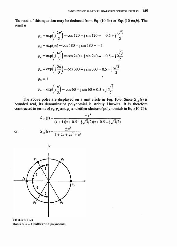
The roots of this equation may be deduced from Eq. (10-5e) or Eqs (10-6a,b). The result is
p1 = exp(j 2;) =cos 120 + j sin 120 = -0.5 + j J_} p2 = exp (jn) =cos 180 + j sin 180 = -1
p3 = exp(j �n) =cos 240 + j sin 240 = -0.5- j J_}
p4 = exp(j 5;) =cos 300 + j sin 300 = 0.5-j J_} Ps = 1
p6 = exp(j �)=cos 60 + j sin 60 = 0.5 + j {} The above poles are displayed on a unit circle in Fig. 10-3. Since S11(s) is
bounded real, its denominator polynomial is strictly Hurwitz. It is therefore constructed in terms of p1, p2 and p3 and either choice of polynomials in Eq. (10-?b):
or
FIGURE 10-3
+s3 S11 (s) = -(s + 1 )(s + 0.5 + jJ3/2)(s + 0.5-jj3/2)
+s3 S 11 (s) = ------=- ---=-1 + 2s + 2s2 + s3
jw
Roots of n =.3 Butterworth polynomial.
146 SYNTHESIS OF LUMPED ELEMENT, DISTRIBUTED AND PLANAR FILTERS
Once S 11 (s) has been deduced the input admittance of the network can be formed and the network can be synthesized by having recourse to Darlington's method. If the negative sign is used for S 11 (s) the result is
Y1.(s) 2s3 + 2s2 + 2s + 1 --= -------1 2s2 + 2s + 1
A canonical realization for Y1.(s) may now be developed by performing a Cauer-type ladder expansion of the admittance function that realizes the attenuation poles of s
21(s):
2s2 + 2s + 1 ) 2s3 + 2s2 + 2s + 1 (s -+ y 2s3 + 2s2 + s
s + 1 ) 2s2 + 2s + 1 (2s -+ y 2s2 + 2s
1)s+1(s-+y s
1) 1 (1-+ R
1
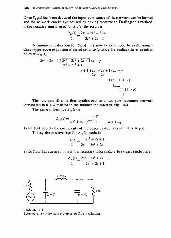
The low-pass filter is thus synthesized as a two-port reactance network terminated in a 1-0 resistor in the manner indicated in Fig. 10-4.
The general form for S 11 (s) is
+s" S11(s) =
;-a.s" + a._1s"- + · · · + a1s + a0
Table 10-1 depicts the coefficients of the denominator polynomial of S11(s). Taking the positive sign for S 11 (s) leads to
Y1.(s) 2s2 + 2s + 1
2s3 + 2s2 + 2s + 1
Since Y1.(s) has a zero at infinity it is necessary to form Z1.(s) to extract a pole there:
u,= L,
g,= c,
FIGURE 10-4
Z1.(s) 2s3 + 2s2 + 2s + 1 --=
1 2s2 + 2s + 1
10·
g,= c,
Butterworth II= 3 low-pass prototype for s,,(s) realization.
SYNTHESIS OF ALL-POLE LOW-PASS ELECTRICAL FILTERS 147
TABLE 10-1 Coefficients of Butterworth polynomials
a(s) = a0 + a1s + a2s2 +-- · + a,._1s"-1 + a,.s"
• a. a, a, a, a. a, a. a, a. a. a,.
L4I4 21 2.00000 2.00000 2.613 13 3.414 21 2.613 13 I
3.23607 5.23607 5.23607 3.23607 I 3.863 79 7.461 62 9.141 62 7.46410 3.863 70 4.493 96 10.097 84 14.591 79 14.591 79 10.097 84 4.493 96 5.12583 13.13707 21.846 15 25.688 36 21.84615 13.13707 5.125 83 5.758 77 16.58172 31.16344 41.986 39 41.986 39 31.163 44 16.581 72 5.758 77
10 6.39245 20.431 73 42.802 06 64.88240 74.233 43 64.882 40 42.80206 20.431 73 6.39245 I
Source: Matthaei, G. L., Young, L. and Jones, E. M. T., Microwave Filters, Impedance-matching Networks and
Coupling Structures, Artech House, Norwood, MA, 1980 ..
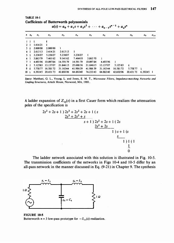
A ladder expansion of Zin(s) in a first Cauer form which realizes the attenuationpoles of the specification is
2s2 + 2s + 1 ) 2s3 + 2s2 + 2s + 1 ( s 2s3 + 2s2 + s
s + 1 ) 2s2 +2s + 1( 2s 2s2 + 2s
1 ) s + 1 (s s
1 ) 1 ( 1 1 0
The ladder network associated with this solution is illustrated in Fig. 10-5. The transmission coefficients of the networks in Figs 10-4 and 10-5 differ by an all-pass network in the manner discussed in Eq. (9- 21) in Chapter 9. The synthesis
g, = L,
I.Q g, = c,
FIGURE 10-5
Butterworth n = 3 low-pass prototype for -S11(s) realization.
148 SYNTHESIS Of LUMPED ELEMENT, DISTRIBUTED AND PLANAR FILTERS
y, u •
(a)
(b)
.-----'I"VY'Y'"'o�--r---''VY'Y"\------------rrv-Y"\. --r----.
��..____--&.--!··
g, u.
(c)
g • .----..Jf"VY'Y'"'o'--...--f"YYV"\----------...-...rYYT>-----,
I� !·• -----�-------------'
(d)
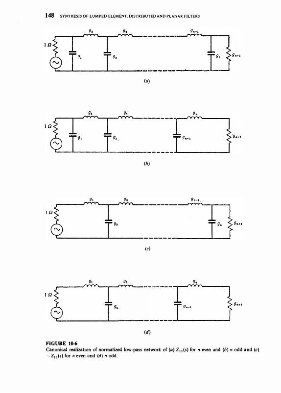
FIGURE 1�
u ...
Canonical realization of normalized low-pass network of (a) S 11 (s) for n even and (b) n odd and (c) -S11(s) for n even and (d) n odd.
SYNTHESIS OF ALL-POLE LOW-PASS ELECTRICAL FILTERS 149
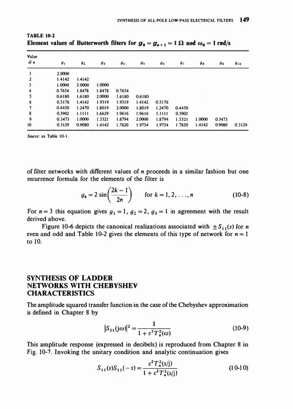
TABLE 10-2
Element values of Butterworth filters for Yo = g,. + 1 = 1 n and Wo = 1 radfs
Value
of n g, g, g, g. g, e. g, g, g.
2.0000
2 1.4142 1.4142
3 1.0000 2.0000 1.0000
4 0.7654 1.8478 1.8478 0.7654
0.6180 1.6180 2.0000 1.6180 0.6180
0.5176 1.4142 1.9319 1.9319 1.4142 0.5176
7 0.4450 1.2470 1.8019 2.0000 1.8019 1.2470 0.4450
8 0.3902 1.1111 1.6629 1.9616 1.9616 1.1111 0.3902
9 0.3473 1.0000 1.5321 1.8794 2.0000 1.8794 1.5321 1.0000 0.3473
10 0.3129 0.9080 1.4142 1.7820 1.9754 1.9754 1.7820 1.4142 0.9080
Source: as Table 10-1.
g,.
0.3129
of filter networks with different values of n proceeds in a similar fashion but one recurrence formula for the elements of the filter is
(2k -1) 9•=2sin � for k=1,2, ... ,n (10-8)
For n = 3 this equation gives 91 = 1, 92 = 2, 93 = 1 in agreement with the result derived above.
Figure 10-6 depicts the canonical realizations associated with ± S 11 (s) for n
even and odd and Table 10-2 gives the elements of this type of network for n = 1 to 10.
SYNTHESIS OF LADDER NETWORKS WITH CHEBYSHEV CHARACTERISTICS
The amplitude squared transfer function in the case of the Chebyshev approximation is defined in Chapter 8 by
IS2tUw)i2 = 1 + t:}T;(w) (10-9)
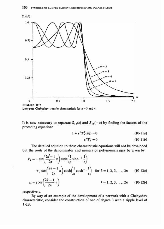
This amplitude response (expressed in decibels) is reproduced from Chapter 8 in Fig. 10-7. Invoking the unitary condition and analytic continuation gives
t:2T;(s/j) S11(s)S11(-s)=1+t:2T;(sfj) (10-10)
}50 SYNTHESIS OF LUMPED ELEMENT, DISTRIBUTED AND PLANAR FILTERS
S11(w')
1.0
0.75
0.5.
0.25
0 FIGURE 10-7
0.5 ).0
Low-pass Chebyshev transfer characteristic for n = 3 and 4.
1.5 w
2.0
It is now necessary to separate S11 (s) and S 11 ( - s) by finding the factors of the preceding equation:
1 + e2T;(sjj) = 0
e2T; = 0
(l0-11a)
(10-llb)
The detailed solution to these characteristic equations will not be developed but the roots of the denominator and numerator polynomials may be given by
. 21( - 1 . l . _ I l ( d ) ( ) Pk = -sm � n smh � smh ;
. (2k-l ) ( • •) + J cos � n cosh � cosh-
1 ;
(2k-1 ) zk= j cos � n
respectively.
for k = l, 2, 3, ... , 2n (l0-l2a)
k = 1, 2, 3, . . . , 2n (10-12b)
By way of an example of the development of a network with a Chebyshev characteristic, consider the construction of one of degree 3 with a ripple level of 1 dB.
SYNTHESIS OF ALL-POLE LOW-PASS ELECTRICAL FILTERS 151
The required poles are given by the roots of Eq. (10-lla) or (10-12a) as
. n . h( 1 . h I 1) . n h(1 . h I
1)p 1 = - sm -sm -sm - - + J cos -cos -sm - -6 3 e 6 3 e
. 3n . h(1 . h 1 1) . 3n h(1 . h 1 1) p2 = -sm - sm - sm - - + J cos -cos -sm - -
6 3 e 6 3 e
. 5n . h(1 . h 1 1) . 5n h(1 . h 1
1)p3= -sm-sm -sm - - +Jcos-cos -sm - -6 3 e 6 3 e
. 7n . h(1 . h 1 1) . 7n h(1 . h 1 1) p4=-sm-sm -sm - - +Jcos-cos -sm - -
6 3 e 6 3 e
. 9n . h(1 . h 1 1) . 9n h(1 . h 1 1)Ps = -sm-sm - sm - - + J cos-cos -sm - -
6 3 e 6 3 e
. lln . h(1 . h
_1 1) . lln h(1 . _1 1)p6 = - sm - sm - sm - + J cos - cos -smh -6 3 e 6 3 e
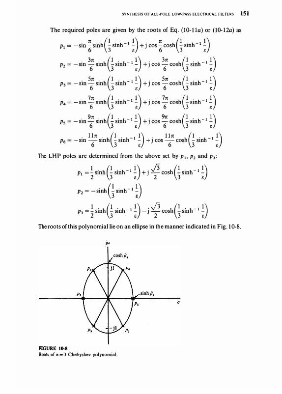
The LHP poles are determined from the above set by p1, p2 and p3:
1 . h(1 . h- 11) ._fi h(1 .
-11)p1 =-sm -sm - + J -cos - smh -
2 3 e 2 3 e
p2 = -sinhG sinh-1 D
1 . h(1 . h 1 1) . fi h(1 . h 1 1)p3 = -sm -sm - - -J - cos - sm - -2 3 e 2 3 e
The roots of this polynomial lie on an ellipse in the manner indicated in Fig. 10-8.
jw
sinhp.
FIGURE 10-8 Roots of n = 3 Chebyshev polynomial.
152 SYNTHESIS OF LUMPED ELEMENT, OJSTRIBliTED AND PLANAR FILTERS
For a 1-dB ripple level e is fixed as
E = 0.509
and p1, p2 and p3
are given by
p1 = -0.494 1 7
P2 = - 0.247 08 + j0.965 99
p3
= - 0.247 08 - j0.965 99
The denominator polynomial of S u (s) is therefore described by
s3 + 0.988 34s2 + 1 .238 41s + 0.491 3 1
Table 10-3 summarizes the coefficients o f this polynomial for n = 1 t o 10 for ripple levels oft, 1 and 2 dB. The numerator polynomial P(s) may be directly constructed from either the LHP or RHP roots of Eq. (10-llb).
± T3(s/j) = 0
The roots of the preceding equation may be evaluated by Eq. ( 10- 1 2b) or by having recourse to the recurrence form for T"(w) in Chapter 8. Making use of the latter relationship with e = 0.509 leads to
P(s) = ±0.509(4s3 + 3s)
The required form for S u (s) is therefore
S 11 (s) = P(s)
= ±0.509(4s3 + 3s)a
Q(s) s3 + 0.988 34s2 + 1 .2384s + 0.491 31
The multiplication constant a is introduced to ensure that S u (s) is bounded real (unity) at s = joo. The required result is
S ± (s3 + 0.75s)
1 1 (s) = s3 + 0.988 34s2 + 1 .2384s + 0.49 1 3 1
Taking the negative sign yields the input admittance of the network as
Yin(s) 2s3 + 0.988 34s2 + 1 .988 41s + 0.491 31
0.988 34s2 + 0.488 41s + 0.491 31
Forming a Cauer ladder network by removal of poles a t infinity which realizes the attenuation poles of s
21 (s) gives
c1 =2.024F
L2 = 0.994 H
c3
= 2.024 F
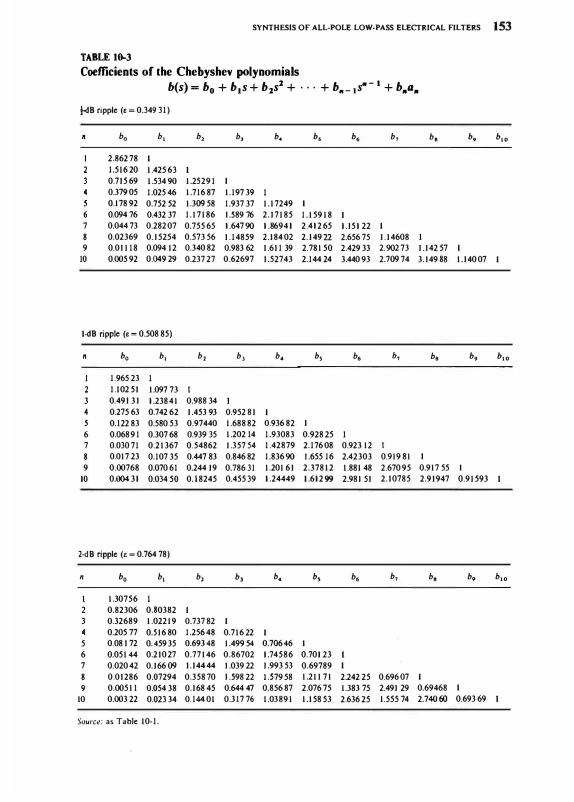
TABLE 10-3
SYNTHESIS OF ALL-POLE LOW-PASS ELECfRICAL FILTERS 153
Coefficients of the Chebyshev polynomials
b(s) = b0 + b1s + b2s2 + --- + b,_1s"-1 + b,.a,.
j.<lB ripple (e = 0.349 31)
bo b, b, b, b. b, b. b, b. b. b,o
2.862 78 I
1.516 20 1.425 63 I
0.715 69 1.534 90 1.25291 I
0.379 05 1.025 46 1.716 87 1.197 39 I
0.178 92 0.752 52 1.309 58 1.937 37 1.17249 I
6 0.094 76 0.432 37 1.17186 l.S89 76 2.17185 1.159 18 I
7 0.044 73 0.282 07 0.755 65 1.64790 1.86941 2.412 65 1.151 22 I
8 0.02369 0.15254 0.573 56 1.14859 2.184 02 2.149 22 2.656 75 1.14608
9 0.01118 0.094 12 0.340 82 0.983 62 1.611 39 2.781 50 2.429 33 2.902 73 1.142 57 I
10 0.005 92 0.049 29 0.237 27 0.62697 1.52743 2.144 24 3.440 93 2.70974 3.149 88 1.140 07 I
I -dB ripple (e = 0.508 85)
bo b, b, b, b, b, b. b, bo b. b,o
1.965 23 I
1.102 51 1.097 73 I
0.491 31 1.23841 0.988 34
0.275 63 0.742 62 1.453 93 0.952 81 I
0.122 83 0.580 53 0.97440 1.688 82 0.936 82 I
6 0.068 91 0.307 68 0.939 35 1.202 14 1.93083 0.928 25 I
7 O.oJO 71 0.21367 0.54862 1.357 54 1.42879 2.176 08 0.923 12 I
8 0.017 23 0.107 35 0.447 83 0.846 82 1.83690 1.655 16 2.42303 0.919 81
9 0.00768 0.070 61 0.244 19 0.78631 1.201 61 2.37812 1.881 48 2.670 95 0.917 55 I
10 0.00431 0.034 50 0.18245 0.455 39 1.24449 1.61299 2.981 51 2.10785 2.91947 0.91593 I
2-dB ripple (e = 0.764 78)
n bo b, b, b, b, b, b. b, bo b. b,o
1.30756 I
0.82306 0.80382 I
0.32689 1.02219 0.737 82 I
0.205 77 0.516 80 1.256 48 0.716 22 I
5 0.081 72 0.459 35 0.69348 1.499 54 0.70646 I
6 0.05144 0.210 27 0.77146 0.86702 1.74586 0.701 23
7 0.020 42 0.166 09 1.144 44 1.039 22 1.993 53 0.69789 I
8 0.01286 0.07294 0.358 70 l.S98 22 l.S79 58 1.211 71 2.242 25 0.696 07 I
9 0.00511 0.054 38 0.168 45 0.644 47 0.856 87 2.076 75 1.383 75 2.491 29 0.69468 I
10 0.003 22 0.023 34 0.14401 0.317 76 1.03891 1.158 53 2.636 25 1.555 74 2.74060 0.693 69 I
Source: as Table 10-1.
154 SYNTHESIS OF LUMPED ELEMENT, D!STlUBUTED AND PLANAR FILTERS
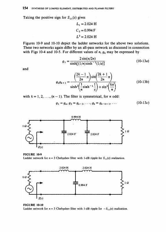
Taking the positive sign for S11(s) gives
L1 =2.024 H
C2 =0.994F
L3 = 2.024 H
Figures 10-9 and 10-10 depict the ladder networks for the above two solutions. These two networks again differ by an all-pass network as discussed in connection with Figs 10-4 and 10-5. For different values of n, gk may be expressed by
and
2 sin(n/2n) Or= sinh[(1/n)sinh-1(1/e)]
(2k - 1 ) . (2k+1 ) -- n sm --n 2n 2n
with k = 1, 2, ... , (n -1). The filter is symmetrical, for n odd:
9! =g., 02 = 0•-l• · · . , 9t = 0•-k+ I• • • •
.0.994 H
2.024 F 2.024 F
Z(s)
FIGURE 10-9
10
Ladder network for n = 3 Chebyshev filter with 1-dB ripple for S,,(s) realization.
2.024 H 2.024 H
10 0.994 F
Z(s)
FIGURE 10-10 Ladder network for n = 3 Chebyshev filter with 1-dB ripple for -S11(s) realization.
(10-13a)
(l0-13b)
(10-13c)
SYNTHESIS OF ALL-POLE LOW-PASS ELECTRICAL FILTERS 155
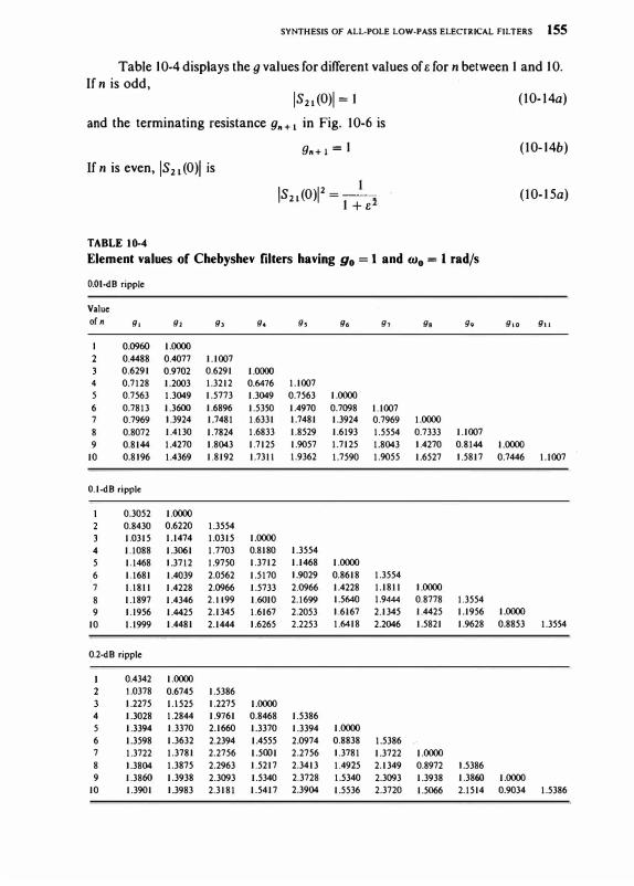
Table l 0-4 displays the g values for different values of e for n between l and l 0. If n is odd,
IS2I(O)I=l (10-14a) and the terminating resistance g.+ 1 in Fig. 10-6 is
9n+ I= l (10-l4b) lfn is even, IS21(0)I is
IS21 (0)12 = -1-2 l+s
(10-l5a)
TABLE 10-4
Element values of Chebyshev filters having g0 = 1 and w0 = 1 radfs
O.QI-dB ripple
Value of n g, g, g, g. g, g. g, g• 99 g,. gil
0.0960 1.0000
0.4488 0.4077 1.1007 0.6291 0.9702 0.6291 1.0000
4 0.7128 1.2003 1.3212 0.6476 1.1007
5 0.7563 1.3049 1.5773 1.3049 0.7563 1.0000
6 0.7813 1.3600 1.6896 1.5350 1.4970 0.7098 l.l007 7 0.7969 1.3924 1.7481 1.6331 1.7481 1.3924 0.7969 1.0000
8 0.8072 1.4130 1.7824 1.6833 1.8529 1.6193 1.5554 0.7333 1.1007
9 0.8144 1.4270 1.8043 1.7125 1.9057 1.7125 1.8043 1.4270 0.8144 1.0000
10 0.8196 1.4369 1.8192 1.73ll 1.9362 1.7590 1.9055 1.6527 1.5817 0.7446 l.l007
0.1-dB ripple
0.3052 1.0000
0.8430 0.6220 1.3554
1.0315 l.l474 1.0315 1.0000
4 1.1088 1.3061 1.7703 0.8180 1.3554
5 1.1468 1.3712 1.9750 1.3712 1.1468 1.0000
6 1.1681 1.4039 2.0562 1.5170 1.9029 0.8618 1.3554
7 l.l8ll 1.4228 2.0966 1.5733 2.0966 1.4228 1.18ll 1.0000
8 1.1897 1.4346 2.ll99 1.6010 2.1699 1.5640 1.9444 0.8778 1.3554
9 l.l956 1.4425 2.1345 1.6167 2.2053 1.6167 2.1345 1.4425 1.1956 1.0000
10 l.l999 1.4481 2.1444 1.6265 2.2253 1.6418 2.2046 1.5821 1.9628 0.8853 1.3554
0.2-d 8 ripple
0.4342 1.0000
1.0378 0.6745 1.5386
1.2275 l.l525 1.2275 1.0000
4 1.3028 1.2844 1.9761 0.8468 1.5386
5 1.3394 1.3370 2.1660 1.3370 1.3394 1.0000
6 1.3598 1.3632 2.2394 1.4555 2.0974 0.8838 1.5386
7 1.3722 1.3781 2.2756 1.5001 2.2756 1.3781 1.3722 1.0000
8 1.3804 1.3875 2.2963 1.5217 2.3413 1.4925 2.1349 0.8972 1.5386
9 1.3860 1.3938 2.3093 1.5340 2.3728 1.5340 2.3093 1.3938 1.3860 1.0000
10 1.3901 1.3983 2.3181 1.5417 2.3904 1.5536 2.3720 1.5066 2.1514 0.9034 1.5386
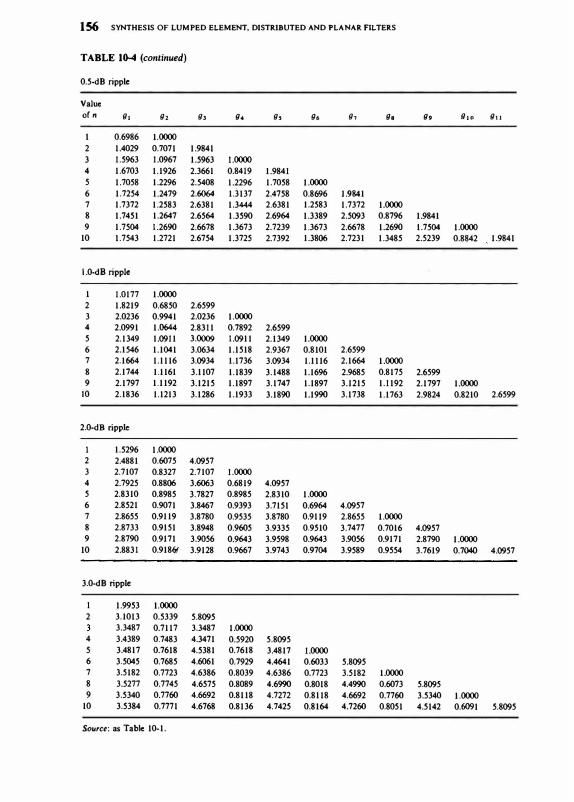
156 SYNTHESIS OF LUMPED ELEMENT, DISTRIBUTED AND PLANAR FILTERS
TABLE 10-4 (continued)
0.5-dB ripple
Value of n g, gz g, g. g, g. g, g. g. g,o g"
I 0.6986 1.0000
2 1.4029 0.7071 1.9841
3 1.5963 1.0967 1.5963 1.0000
4 1.6703 1.1926 2.3661 0.8419 1.9841 5 1.7058 1.2296 2.5408 1.2296 1.7058 1.0000
6 1.7254 1.2479 2.6064 1.3137 2.4758 0.8696 1.9841 7 1.7372 1.2583 2.6381 1.3444 2.6381 1.2583 1.7372 1.0000 8 1.7451 1.2647 2.6564 1.3590 2.6964 1.3389 2.5093 0.8796 1.9841 9 1.7504 1.2690 2.6678 1.3673 2.7239 1.3673 2.6678 1.2690 1.7504 1.0000
10 1.7543 1.2721 2.6754 1.3725 2.7392 1.3806 2.7231 1.3485 2.5239 0.8842 1.9841
1.0-dB ripple
1.0177 1.0000 2 1.8219 0.6850 2.6599
3 2.0236 0.9941 2.0236 1.0000 4 2.0991 1.0644 2.8311 0.7892 2.6599 5 2.1349 1.0911 3.0009 1.0911 2.1349 1.0000 6 2.1546 1.1041 3.0634 1.1518 2.9367 0.8101 2.6599 7 2.1664 1.1116 3.0934 1.1736 3.0934 1.1116 2.1664 1.0000 8 2.1744 1.1161 3.1107 1.1839 3.1488 1.1696 2.9685 0.8175 2.6599 9 2.1797 1.1192 3.1215 1.1897 3.1747 1.1897 3.1215 1.1192 2.1797 1.0000
10 2.1836 1.1213 3.1286 1.1933 3.1890 1.1990 3.1738 1.1763 2.9824 0.8210 2.6599
2.0-dB ripple
1.5296 1.0000 2 2.4881 0.6075 4.0957 3 2.7107 0.8327 2.7107 1.0000 4 2.7925 0.8806 3.6063 0.6819 4.0957 5 2.8310 0.8985 3.7827 0.8985 2.8310 1.0000 6 2.8521 0.9071 3.8467 0.9393 3.7151 0.6964 4.0957
7 2.8655 0.9119 3.8780 0.9535 3.8780 0.9119 2.8655 1.0000 8 2.8733 0.9151 3.8948 0.9605 3.9335 0.9510 3.7477 0.7016 4.0957 9 2.8790 0.9171 3.9056 0.9643 3.9598 0.9643 3.9056 0.9171 2.8790 1.0000
10 2.8831 0.91861 3.9128 0.9667 3.9743 0.9704 3.9589 0.9554 3.7619 0.7040 4.0957
3.0-dB ripple
1.9953 1.0000
2 3.1013 0.5339 5.8095 3.3487 0.7117 3.3487 1.0000
4 3.4389 0.7483 4.3471 0.5920 5.8095 5 3.4817 0.7618 4.5381 0.7618 3.4817 1.0000 6 3.5045 0.7685 4.6061 0.7929 4.4641 0.6033 5.8095 7 3.5182 0.7723 4.6386 0.8039 4.6386 0.7723 3.5182 1.0000 8 3.5277 0.7745 4.6575 0.8089 4.6990 0.8018 4.4990 0.6073 5.8095 9 3.5340 0.7760 4.6692 0.8118 4.7272 0.8118 4.6692 0.7760 3.5340 1.0000
10 3.5384 0.7771 4.6768 0.8136 4.7425 0.8164 4.7260 0.8051 4.5142 0.6091 5.8095
Source: as Table 10-1.
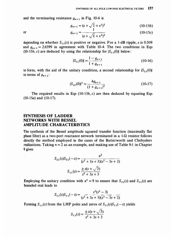
SYNTHESIS OF ALL-POLE LOW-PASS ELECTRICAL FILTERS 157
and the terminating resistance 9n + 1 in Fig. 10-6 is
9n+ I = (e + .J1 + e2)21
or 9n + I = ---=--(e +
.J1 + e2)2
( 10- 1 5b)
( 10- 1 5c)
depending on whether S1 1 (s) is positive or negative. For a 1-dB ripple, e is 0.509 and 9n + 1 = 2.6599 in agreement with Table 10-4. The two conditions in Eqs (10- 15b, c) are deduced by using the relationship for IS1 1 (0)1 below :
IS1 1 (0)1 =1 - g•+ l (10- 16) 1 + 9n + I
to form, with the aid of the unitary condition, a second relationship for IS2
1 (0)1 · in terms of g.+ 1 :
ISzi (O)Jl = 4g•
+ l( l + g. + d2
(10-17)
The required results in Eqs ( 10- 1 5b, c) are then deduced by equating Eqs (10-15a) and (10- 1 7).
SYNTHESIS OF LADDER NETWORKS WITH BESSEL AMPLITUDE CHARACTERISTICS
The synthesis of the Bessel amplitude squared transfer function (maximally flat phase filter) as a two-port reactance network terminated in a 1-Q resistor follows directly the method employed in the cases of the Butterworth and Chebyshev realizations. Taking n = 2 as an example, and making use of Table 9-1 in Chapter 9 gives
cx2 S (s)S ( - s) =
--,--------21 2 1
(s2 + 3s + 3)(s2 - 3s + 3)
S (s) = ± s(s + j3)
1 1 s2 + 3s + 3
Employing the unitary condition with cx2 = 9 to ensure that S 2
1 (s) and S 1 1 (s) are bounded real leads to
s2(s2 - 3) Su(s)Su ( - s) =
(s2 + 3s + 3)(s2 - 3s + 3)
Forming S1 1 (s) from the LHP poles and zeros of S1 1 (s)S1 1 ( - s) yields
S (s) = ± s(s + j3)
1 1 s2 + 3s + 3
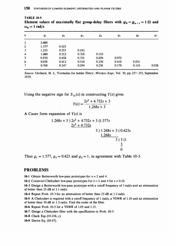
158 SYNTHESIS O F LUMPED ELEMENT, DISTRIBUTED AND PLANAR FILTERS
TABLE 10-5 Element values of maximally flat group-delay filters with g0 = 9. + 1 = 1 0 and w0 = 1 rad/s
n 9t 9> 93 94 9s 96 97
2.000 2 1 .577 0.423 3 1 .255 0.553 0.192 4 1 .060 0.512 0.318 0.1 10 5 0.930 0.458 0.331 0.209 0.072 6 0.838 0.41 2 0.3 16 0.236 0.418 0.051 7 0.768 0.347 0.294 0.238 0.178 0.110 0.038
Source: Orchard, H. J., 'Formulas for ladder filters', Wireless En9r, Vol. 30, pp. 257-353, September 1939.
Using the negative sign for S 11 (s) in constructing Y(s) gives
( ) 2s2 + 4.732s + 3
Y s
= ------
1 .268s + 3
A Cauer form expansion of Y(s) is
1 .268s + 3 ) 2s2 + 4.732s + 3 (1 .577s 2s2 + 4.732s
3 ) l .268s + 3 ( 0.423s 1 .268s
3 ) 3 (1 3
0
Thus g1 = 1 .577, g2 = 0.423 and g3 = l , in agreement with Table 10-5.
PROBLEMS
10-1 Obtain Butterworth low-pass prototypes for n = 2 and 4.
10-2 Construct Chebyshev low-pass prototypes for n = 2 and 4 for e = 0.10.
10-3 Design a Butterworth low-pass prototype with a cutoff frequency of l rad/s and an attenuation of better than 25 dB at 1 . l radfs .
10-4 Repeat Pro b. 10-3 for an attenuation of better than 25 dB at 1 .2 rad/s .
10-5 A Chebyshev is required with a cutoff frequency of I rad/s, a VSWR of 1 . 10 and an attenuation of better than 30 dB at 1 .3 radfs. Find the order of the filter.
10-6 Repeat Prob. 10-5 for a VSWR of 1 .05 and 1 . 15 .
10-7 Design a Chebyshev filter with the specification in Prob. 10-5. 10-8 Check Eqs (10-l5b, c). 10-9 Derive Eq. (10-17).

SYNTHESIS OF ALL-POLE LOW-PASS ELECTRICAL FILTERS 159
1�10 Using Eqs (1�1 3a, b) verify that Chebyshev filters are symmetrical provided n is odd.
1�11 Verify that Butterworth filters are symmetrical for n odd and even.
1�12 Verify that Eq. (1�8) is consistent with Table 1�1.
1�13 Verify that Eqs (10-l3a, b) are consistent with Table 10-4 for ripple levels oft = f, 1 and 1! dB.
1�14 By dividing the real parts of Eq. (l� 12a) by cosh[(1/n) sinh - 1 ( l/t)] and the imaginary parts by sinh[(1/n) sinh - 1(1/t)] show that the poles of S 1 1 (s) lie on an ellipse.
BIBLIOGRAPHY
Matthaei, G. L, Young, L. and Jones, E. M. T. Microwave Filters, Impedance-matching Ne.tworks and Coupling Structures, Artech House, Norwood, MA, 1980.
Orchard, H. J., 'Formulas for ladder filters', Wireless Engr, Vol. 30, pp. 257-353, September, 1939.

![5 Design of RF and Microwave Filters [호환 모드]home.sogang.ac.kr/sites/eemic/lecture/note02/Lists... · PTPSP PPSP 2 21 2 2 11 2 == =G= () 1 1 1 2w w D N P P P tran in LR =+-G](https://img.pdfslide.net/doc/110x75/5d44a92388c9936c128deddf/5-design-of-rf-and-microwave-filters-home-ptpsp-ppsp-2-21-2.jpg)