Embed Size (px)
Citation preview
Chapter 8
Hypothesis Testing with Two Samples
1Larson/Farber 4th ed
Chapter Outline
• 8.1 Testing the Difference Between Means (Large Independent Samples)
• 8.2 Testing the Difference Between Means (Small Independent Samples)
• 8.3 Testing the Difference Between Means (Dependent Samples)
• 8.4 Testing the Difference Between Proportions
2Larson/Farber 4th ed
Section 8.1
Testing the Difference Between Means (Large Independent Samples)
3Larson/Farber 4th ed
Section 8.1 Objectives
• Determine whether two samples are independent or dependent
• Perform a two-sample z-test for the difference between two means μ1 and μ2 using large independent samples
4Larson/Farber 4th ed
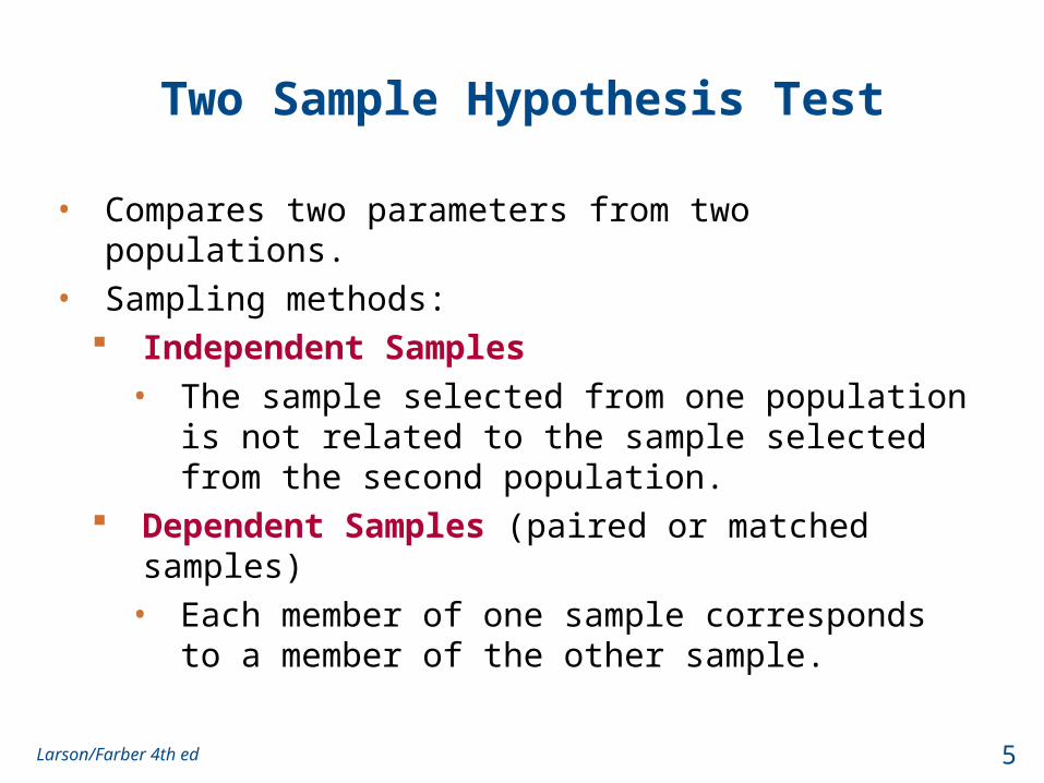
Two Sample Hypothesis Test
• Compares two parameters from two populations.
• Sampling methods: Independent Samples
• The sample selected from one population is not related to the sample selected from the second population.
Dependent Samples (paired or matched samples)
• Each member of one sample corresponds to a member of the other sample.
5Larson/Farber 4th ed
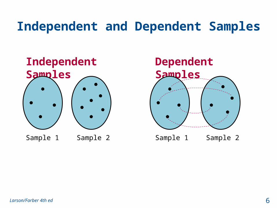
Independent and Dependent Samples
Independent Samples
Sample 1 Sample 2
Dependent Samples
Sample 1 Sample 2
6Larson/Farber 4th ed
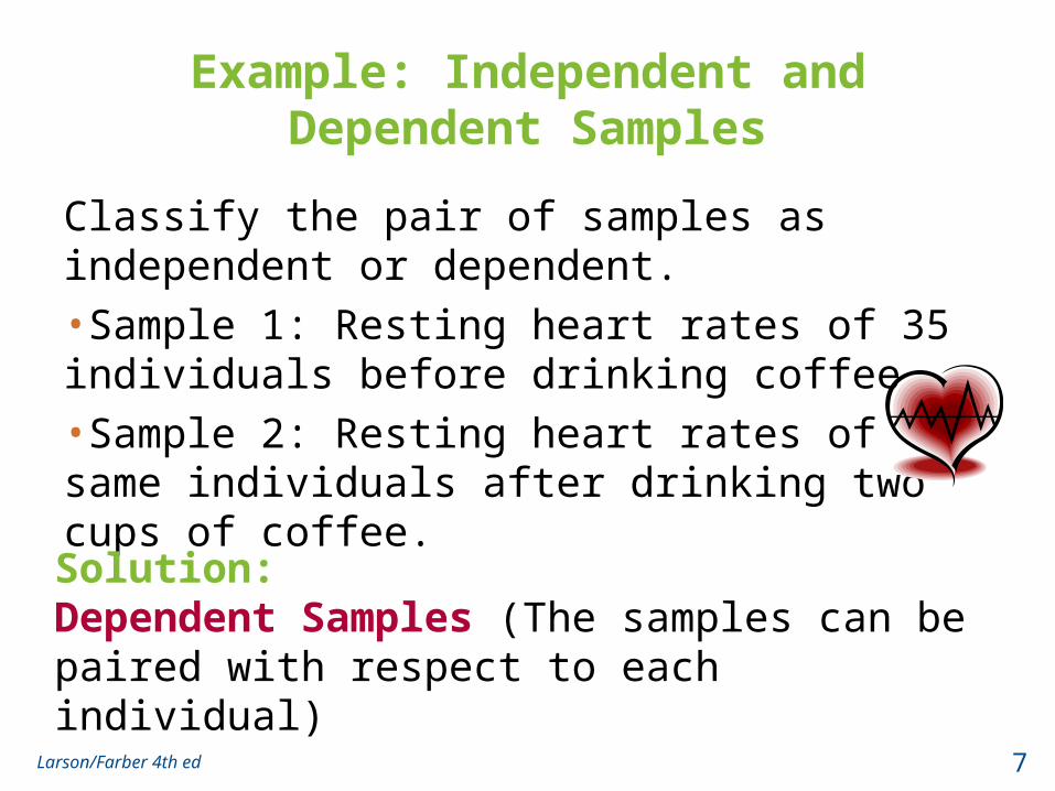
Example: Independent and Dependent Samples
Classify the pair of samples as independent or dependent.
•Sample 1: Resting heart rates of 35 individuals before drinking coffee.
•Sample 2: Resting heart rates of the same individuals after drinking two cups of coffee.
Solution:Dependent Samples (The samples can be paired with respect to each individual)
7Larson/Farber 4th ed
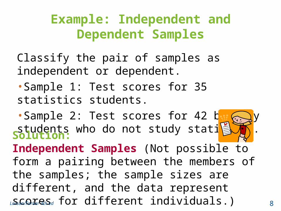
Example: Independent and Dependent Samples
Classify the pair of samples as independent or dependent.
•Sample 1: Test scores for 35 statistics students.
•Sample 2: Test scores for 42 biology students who do not study statistics.
Solution:Independent Samples (Not possible to form a pairing between the members of the samples; the sample sizes are different, and the data represent scores for different individuals.)
8Larson/Farber 4th ed
Two Sample Hypothesis Test with Independent Samples
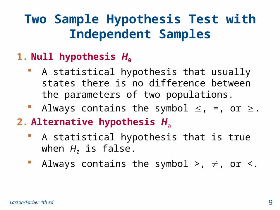
1. Null hypothesis H0
A statistical hypothesis that usually states there is no difference between the parameters of two populations.
Always contains the symbol , =, or .
2. Alternative hypothesis Ha
A statistical hypothesis that is true when H0 is false.
Always contains the symbol >, , or <.
9Larson/Farber 4th ed
Two Sample Hypothesis Test with Independent Samples
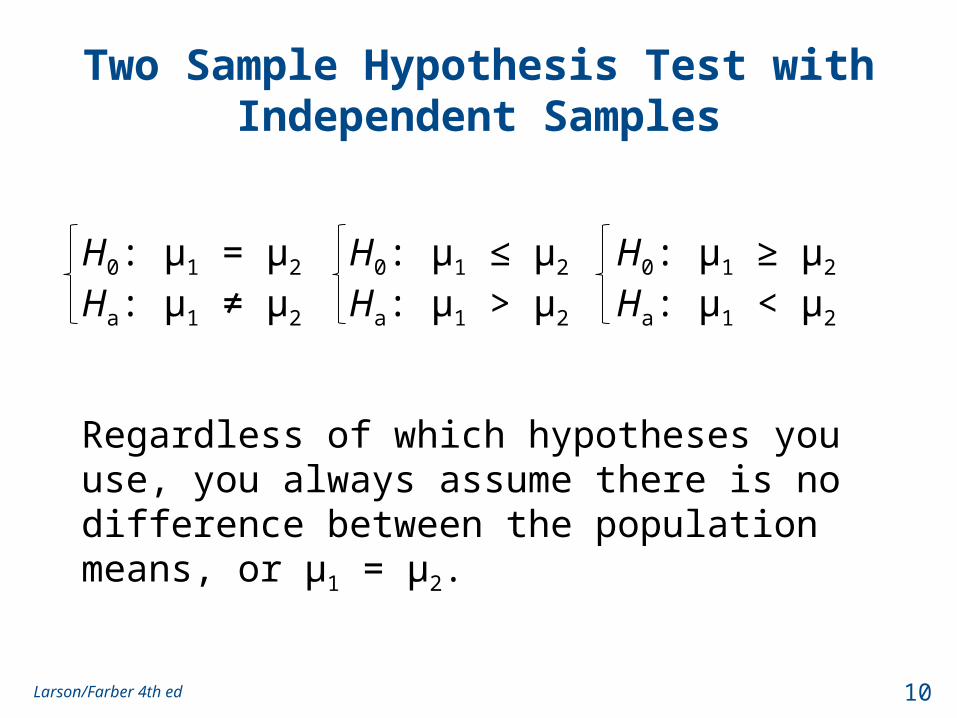
H0: μ1 = μ2
Ha: μ1 ≠ μ2 H0: μ1 ≤ μ2
Ha: μ1 > μ2 H0: μ1 ≥ μ2
Ha: μ1 < μ2
Regardless of which hypotheses you use, you always assume there is no difference between the population means, or μ1 = μ2.
10Larson/Farber 4th ed
Two Sample z-Test for the Difference Between Means
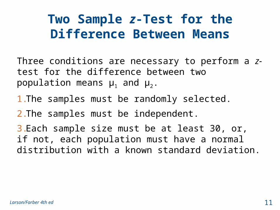
Three conditions are necessary to perform a z-test for the difference between two population means μ1 and μ2.
1.The samples must be randomly selected.
2.The samples must be independent.
3.Each sample size must be at least 30, or, if not, each population must have a normal distribution with a known standard deviation.
11Larson/Farber 4th ed
Two Sample z-Test for the Difference Between Means
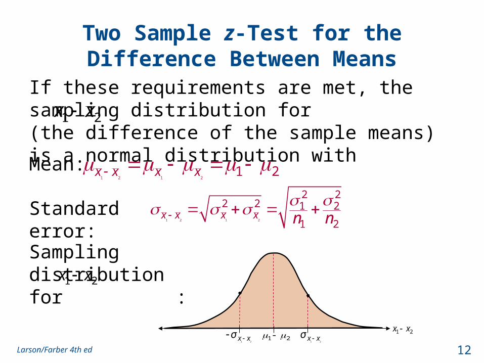
If these requirements are met, the sampling distribution for (the difference of the sample means) is a normal distribution with
1 2 1 21 2x x x x
1 2x x
1 2 1 2
2 22 2 1 2
1 2x x x x n n
Sampling distribution for :
1 2x x
Mean:
Standard error:
1 2x x1 2
1 2x xσ
1 2x xσ
12Larson/Farber 4th ed
Two Sample z-Test for the Difference Between Means
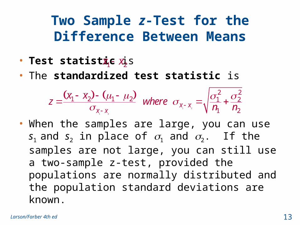
• Test statistic is
• The standardized test statistic is
• When the samples are large, you can use s1 and s2 in place of 1 and 2. If the samples are not large, you can still use a two-sample z-test, provided the populations are normally distributed and the population standard deviations are known.
1 2
1 2
2 21 2 1 2 1 2
1 2 x x
x x
x xz where
n n
1 2x x
13Larson/Farber 4th ed
Using a Two-Sample z-Test for the Difference Between Means (Large
Independent Samples)
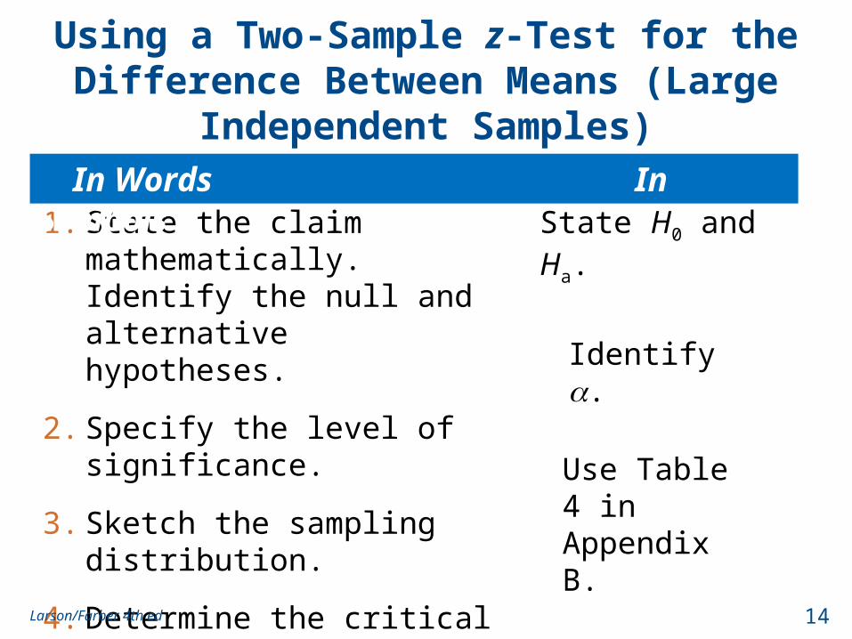
1. State the claim mathematically. Identify the null and alternative hypotheses.
2. Specify the level of significance.
3. Sketch the sampling distribution.
4. Determine the critical value(s).
5. Determine the rejection region(s).
State H0 and Ha.
Identify .
Use Table 4 in Appendix B.
In Words In Symbols
14Larson/Farber 4th ed
Using a Two-Sample z-Test for the Difference Between Means (Large
Independent Samples)
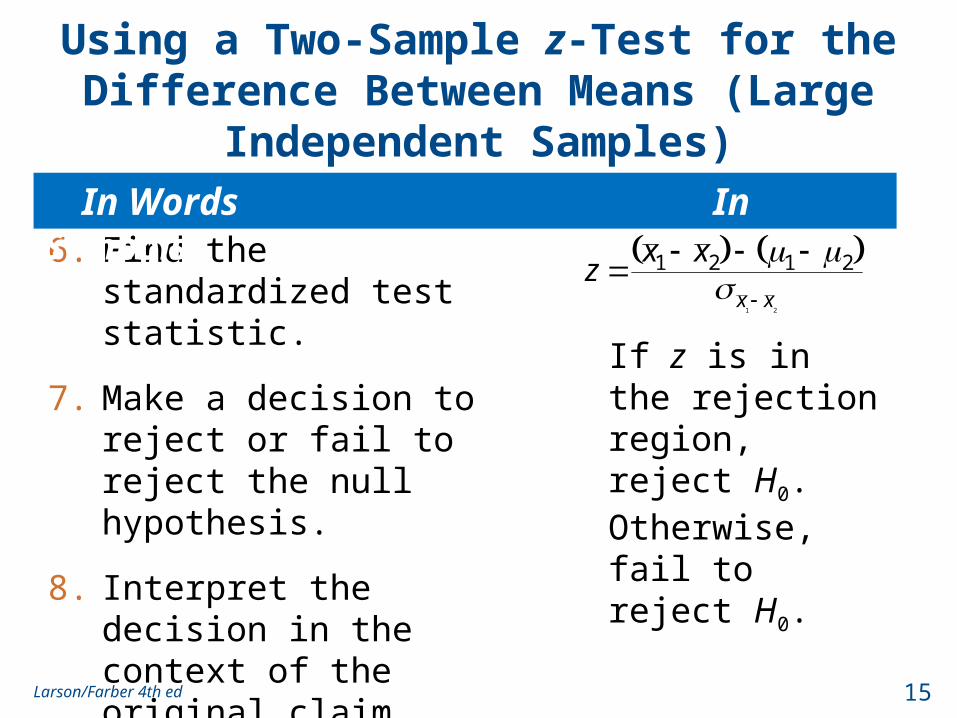
6. Find the standardized test statistic.
7. Make a decision to reject or fail to reject the null hypothesis.
8. Interpret the decision in the context of the original claim.
1 2
1 2 1 2
x x
x xz
If z is in the rejection region, reject H0.
Otherwise, fail to reject H0.
In Words In Symbols
15Larson/Farber 4th ed
Example: Two-Sample z-Test for the Difference Between Means
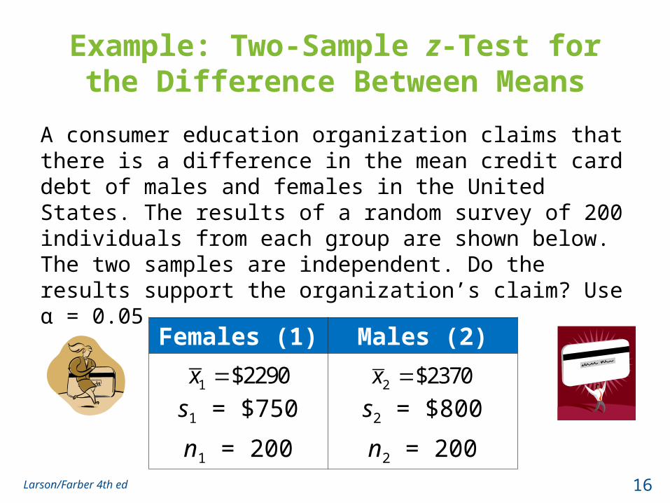
A consumer education organization claims that there is a difference in the mean credit card debt of males and females in the United States. The results of a random survey of 200 individuals from each group are shown below. The two samples are independent. Do the results support the organization’s claim? Use α = 0.05.
Females (1) Males (2)
s1 = $750 s2 = $800
n1 = 200 n2 = 200
1 $2290x 2 $2370x
16Larson/Farber 4th ed
Z0-1.96
0.025
1.96
0.025
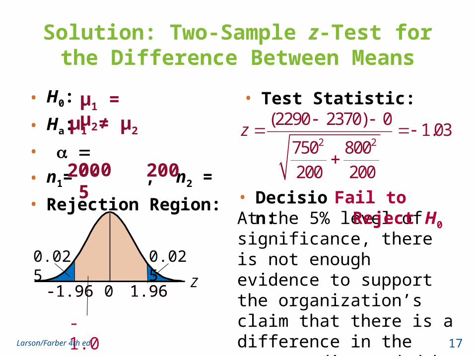
Solution: Two-Sample z-Test for the Difference Between Means
• H0:
• Ha:
•
• n1= , n2 =
• Rejection Region:
• Test Statistic:
0.05200 200
2 2
(2290 2370) 01.03
750 800
200 200
z
μ1 = μ2 μ1 ≠ μ2
-1.96 1.96
-1.03
• Decision:At the 5% level of significance, there is not enough evidence to support the organization’s claim that there is a difference in the mean credit card debt of males and females.
Fail to Reject H0
17Larson/Farber 4th ed
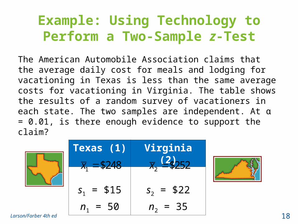
Example: Using Technology to Perform a Two-Sample z-Test
The American Automobile Association claims that the average daily cost for meals and lodging for vacationing in Texas is less than the same average costs for vacationing in Virginia. The table shows the results of a random survey of vacationers in each state. The two samples are independent. At α = 0.01, is there enough evidence to support the claim?
Texas (1) Virginia (2)
s1 = $15 s2 = $22
n1 = 50 n2 = 35
1 $248x 2 $252x
18Larson/Farber 4th ed
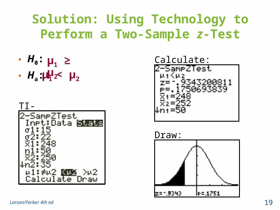
Solution: Using Technology to Perform a Two-Sample z-Test
• H0:
• Ha:
μ1 ≥ μ2 μ1 < μ2
TI-83/84set up:
Calculate:
Draw:
19Larson/Farber 4th ed
z0
0.01
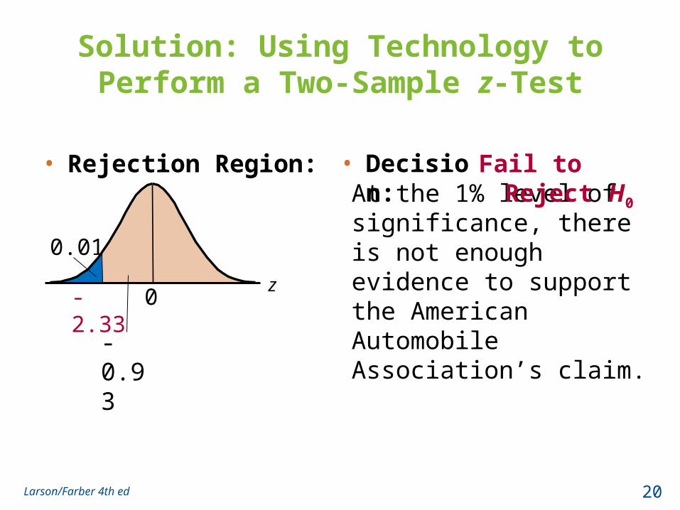
Solution: Using Technology to Perform a Two-Sample z-Test
• Decision:At the 1% level of significance, there is not enough evidence to support the American Automobile Association’s claim.
Fail to Reject H0• Rejection Region:
-0.93
-2.33
20Larson/Farber 4th ed
Section 8.1 Summary
• Determined whether two samples are independent or dependent
• Performed a two-sample z-test for the difference between two means μ1 and μ2 using large independent samples
21Larson/Farber 4th ed
Section 8.2
Testing the Difference Between Means (Small Independent Samples)
22Larson/Farber 4th ed
Section 8.2 Objectives
• Perform a t-test for the difference between two means μ1 and μ2 using small independent samples
23Larson/Farber 4th ed
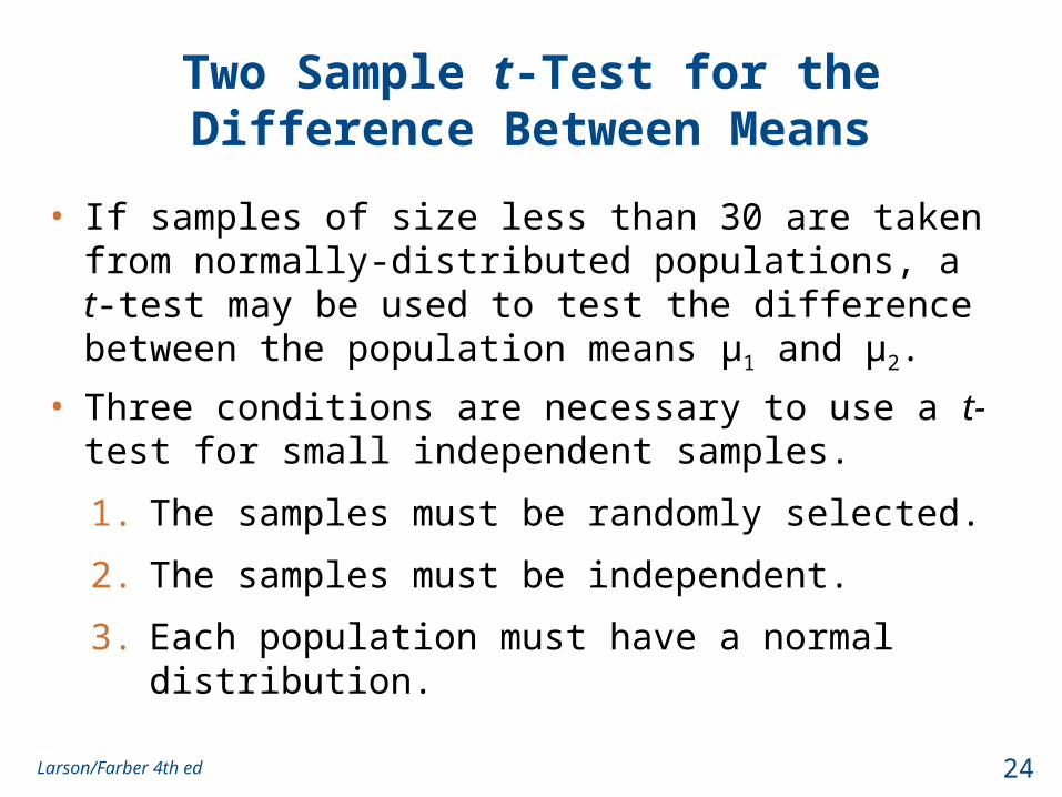
Two Sample t-Test for the Difference Between Means
• If samples of size less than 30 are taken from normally-distributed populations, a t-test may be used to test the difference between the population means μ1 and μ2.
• Three conditions are necessary to use a t-test for small independent samples.
1. The samples must be randomly selected.
2. The samples must be independent.
3. Each population must have a normal distribution.
24Larson/Farber 4th ed
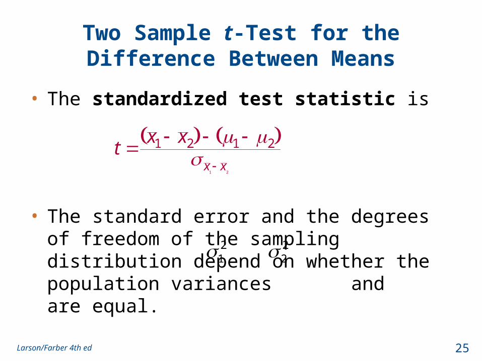
Two Sample t-Test for the Difference Between Means
• The standardized test statistic is
• The standard error and the degrees of freedom of the sampling distribution depend on whether the population variances and are equal.
1 2
1 2 1 2
x x
x xt
21 2
2
25Larson/Farber 4th ed
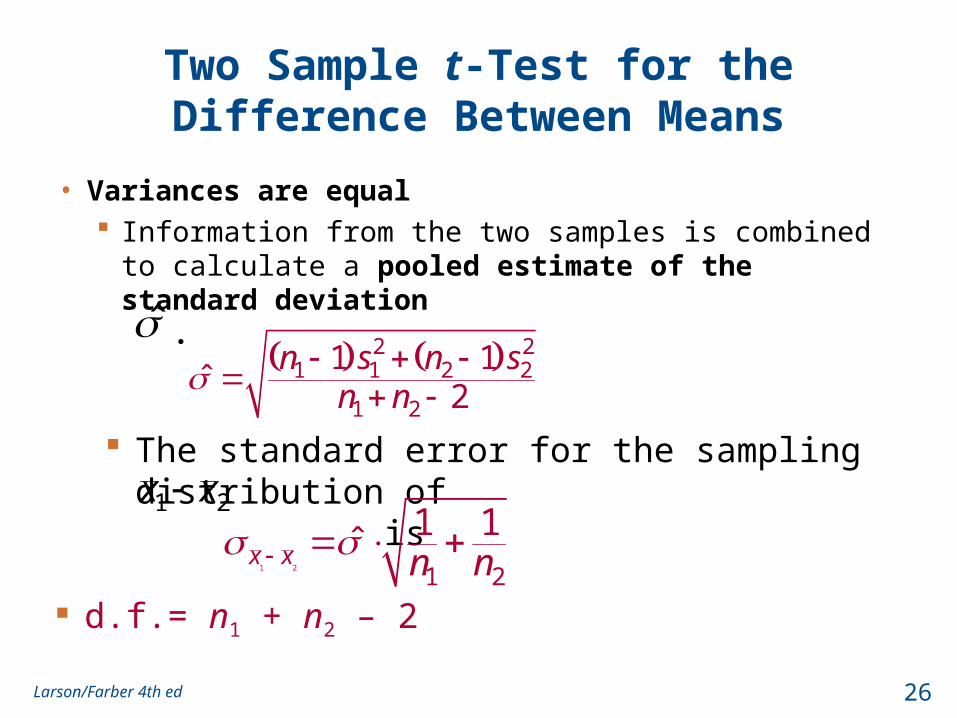
The standard error for the sampling distribution of is
Two Sample t-Test for the Difference Between Means
• Variances are equal Information from the two samples is combined to
calculate a pooled estimate of the standard deviation .
2 21 1 2 2
1 2
1 1ˆ 2
n s n sn n
1 2x x
1 2
1 2
1 1ˆx x n n
d.f.= n1 + n2 – 2
26Larson/Farber 4th ed
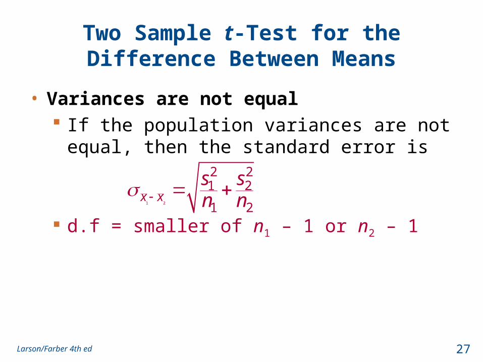
• Variances are not equal If the population variances are not equal, then the
standard error is
d.f = smaller of n1 – 1 or n2 – 1
Two Sample t-Test for the Difference Between Means
1 2
2 21 2
1 2x x
s sn n
27Larson/Farber 4th ed
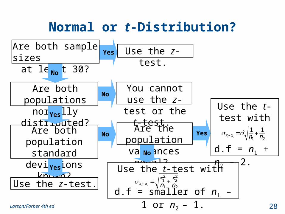
Normal or t-Distribution?
Are both sample sizes at least 30?
Are both populations normally distributed?
You cannot use the z-test or the t-test.
No
Yes
Are both population standard deviations
known?
Use the z-test.Yes
No
Are the population
variances equal?
Use the z-test.
Use the t-test with
d.f = smaller of n1 – 1 or n2 – 1.1 2
2 21 2
1 2 x x
s sn n
Use the t-test with
1 2
1 2
1 1 ˆx x n n
Yes
No
No
Yes
d.f = n1 + n2 – 2.
28Larson/Farber 4th ed
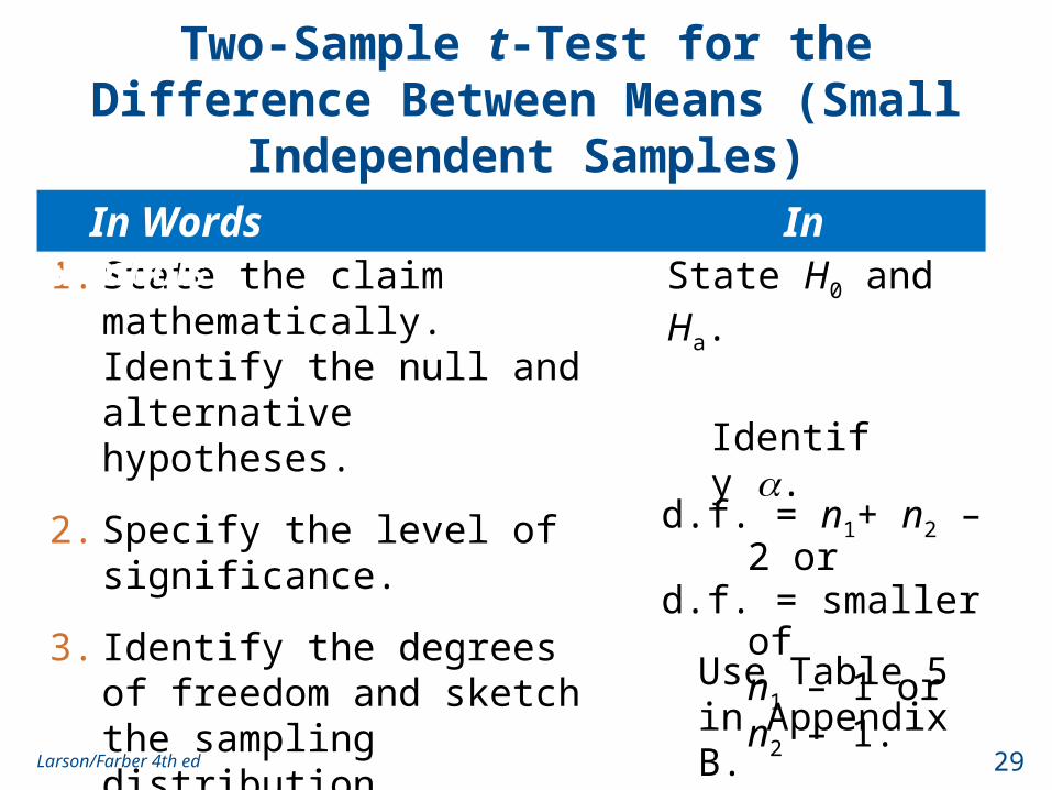
Two-Sample t-Test for the Difference Between Means (Small Independent
Samples)
1. State the claim mathematically. Identify the null and alternative hypotheses.
2. Specify the level of significance.
3. Identify the degrees of freedom and sketch the sampling distribution.
4. Determine the critical value(s).
State H0 and Ha.
Identify .
Use Table 5 in Appendix B.
d.f. = n1+ n2 – 2 ord.f. = smaller of
n1 – 1 or n2 – 1.
In Words In Symbols
29Larson/Farber 4th ed
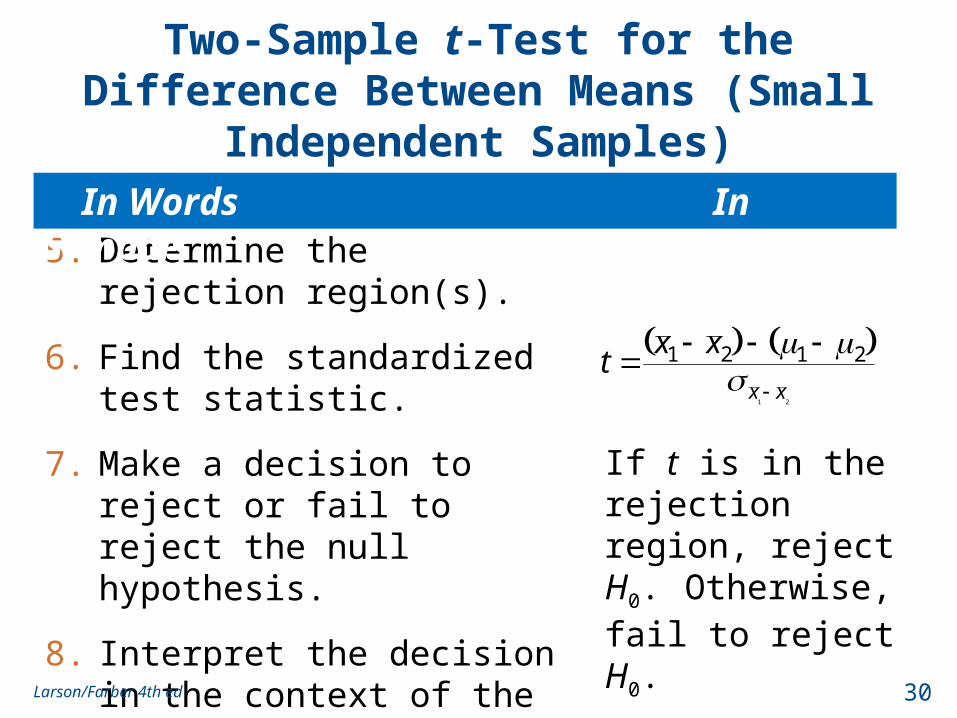
Two-Sample t-Test for the Difference Between Means (Small Independent
Samples)
5. Determine the rejection region(s).
6. Find the standardized test statistic.
7. Make a decision to reject or fail to reject the null hypothesis.
8. Interpret the decision in the context of the original claim.
1 2
1 2 1 2
x x
x xt
If t is in the rejection region, reject H0.
Otherwise, fail to reject H0.
In Words In Symbols
30Larson/Farber 4th ed
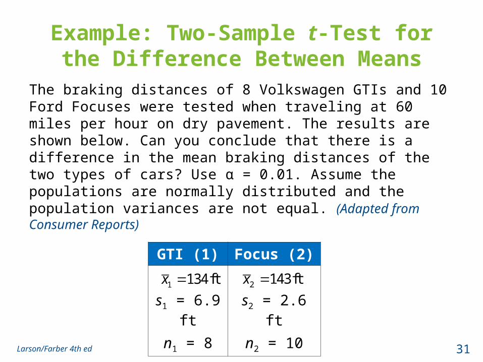
Example: Two-Sample t-Test for the Difference Between Means
The braking distances of 8 Volkswagen GTIs and 10 Ford Focuses were tested when traveling at 60 miles per hour on dry pavement. The results are shown below. Can you conclude that there is a difference in the mean braking distances of the two types of cars? Use α = 0.01. Assume the populations are normally distributed and the population variances are not equal. (Adapted from Consumer Reports)
GTI (1) Focus (2)
s1 = 6.9 ft s2 = 2.6 ft
n1 = 8 n2 = 10
1 134ftx 2 143ftx
31Larson/Farber 4th ed
t0-3.499
0.005
3.499
0.005
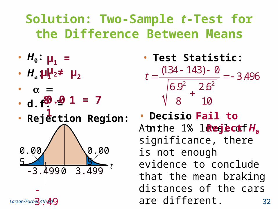
Solution: Two-Sample t-Test for the Difference Between Means
• H0:
• Ha:
•
• d.f. =
• Rejection Region:
• Test Statistic:
0.018 – 1 = 7
2 2
(134 143) 03.496
6.9 2.6
8 10
t
μ1 = μ2 μ1 ≠ μ2
-3.499 3.499
-3.496
• Decision:At the 1% level of significance, there is not enough evidence to conclude that the mean braking distances of the cars are different.
Fail to Reject H0
32Larson/Farber 4th ed
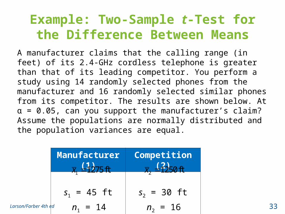
Example: Two-Sample t-Test for the Difference Between Means
A manufacturer claims that the calling range (in feet) of its 2.4-GHz cordless telephone is greater than that of its leading competitor. You perform a study using 14 randomly selected phones from the manufacturer and 16 randomly selected similar phones from its competitor. The results are shown below. At α = 0.05, can you support the manufacturer’s claim? Assume the populations are normally distributed and the population variances are equal.
Manufacturer (1) Competition (2)
s1 = 45 ft s2 = 30 ft
n1 = 14 n2 = 16
1 1275ftx 2 1250ftx
33Larson/Farber 4th ed
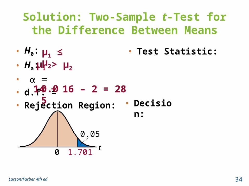
Solution: Two-Sample t-Test for the Difference Between Means
• H0:
• Ha:
•
• d.f. =
• Rejection Region:
• Test Statistic:
0.0514 + 16 – 2 = 28
μ1 ≤ μ2 μ1 > μ2
• Decision:
t0 1.701
0.05
34Larson/Farber 4th ed
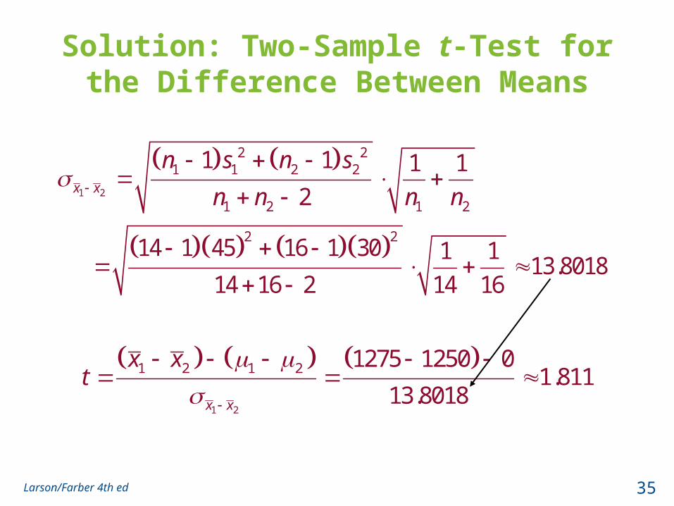
Solution: Two-Sample t-Test for the Difference Between Means
1 2
2 21 1 2 2
1 2 1 2
2 2
1 1 1 1
2
14 1 45 16 1 30 1 113.8018
14 16 2 14 16
x x
n s n s
n n n n
1 2
1 2 1 2 1275 1250 01.811
13.8018x x
x xt
35Larson/Farber 4th ed
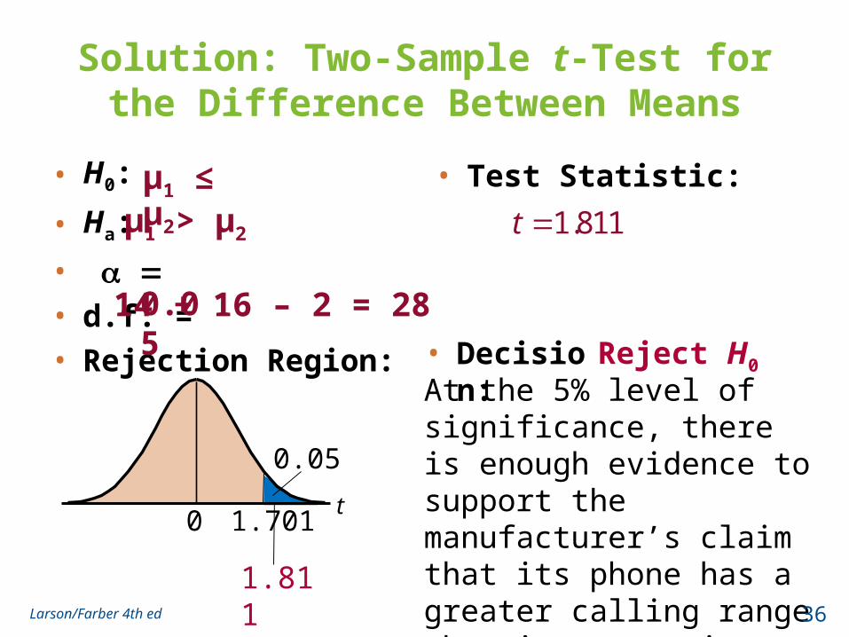
Solution: Two-Sample t-Test for the Difference Between Means
• H0:
• Ha:
•
• d.f. =
• Rejection Region:
• Test Statistic:
0.0514 + 16 – 2 = 28
1.811t μ1 ≤ μ2 μ1 > μ2
1.811
• Decision:At the 5% level of significance, there is enough evidence to support the manufacturer’s claim that its phone has a greater calling range than its competitors.
Reject H0
t0 1.701
0.05
36Larson/Farber 4th ed
Section 8.2 Summary
• Performed a t-test for the difference between two means μ1 and μ2 using small independent samples
37Larson/Farber 4th ed
Section 8.3
Testing the Difference Between Means (Dependent Samples)
38Larson/Farber 4th ed
Section 8.3 Objectives
• Perform a t-test to test the mean of the difference for a population of paired data
39Larson/Farber 4th ed
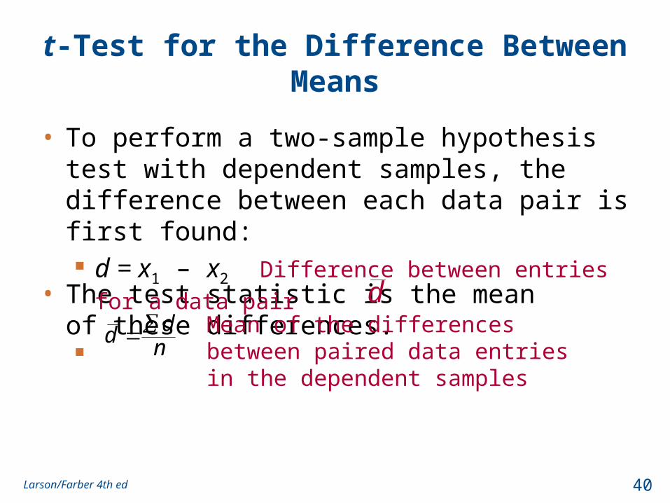
• The test statistic is the mean of these differences.
t-Test for the Difference Between Means
• To perform a two-sample hypothesis test with dependent samples, the difference between each data pair is first found: d = x1 – x2 Difference between entries for a data pair
ddd
n Mean of the differences between paired
data entries in the dependent samples
40Larson/Farber 4th ed
t-Test for the Difference Between Means
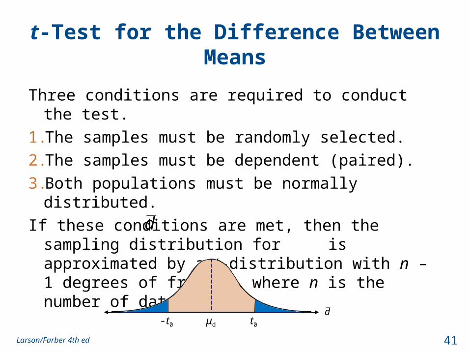
Three conditions are required to conduct the test.
1. The samples must be randomly selected.
2. The samples must be dependent (paired).
3. Both populations must be normally distributed.
If these conditions are met, then the sampling distribution for is approximated by a t-distribution with n – 1 degrees of freedom, where n is the number of data pairs.
d
d-t0 t0μd
41Larson/Farber 4th ed
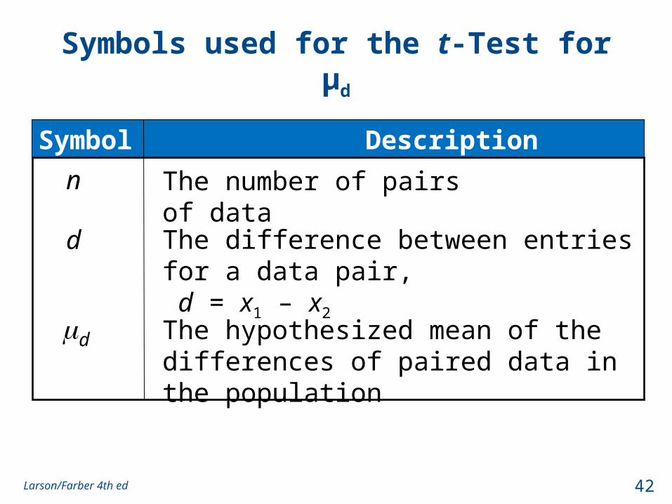
Symbols used for the t-Test for μd
The number of pairs of data
The difference between entries for a data pair, d = x1 – x2
d The hypothesized mean of the differences of paired data in the population
n
d
Symbol Description
42Larson/Farber 4th ed
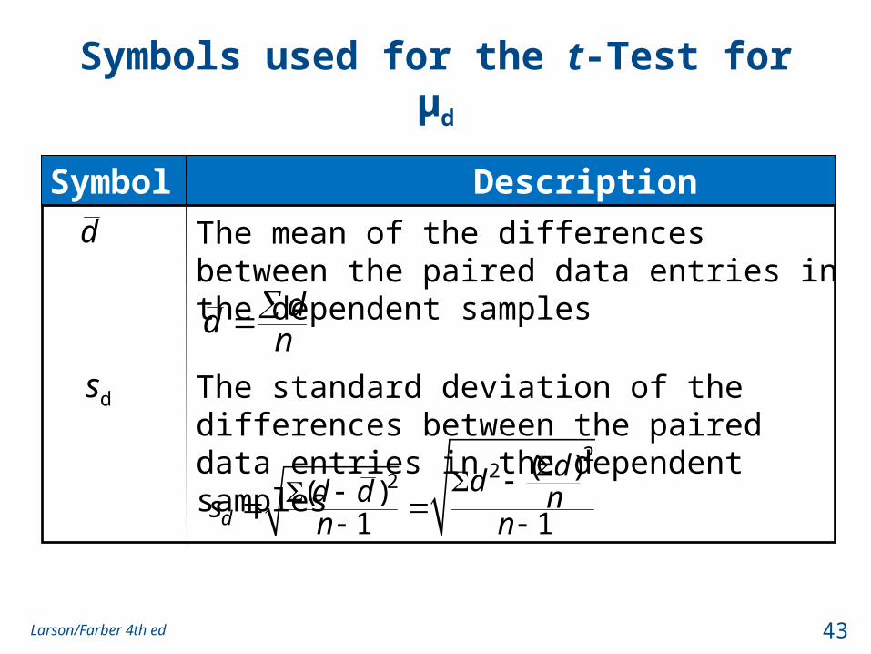
Symbols used for the t-Test for μd
Symbol Description
d The mean of the differences between the paired data entries in the dependent samples
The standard deviation of the differences between the paired data entries in the dependent samples
ddn
222
( )( )
1 1d
ddd d nsn n
sd
43Larson/Farber 4th ed
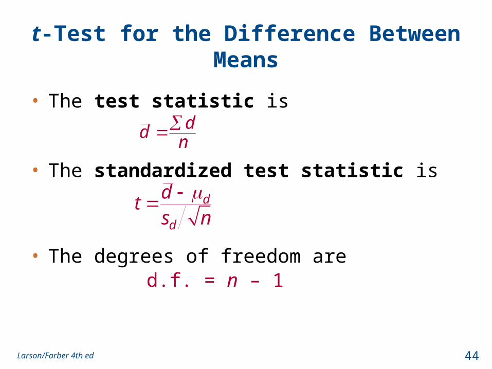
t-Test for the Difference Between Means
• The test statistic is
• The standardized test statistic is
• The degrees of freedom are d.f. = n – 1
d
d
dt
s n
ddn
44Larson/Farber 4th ed
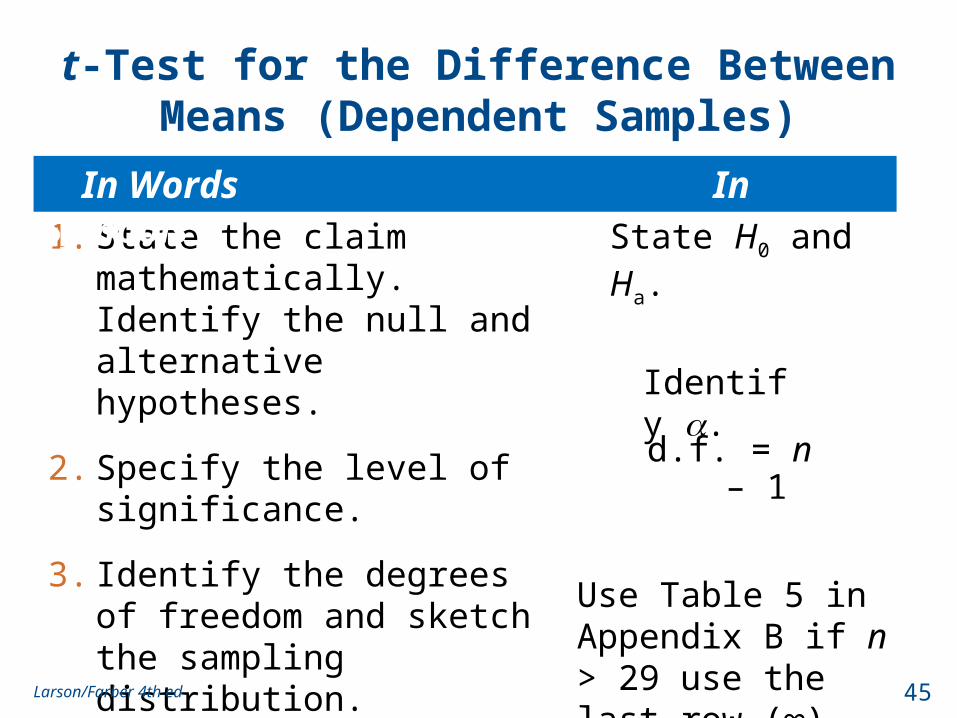
t-Test for the Difference Between Means (Dependent Samples)
1. State the claim mathematically. Identify the null and alternative hypotheses.
2. Specify the level of significance.
3. Identify the degrees of freedom and sketch the sampling distribution.
4. Determine the critical value(s).
State H0 and Ha.
Identify .
Use Table 5 in Appendix B if n > 29 use the last row (∞) .
d.f. = n – 1
In Words In Symbols
45Larson/Farber 4th ed
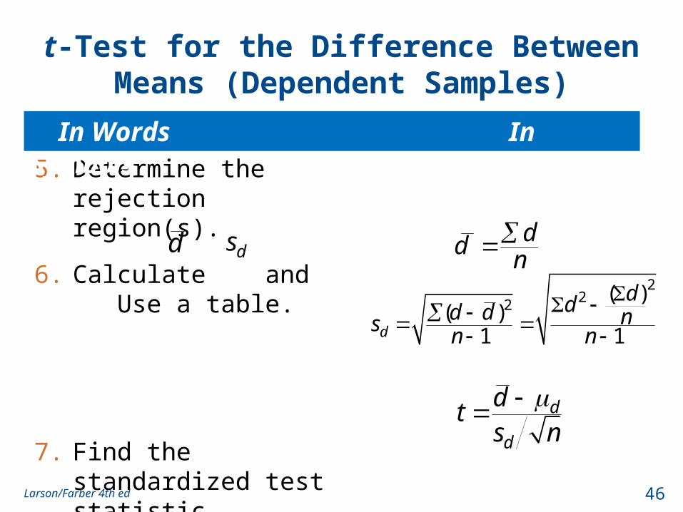
t-Test for the Difference Between Means (Dependent Samples)
5. Determine the rejection region(s).
6. Calculate and Use a table.
7. Find the standardized test statistic.
d .ds dn
d2
22( )
( )1 1d
ddd d nsn n
d
d
dt
s n
In Words In Symbols
46Larson/Farber 4th ed
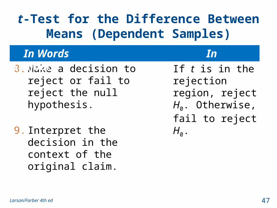
t-Test for the Difference Between Means (Dependent Samples)
8. Make a decision to reject or fail to reject the null hypothesis.
9. Interpret the decision in the context of the original claim.
If t is in the rejection region, reject H0.
Otherwise, fail to reject H0.
In Words In Symbols
47Larson/Farber 4th ed
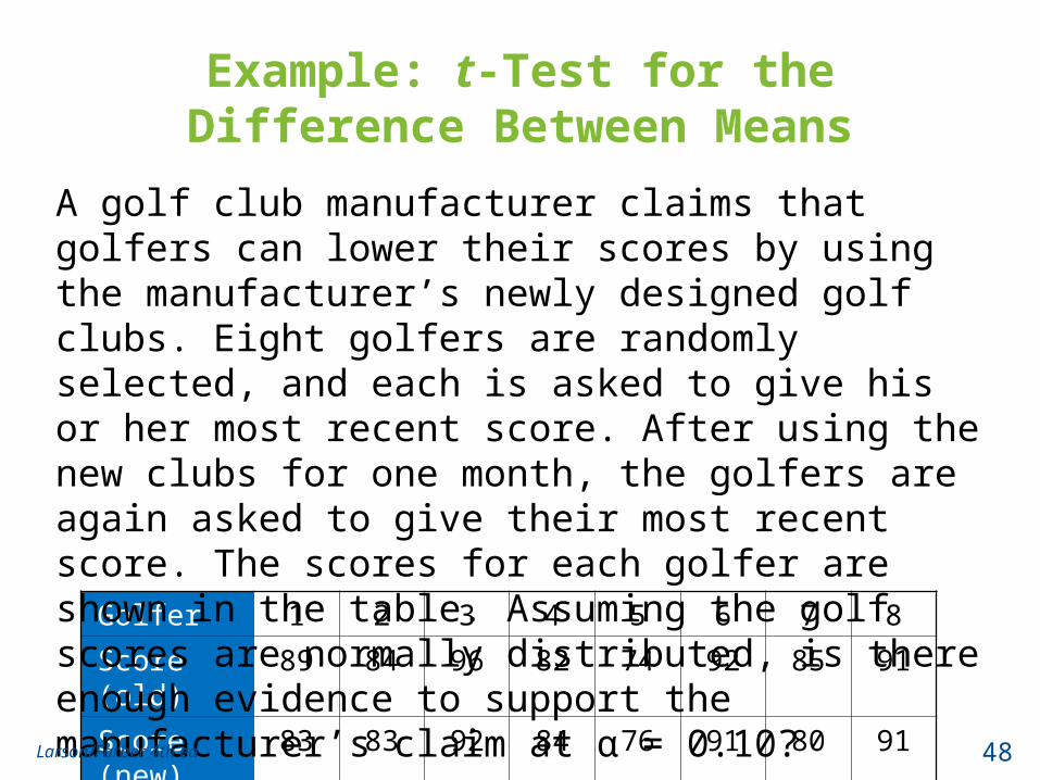
Example: t-Test for the Difference Between Means
Golfer 1 2 3 4 5 6 7 8
Score (old) 89 84 96 82 74 92 85 91
Score (new)
83 83 92 84 76 91 80 91
A golf club manufacturer claims that golfers can lower their scores by using the manufacturer’s newly designed golf clubs. Eight golfers are randomly selected, and each is asked to give his or her most recent score. After using the new clubs for one month, the golfers are again asked to give their most recent score. The scores for each golfer are shown in the table. Assuming the golf scores are normally distributed, is there enough evidence to support the manufacturer’s claim at α = 0.10?
48Larson/Farber 4th ed
t0 1.415
0.10
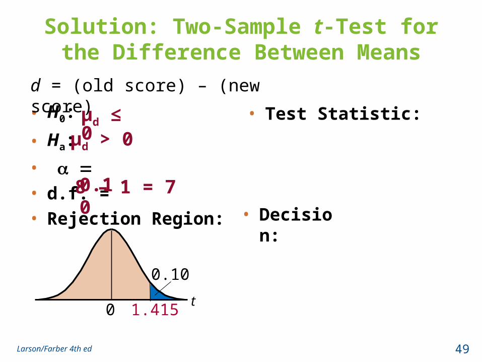
Solution: Two-Sample t-Test for the Difference Between Means
• H0:
• Ha:
•
• d.f. =
• Rejection Region:
• Test Statistic:
0.108 – 1 = 7
μd ≤ 0 μd > 0
• Decision:
d = (old score) – (new score)
49Larson/Farber 4th ed
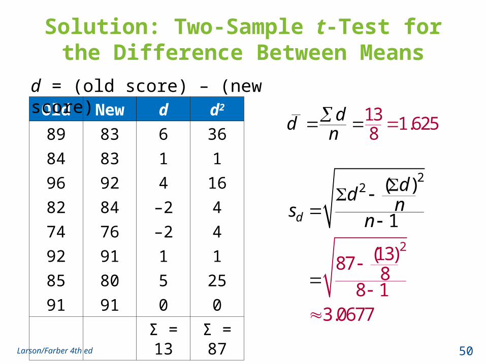
Solution: Two-Sample t-Test for the Difference Between Means
Old New d d2
89 83 6 36
84 83 1 1
96 92 4 16
82 84 –2 4
74 76 –2 4
92 91 1 1
85 80 5 25
91 91 0 0
Σ = 13 Σ = 87
13 1.6258
dn
d
2
2
2
(13)87
( )
1
88 1
3.0677
d
ddns
n
d = (old score) – (new score)
50Larson/Farber 4th ed
t0 1.415
0.10
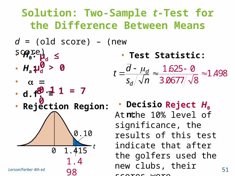
Solution: Two-Sample t-Test for the Difference Between Means
• H0:
• Ha:
•
• d.f. =
• Rejection Region:
• Test Statistic:
0.108 – 1 = 7
μd ≤ 0 μd > 0
1.415
• Decision:
d = (old score) – (new score)
1.625 0 1.4983.0677 8
d
d
dt
s n
1.498
At the 10% level of significance, the results of this test indicate that after the golfers used the new clubs, their scores were significantly lower.
Reject H0
51Larson/Farber 4th ed
Section 8.3 Summary
• Performed a t-test to test the mean of the difference for a population of paired data
52Larson/Farber 4th ed
Section 8.4
Testing the Difference Between Proportions
53Larson/Farber 4th ed
Section 8.4 Objectives
• Perform a z-test for the difference between two population proportions p1 and p2
54Larson/Farber 4th ed
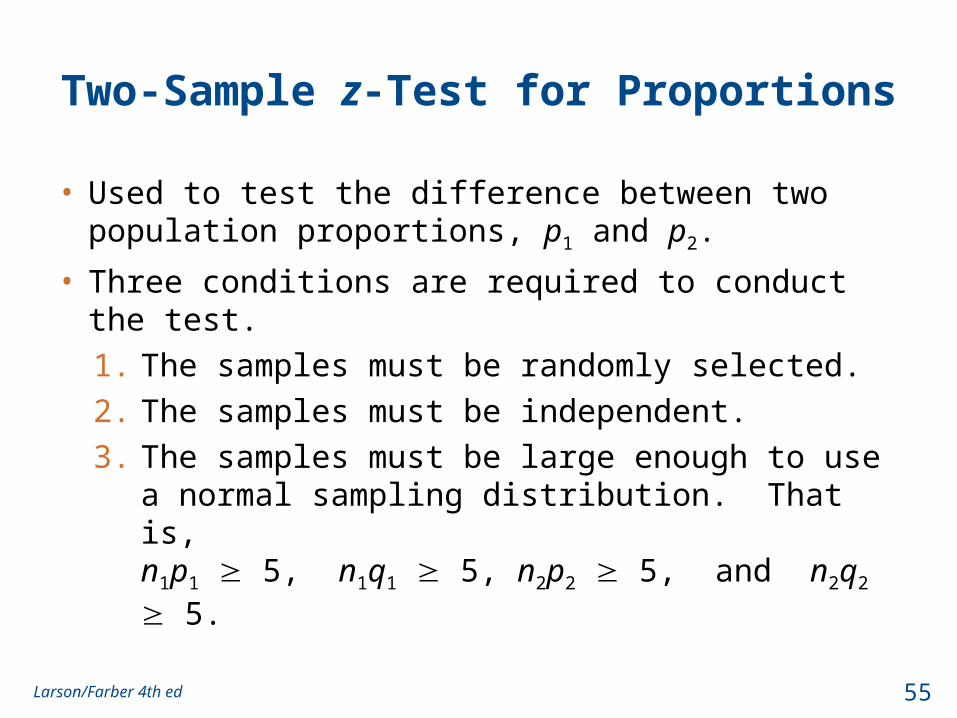
Two-Sample z-Test for Proportions
• Used to test the difference between two population proportions, p1 and p2.
• Three conditions are required to conduct the test.
1. The samples must be randomly selected.
2. The samples must be independent.
3. The samples must be large enough to use a normal sampling distribution. That is,n1p1 5, n1q1 5, n2p2 5, and n2q2 5.
55Larson/Farber 4th ed
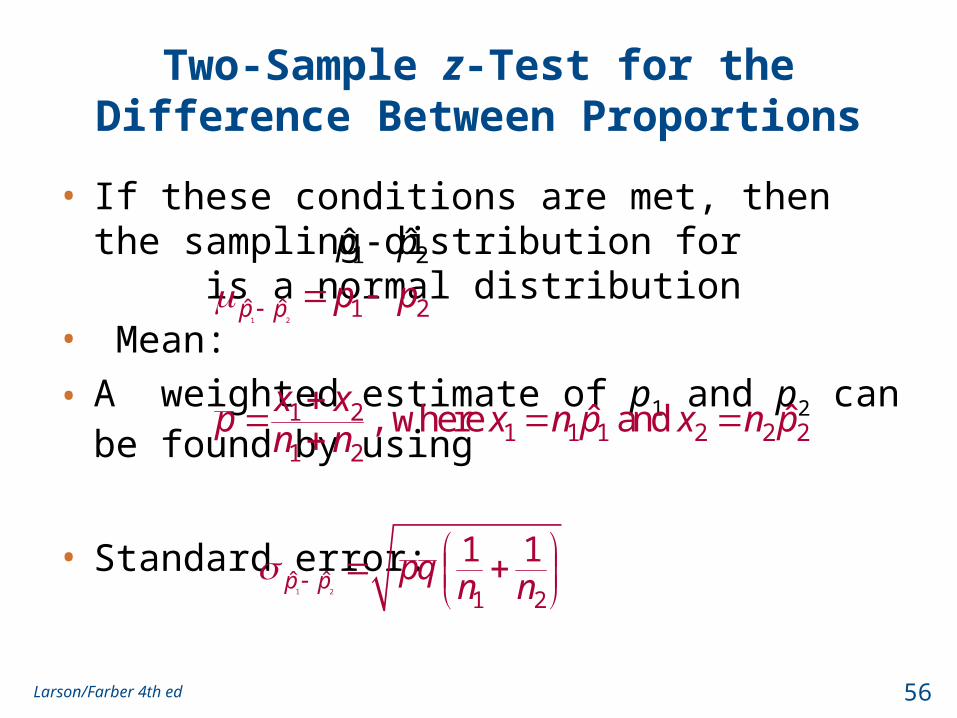
Two-Sample z-Test for the Difference Between Proportions
• If these conditions are met, then the sampling distribution for is a normal distribution
• Mean:
• A weighted estimate of p1 and p2 can be found by using
• Standard error:
1 2ˆ ˆp p
1 21 2ˆ ˆp p p p
1 2ˆ ˆ
1 2
1 1p p pq
n n
1 21 1 1 2 2 2
1 2, where and ˆ ˆ
x xp x n p x n p
n n
56Larson/Farber 4th ed
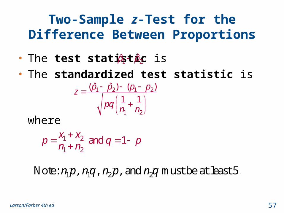
Two-Sample z-Test for the Difference Between Proportions
• The test statistic is
• The standardized test statistic is
where
1 2 1 2
1 2
( ) ( )ˆ ˆ
1 1
p p p pz
pqn n
1 2ˆ ˆp p
1 2
1 2 and 1
x xp q p
n n
1 1 2 2Note: , , , and must be at least 5.n p n q n p n q
57Larson/Farber 4th ed
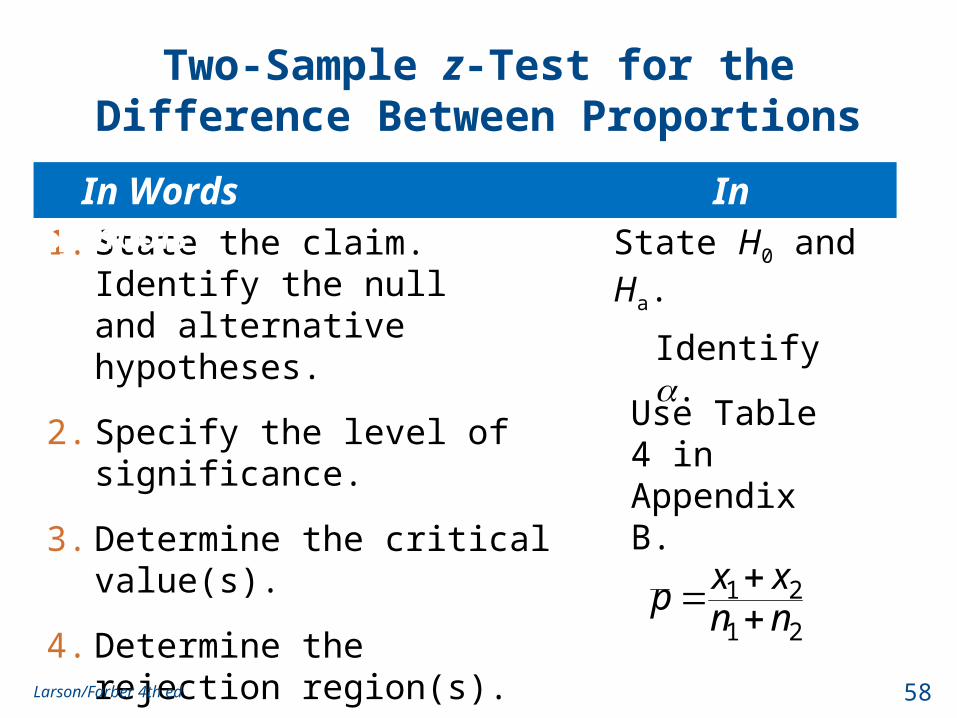
Two-Sample z-Test for the Difference Between Proportions
1. State the claim. Identify the null and alternative hypotheses.
2. Specify the level of significance.
3. Determine the critical value(s).
4. Determine the rejection region(s).
5. Find the weighted estimate of p1 and p2.
State H0 and Ha.
Identify .
Use Table 4 in Appendix B.
1 2
1 2
x xp
n n
In Words In Symbols
58Larson/Farber 4th ed
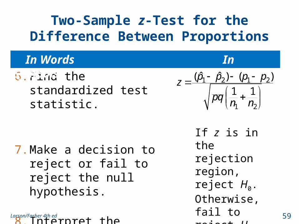
Two-Sample z-Test for the Difference Between Proportions
6. Find the standardized test statistic.
7. Make a decision to reject or fail to reject the null hypothesis.
8. Interpret the decision in the context of the original claim.
1 2 1 2
1 2
( ) ( )ˆ ˆ
1 1
p p p pz
pqn n
If z is in the rejection region, reject H0.
Otherwise, fail to reject H0.
In Words In Symbols
59Larson/Farber 4th ed
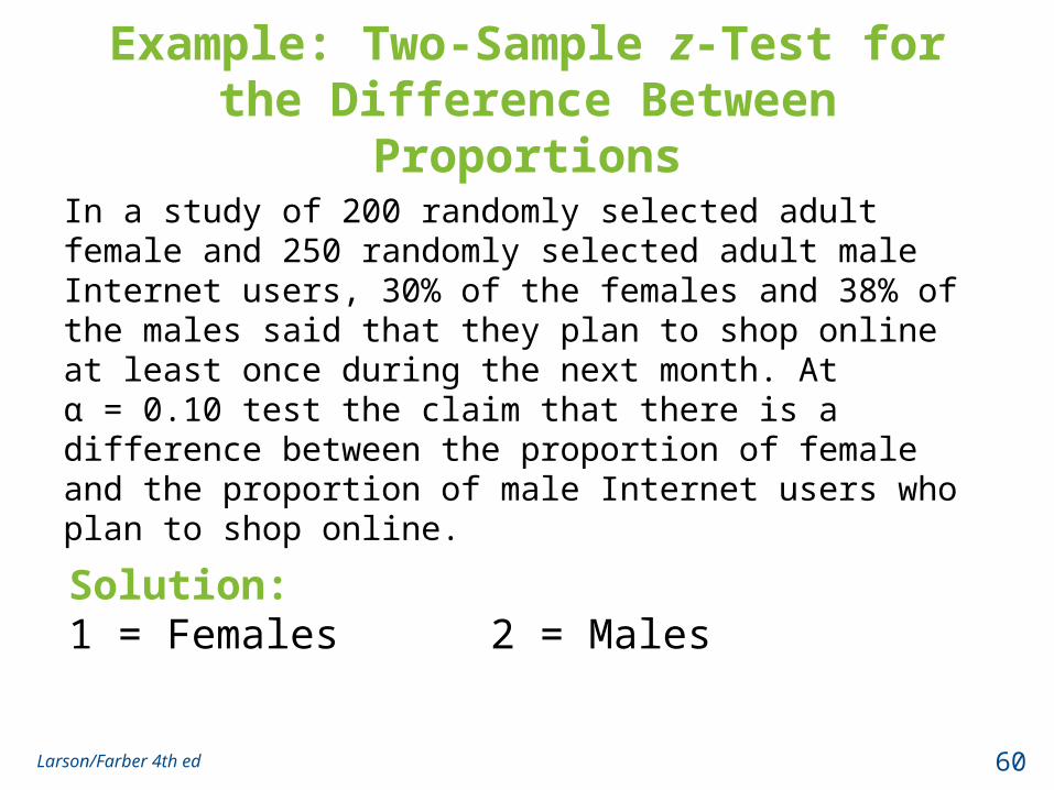
Example: Two-Sample z-Test for the Difference Between Proportions
In a study of 200 randomly selected adult female and 250 randomly selected adult male Internet users, 30% of the females and 38% of the males said that they plan to shop online at least once during the next month. At α = 0.10 test the claim that there is a difference between the proportion of female and the proportion of male Internet users who plan to shop online.
Solution: 1 = Females 2 = Males
60Larson/Farber 4th ed
Z0-1.645
0.05
1.645
0.05
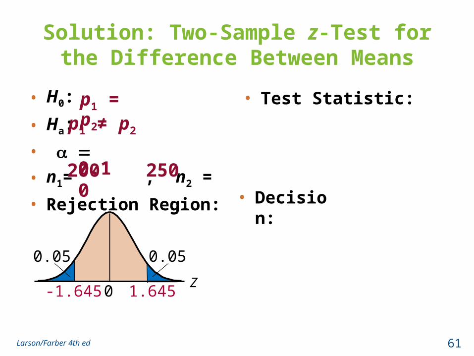
Solution: Two-Sample z-Test for the Difference Between Means
• H0:
• Ha:
•
• n1= , n2 =
• Rejection Region:
• Test Statistic:
0.10200 250
p1 = p2 p1 ≠ p2
• Decision:
61Larson/Farber 4th ed
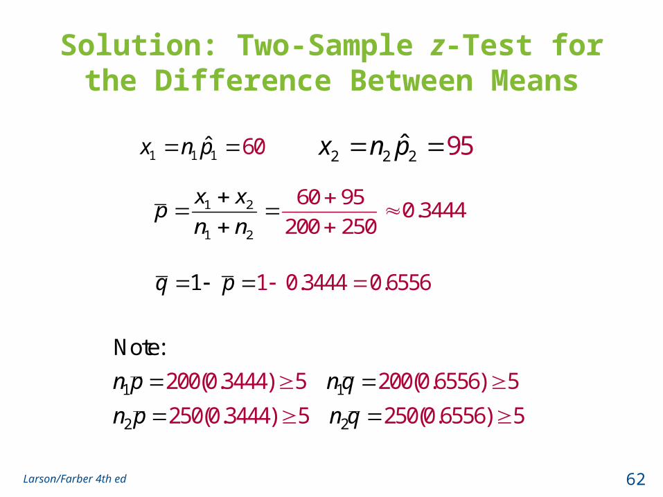
Solution: Two-Sample z-Test for the Difference Between Means
1 2
1 2
60 95 0.3444
200 250
x xp
n n
1 1 1ˆ 60x n p 2 2 2ˆ 95x n p
1 0.3444 01 .6556q p
1 1
2 2
200(0.3444) 5 200(0.6556) 5
250(0.3444) 5
N
250(
ote:
0.6556) 5
n p n q
n p n q
62Larson/Farber 4th ed

Solution: Two-Sample z-Test for the Difference Between Means
1 2 1 2
1 2
0.30 0.38 0
1 10.3444 0.6556
200
ˆ ˆ
1 1250
1.77
p p p pz
pqn n
63Larson/Farber 4th ed
z0-1.645
0.05
1.645
0.05
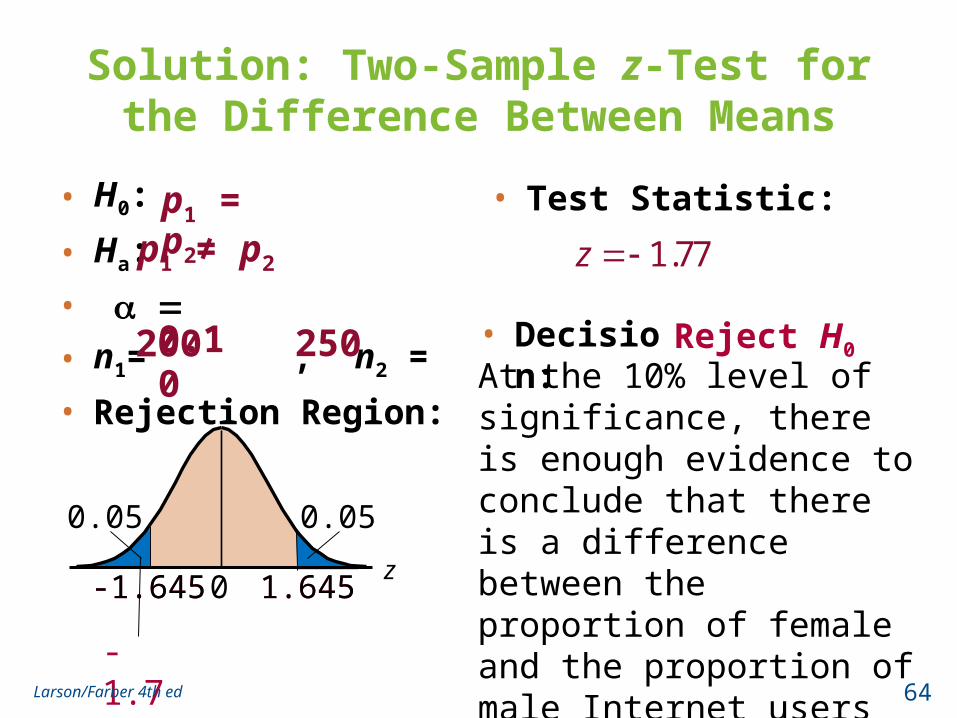
Solution: Two-Sample z-Test for the Difference Between Means
• H0:
• Ha:
•
• n1= , n2 =
• Rejection Region:
• Test Statistic:
0.10200 250
1.77z p1 = p2 p1 ≠ p2
-1.645 1.645
-1.77
• Decision:At the 10% level of significance, there is enough evidence to conclude that there is a difference between the proportion of female and the proportion of male Internet users who plan to shop online.
Reject H0
64Larson/Farber 4th ed
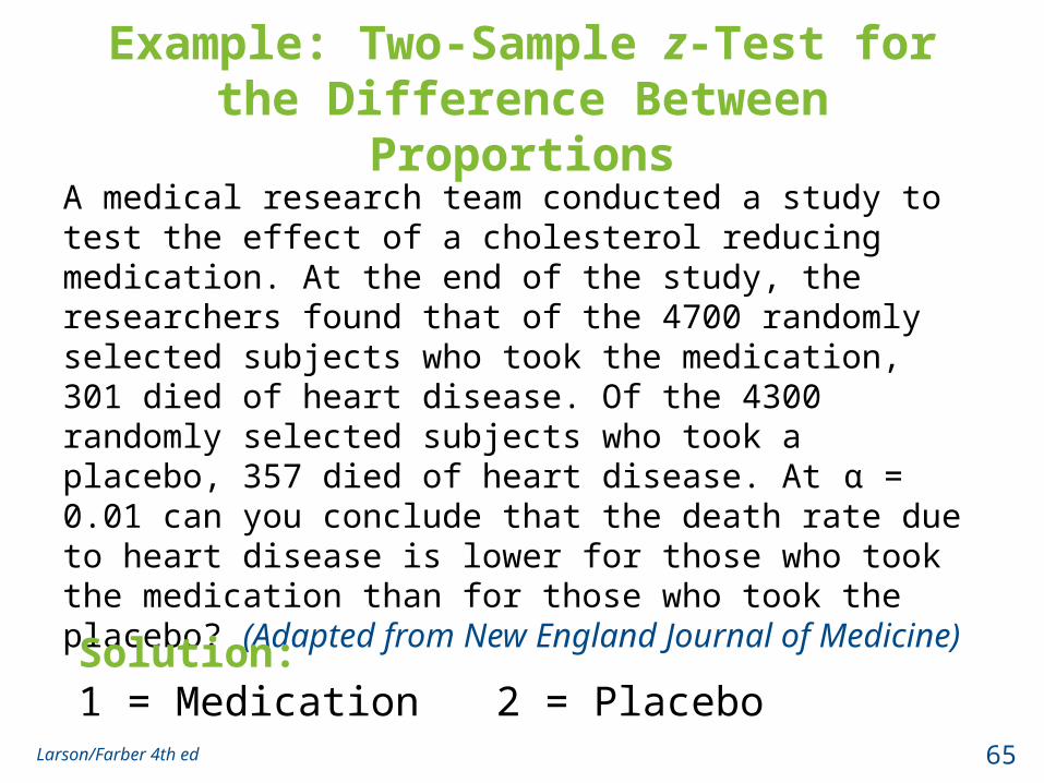
Example: Two-Sample z-Test for the Difference Between Proportions
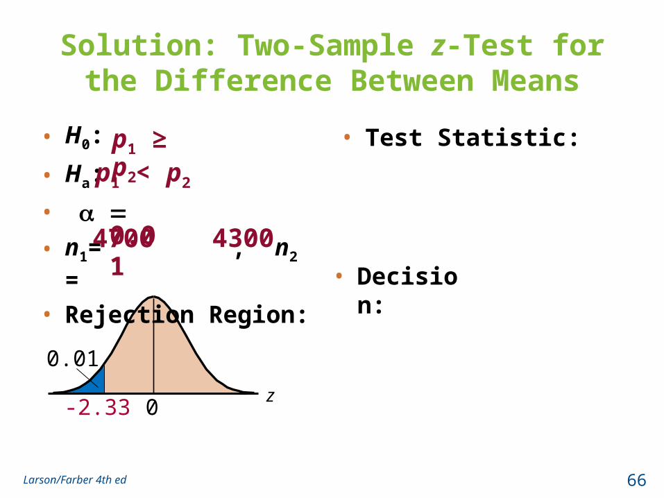
A medical research team conducted a study to test the effect of a cholesterol reducing medication. At the end of the study, the researchers found that of the 4700 randomly selected subjects who took the medication, 301 died of heart disease. Of the 4300 randomly selected subjects who took a placebo, 357 died of heart disease. At α = 0.01 can you conclude that the death rate due to heart disease is lower for those who took the medication than for those who took the placebo? (Adapted from New England Journal of Medicine)Solution: 1 = Medication 2 = Placebo
65Larson/Farber 4th ed
z0-2.33
0.01
Solution: Two-Sample z-Test for the Difference Between Means
• H0:
• Ha:
•
• n1= , n2 =
• Rejection Region:
• Test Statistic:
0.014700 4300
p1 ≥ p2 p1 < p2
• Decision:
66Larson/Farber 4th ed
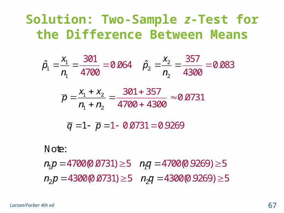
Solution: Two-Sample z-Test for the Difference Between Means
1 2
1 2
301 357 0.0731
4700 4300
x xp
n n
11
1
3010.064
470ˆ
0
xp
n
1 0.0731 01 .9269q p
22
2
3570.083
430ˆ
0
xp
n
1 1
2 2
4700(0.0731) 5 4700(0.9269) 5
4300(0.0731
Note:
) 5 4300(0.926
9) 5
n p n q
n p n q
67Larson/Farber 4th ed

Solution: Two-Sample z-Test for the Difference Between Means
1 2 1 2
1 2
0.064 0.083 0
1 10.0731 0.92
ˆ
694700 4300
3.
ˆ
1
6
1
4
p p p pz
pqn n
68Larson/Farber 4th ed
z0-2.33
0.01
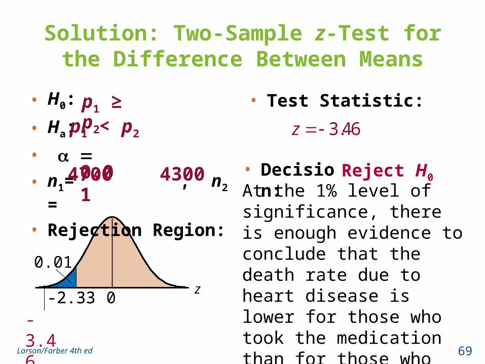
Solution: Two-Sample z-Test for the Difference Between Means
• H0:
• Ha:
•
• n1= , n2 =
• Rejection Region:
• Test Statistic:
0.014700 4300
3.46z p1 ≥ p2 p1 < p2
-2.33
-3.46
• Decision:At the 1% level of significance, there is enough evidence to conclude that the death rate due to heart disease is lower for those who took the medication than for those who took the placebo.
Reject H0
69Larson/Farber 4th ed
Section 8.4 Summary
• Performed a z-test for the difference between two population proportions p1 and p2
70Larson/Farber 4th ed