Embed Size (px)
Citation preview
8–1
8 Relaxation†
Relaxation is the process by which the spins in the sample come to equilibriumwith the surroundings. At a practical level, the rate of relaxation determineshow fast an experiment can be repeated, so it is important to understand howrelaxation rates can be measured and the factors that influence their values.The rate of relaxation is influenced by the physical properties of the moleculeand the sample, so a study of relaxation phenomena can lead to information onthese properties. Perhaps the most often used and important of thesephenomena in the nuclear Overhauser effect (NOE) which can be used to probeinternuclear distances in a molecule. Another example is the use of data onrelaxation rates to probe the internal motions of macromolecules.
In this chapter the language and concepts used to describe relaxation will beintroduced and illustrated. To begin with it will simply be taken for grantedthat there are processes which give rise to relaxation and we will not concernourselves with the source of relaxation. Having described the experimentswhich can be used to probe relaxation we will then go on to see what the sourceof relaxation is and how it depends on molecular parameters and molecularmotion.
8.1 What is relaxation?
Relaxation is the process by which the spins return to equilibrium. Equilibriumis the state in which (a) the populations of the energy levels are those predictedby the Boltzmann distribution and (b) there is no transverse magnetization and,more generally, no coherences present in the system.
In Chapter 3 we saw that when an NMR sample is placed in a staticmagnetic field and allowed to come to equilibrium it is found that a netmagnetization of the sample along the direction of the applied field(traditionally the z-axis) is developed. Magnetization parallel to the appliedfield is termed longitudinal.
This equilibrium magnetization arises from the unequal population of thetwo energy levels that correspond to the α and β spin states. In fact, the z-magnetization, Mz, is proportional to the population difference
M n nz ∝ −( )α β
where nα and nβ are the populations of the two corresponding energy levels.Ultimately, the constant of proportion just determines the absolute size of thesignal we will observe. As we are generally interested in the relative size ofmagnetizations and signals we may just as well write
M n nz = −( )α β [2]
† Chapter 8 "Relaxation" © James Keeler 1999 and 2002
α
β
x y
z
A population difference givesrise to net magnetization alongthe z-axis.
8–2
8.2 Rate equations and rate constants
The populations of energy levels are in many ways analogous to concentrationsin chemical kinetics, and many of the same techniques that are used to describethe rates of chemical reactions can also be used to describe the dynamics ofpopulations. This will lead to a description of the dynamics of the z-magnetization.
Suppose that the populations of the α and β states at time t are nα and nβ,respectively. If these are not the equilibrium values, then for the system toreach equilibrium the population of one level must increase and that of the othermust decrease. This implies that there must be transitions between the twolevels i.e. something must happen which causes a spin to move from the α stateto the β state or vice versa. It is this process which results in relaxation.
The simplest assumption that we can make about the rate of transitions fromα to β is that it is proportional to the population of state α, nα, and is a firstorder process with rate constant W. With these assumptions the rate of loss ofpopulation from state α is Wnα. In the same way, the rate of loss of populationof state β is Wnβ.
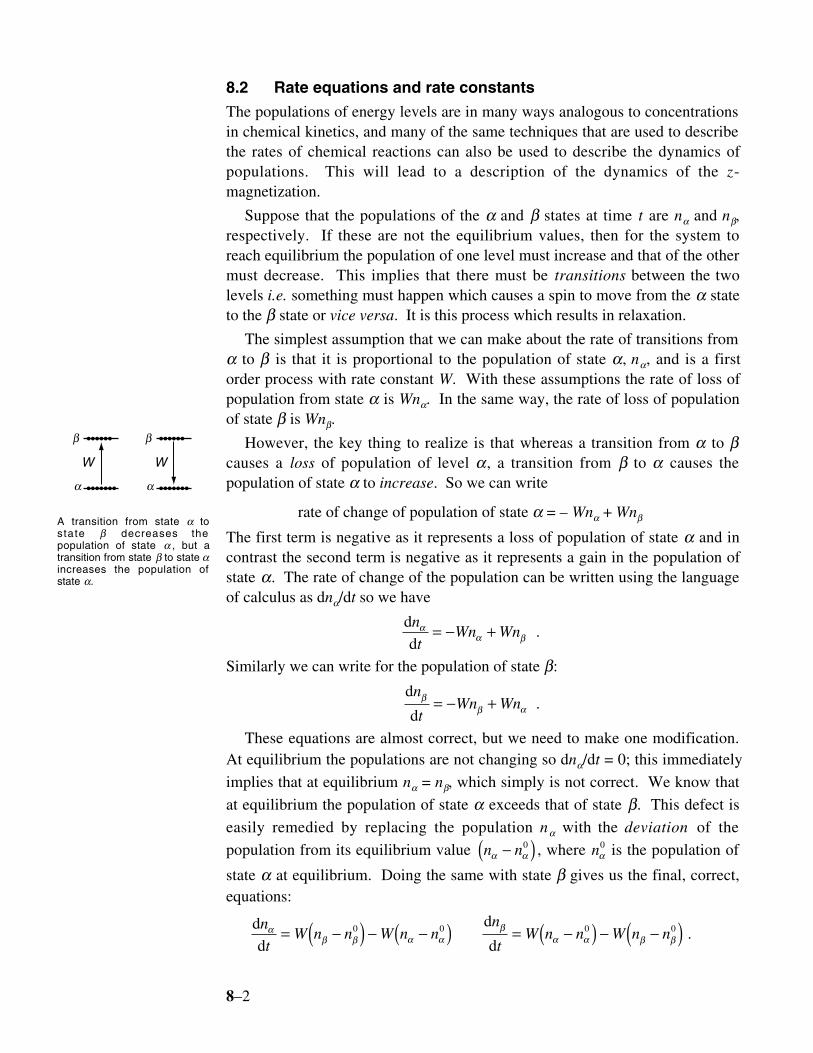
However, the key thing to realize is that whereas a transition from α to βcauses a loss of population of level α, a transition from β to α causes thepopulation of state α to increase. So we can write
rate of change of population of state α = – Wnα + Wnβ
The first term is negative as it represents a loss of population of state α and incontrast the second term is negative as it represents a gain in the population ofstate α. The rate of change of the population can be written using the languageof calculus as dnα/dt so we have
ddn
tWn Wnα
α β= − + .
Similarly we can write for the population of state β:
d
d
n
tWn Wnβ
β α= − + .
These equations are almost correct, but we need to make one modification.At equilibrium the populations are not changing so dnα/dt = 0; this immediately
implies that at equilibrium nα = nβ, which simply is not correct. We know that
at equilibrium the population of state α exceeds that of state β. This defect is
easily remedied by replacing the population nα with the deviation of the
population from its equilibrium value n nα α−( )0 , where nα0 is the population of
state α at equilibrium. Doing the same with state β gives us the final, correct,equations:
dd
d
dn
tW n n W n n
n
tW n n W n nα
β β α αβ
α α β β= −( ) − −( ) = −( ) − −( )0 0 0 0 .
α
β
W
α
β
W
A transition from state α tostate β decreases thepopulation of state α , but atransition from state β to state αincreases the population ofstate α.
8–3
You will recognise here that this kind of approach is exactly the same as thatused to analyse the kinetics of a reversible chemical reaction.
Using Eqn. [2], we can use these two equations to work out how the z-magnetization varies with time:
dd
d
d
dd
d
d
M
t
n n
t
n
t
n
t
W n n W n n W n n W n n
W n n W n n
W M M
z
z z
=−( )
= −
= −( ) − −( ) − −( ) + −( )= − −( ) + −( )= − −( )
α β
α β
β β α α α α β β
α β α β
0 0 0 0
0 0
0
2 2
2
where M n nz0 0 0= −( )α β , the equilibrium z-magnetization.
8.2.1 Consequences of the rate equation
The discussion in the previous section led to a (differential) equation describingthe motion of the z-magnetization
dd
M t
tR M t Mz
z z z
( ) = − ( ) −( )0 [7]
where the rate constant, Rz = 2W and Mz has been written as a function of time,Mz(t), to remind us that it may change.
What this equations says is that the rate of change of Mz is proportional tothe deviation of Mz from its equilibrium value, Mz
0 . If Mz = Mz0 , that is the
system is at equilibrium, the right-hand side of Eqn. [7] is zero and hence so isthe rate of change of Mz: nothing happens. On the other hand, if Mz deviatesfrom Mz
0 there will be a rate of change of Mz, and this rate will be proportionalto the deviation of Mz from Mz
0 . The change will also be such as to return Mz toits equilibrium value, Mz
0 . In summary, Eqn. [7] predicts that over time Mz willreturn to Mz
0 ; this is exactly what we expect. The rate at which this happenswill depend on Rz.
This equation can easily be integrated:
dd
const.
M t
M t MR t
M t M R t
z
z zz
z z z
( )( ) −( ) = −
( ) −( ) = − +
∫ ∫0
0ln
If, at time zero, the magnetization is Mz(0), the constant of integration can bedetermined as ln M Mz z0 0( ) −( ). Hence, with some rearrangement:
8–4
lnM t M
M MR tz z
z zz
( ) −( ) −
= −
0
00[7A]
or
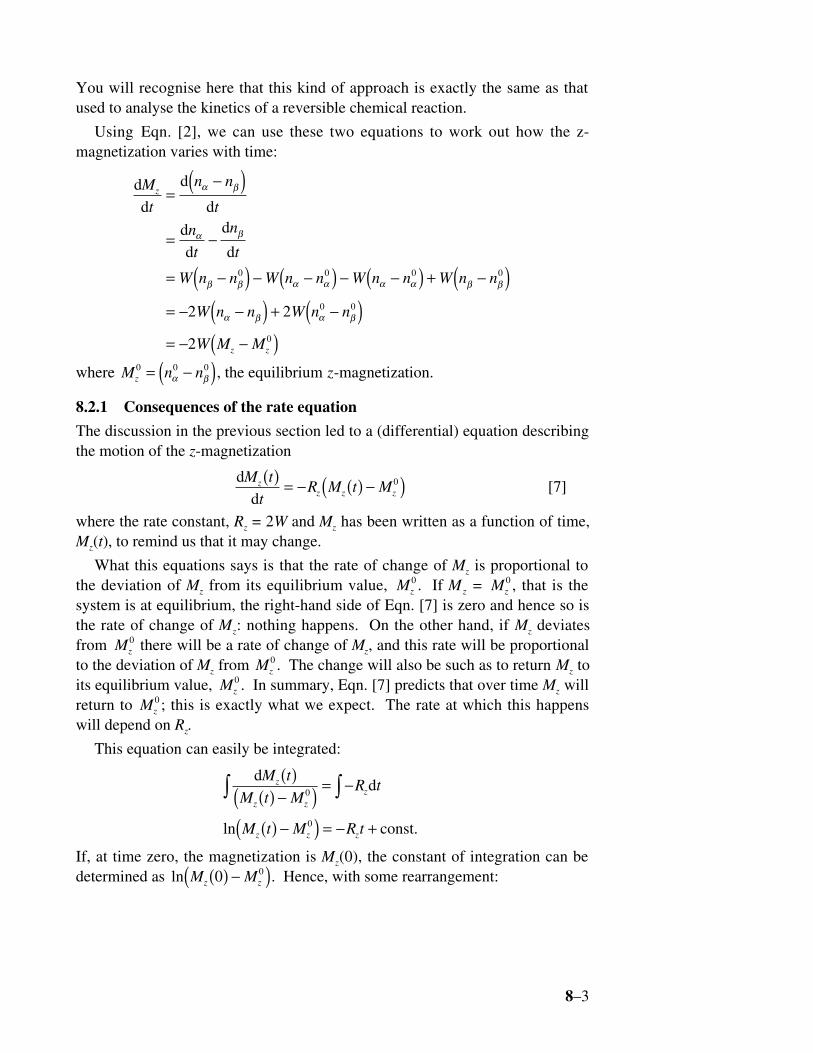
M t M M R t Mz z z z z( ) = ( ) −[ ] −( ) +0 0 0exp [7B]
In words, this says that the z-magnetization returns from Mz(0) to Mz0 following
an exponential law. The time constant of the exponential is 1/Rz, and this isoften called T1, the longitudinal or spin-lattice relaxation time.
8.2.2 The inversion recovery experiment
We described this experiment in section 3.10. First, a 180° pulse is applied,thereby inverting the magnetization. Then a delay t is left for the magnetizationto relax. Finally, a 90° pulse is applied so that the size of the z-magnetizationcan be measured.
We can now analyse this experiment fully. The starting condition for Mz isM Mz z0 0( ) = − , i.e. inversion. With this condition the predicted time evolutioncan be found from Eqn. [7A] to be:
lnM t M
MR tz z
zz
( ) −−
= −
0
02
Recall that the amplitude of the signal we record in this experiment isproportional to the z-magnetization. So, if this signal is S(t) it follows that
lnS t S
SR tz
( ) −−
= −0
02[7C]
where S0 is the signal intensity from equilibrium magnetization; we would findthis from a simple 90° – acquire experiment.
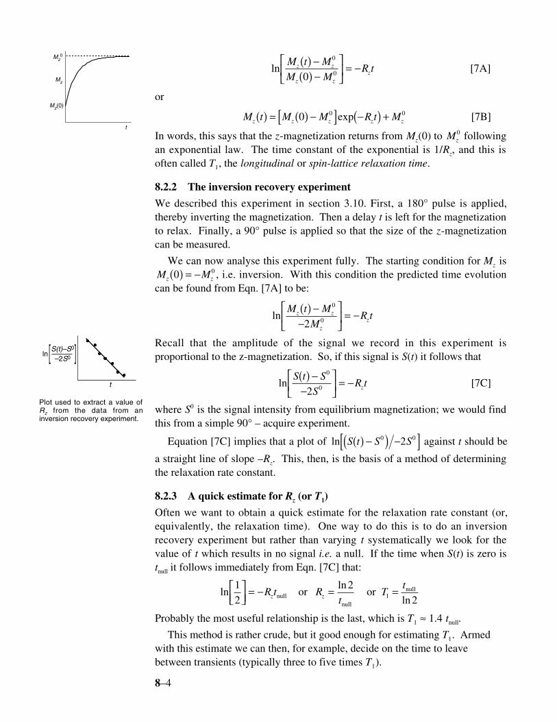
Equation [7C] implies that a plot of ln S t S S( ) −( ) −[ ]0 02 against t should be
a straight line of slope –Rz. This, then, is the basis of a method of determiningthe relaxation rate constant.
8.2.3 A quick estimate for Rz (or T1)
Often we want to obtain a quick estimate for the relaxation rate constant (or,equivalently, the relaxation time). One way to do this is to do an inversionrecovery experiment but rather than varying t systematically we look for thevalue of t which results in no signal i.e. a null. If the time when S(t) is zero istnull it follows immediately from Eqn. [7C] that:
lnln
ln12
221
= − = =R t Rt
Tt
z znullnull
null or or
Probably the most useful relationship is the last, which is T1 ≈ 1.4 tnull.
This method is rather crude, but it good enough for estimating T1. Armedwith this estimate we can then, for example, decide on the time to leavebetween transients (typically three to five times T1).
t
Mz
Mz(0)
Mz0
t
S(t)–S0
–2S0ln[ ]
Plot used to extract a value ofRz from the data from aninversion recovery experiment.
8–5
8.2.4 Writing relaxation in terms of operators
As we saw in Chapter 6, in quantum mechanics z-magnetization is representedby the operator Iz. It is therefore common to write Eqn. [7] in terms ofoperators rather then magnetizations, to give:
ddI t
tR I t Iz
z z z
( ) = − ( ) −( )0 [8]
where Iz(t) represents the z-magnetization at time t and Iz0 represents the
equilibrium z-magnetization. As it stands this last equation seems to imply thatthe operators change with time, which is not what is meant. What are changingare the populations of the energy levels and these in turn lead to changes in thez-magnetization represented by the operator. We will use this notation fromnow on.
8.3 Solomon equations
The idea of writing differential equations for the populations, and thentranscribing these into magnetizations, is a particularly convenient way ofdescribing relaxation, especially in more complex system. This will beillustrated in this section.
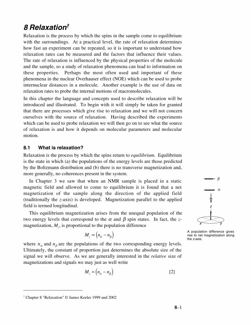
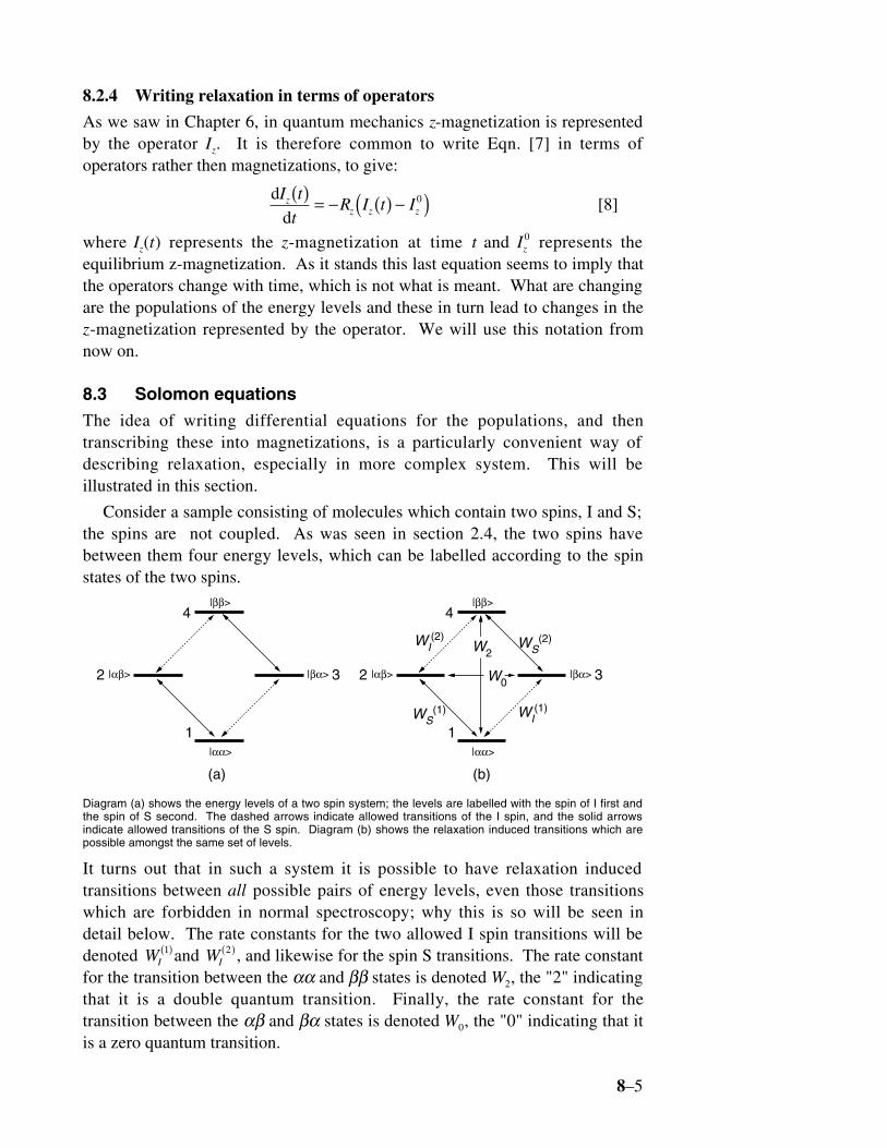
Consider a sample consisting of molecules which contain two spins, I and S;the spins are not coupled. As was seen in section 2.4, the two spins havebetween them four energy levels, which can be labelled according to the spinstates of the two spins.
|αα>
|ββ>
|αβ> |βα>
1
32
4
WI(1)
WI(2)
WS(1)
WS(2)
W2
W0
|αα>
|ββ>
|αβ> |βα>
1
32
4
(a) (b)
Diagram (a) shows the energy levels of a two spin system; the levels are labelled with the spin of I first andthe spin of S second. The dashed arrows indicate allowed transitions of the I spin, and the solid arrowsindicate allowed transitions of the S spin. Diagram (b) shows the relaxation induced transitions which arepossible amongst the same set of levels.
It turns out that in such a system it is possible to have relaxation inducedtransitions between all possible pairs of energy levels, even those transitionswhich are forbidden in normal spectroscopy; why this is so will be seen indetail below. The rate constants for the two allowed I spin transitions will bedenoted WI
1( )and WI2( ) , and likewise for the spin S transitions. The rate constant
for the transition between the αα and ββ states is denoted W2, the "2" indicatingthat it is a double quantum transition. Finally, the rate constant for thetransition between the αβ and βα states is denoted W0, the "0" indicating that itis a zero quantum transition.
8–6
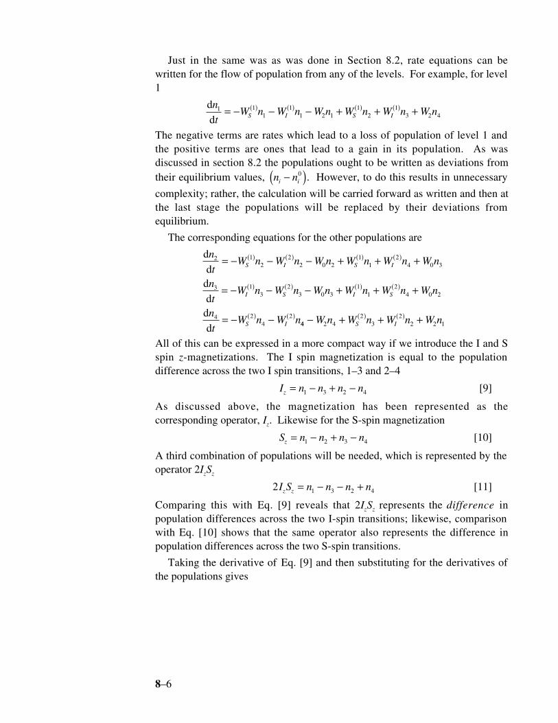
Just in the same was as was done in Section 8.2, rate equations can bewritten for the flow of population from any of the levels. For example, for level1
ddn
tW n W n W n W n W n W nS I S I
1 11
11 2 1
12
13 2 4= − − − + + +( ) ( ) ( ) ( )
The negative terms are rates which lead to a loss of population of level 1 andthe positive terms are ones that lead to a gain in its population. As wasdiscussed in section 8.2 the populations ought to be written as deviations fromtheir equilibrium values, n ni i−( )0 . However, to do this results in unnecessary
complexity; rather, the calculation will be carried forward as written and then atthe last stage the populations will be replaced by their deviations fromequilibrium.
The corresponding equations for the other populations are
dd
dd
dd
n
tW n W n W n W n W n W n
n
tW n W n W n W n W n W n
n
tW n W n
S I S I
I S I S
S I
2 12
22 0 2
11
24 0 3
3 13
23 0 3
11
24 0 2
4 24
2
= − − − + + +
= − − − + + +
= − −
( ) ( ) ( ) ( )
( ) ( ) ( ) ( )
( ) ( )44 2 4
23
22 2 1− + + +( ) ( )W n W n W n W nS I
All of this can be expressed in a more compact way if we introduce the I and Sspin z-magnetizations. The I spin magnetization is equal to the populationdifference across the two I spin transitions, 1–3 and 2–4
I n n n nz = − + −1 3 2 4 [9]
As discussed above, the magnetization has been represented as thecorresponding operator, Iz. Likewise for the S-spin magnetization
S n n n nz = − + −1 2 3 4 [10]
A third combination of populations will be needed, which is represented by theoperator 2IzSz
2 1 3 2 4I S n n n nz z = − − + [11]
Comparing this with Eq. [9] reveals that 2IzSz represents the difference inpopulation differences across the two I-spin transitions; likewise, comparisonwith Eq. [10] shows that the same operator also represents the difference inpopulation differences across the two S-spin transitions.
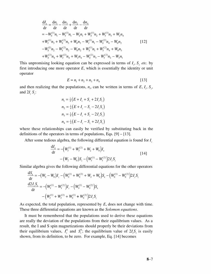
Taking the derivative of Eq. [9] and then substituting for the derivatives ofthe populations gives
8–7
dd
dd
dd
dd
dd
zI
t
n
t
n
t
n
t
n
t
W n W n W n W n W n W n
W n W n W n W n W n W n
W
S I S I
I S I S
S
= − + −
= − − − + + +
+ + + − − −
−
( ) ( ) ( ) ( )
( ) ( ) ( ) ( )
1 3 2 4
11
11 2 1
12
13 2 4
13
23 0 3
11
24 0 2
112
22 0 2
11
24 0 3
24
24 2 4
23
22 2 1
( ) ( ) ( ) ( )
( ) ( ) ( ) ( )
− − + + +
+ + + − − −
n W n W n W n W n W n
W n W n W n W n W n W n
I S I
S I S I
[12]
This unpromising looking equation can be expressed in terms of Iz, Sz etc. byfirst introducing one more operator E, which is essentially the identity or unitoperator
E n n n n= + + +1 2 3 4 [13]
and then realizing that the populations, ni, can be written in terms of E, Iz, Sz,and 2Iz Sz:
n E I S I S
n E I S I S
n E I S I S
n E I S I S
z z z z
z z z z
z z z z
z z z z
114
214
314
414
2
2
2
2
= + + +( )= + − −( )= − + −( )= − − +( )
where these relationships can easily be verified by substituting back in thedefinitions of the operators in terms of populations, Eqs. [9] – [13].
After some tedious algebra, the following differential equation is found for Iz
dd
zz
I
tW W W W I
W W S W W I S
I I
z I I z z
= − + + +( )− −( ) − −( )
( ) ( )
( ) ( )
1 22 0
2 01 2 2
[14]
Similar algebra gives the following differential equations for the other operators
dd
d2d
zz
zz
S
tW W I W W W W S W W I S
I S
tW W I W W S
W W W
z S S S S z z
zI I z S S
I I S
= − −( ) − + + +( ) − −( )= − −( ) − −( )
− + +
( ) ( ) ( ) ( )
( ) ( ) ( ) ( )
( ) ( ) ( )
2 01 2
2 01 2
1 2 1 2
1 2 1
2
++( )( )W I SS z z2 2
As expected, the total population, represented by E, does not change with time.These three differential equations are known as the Solomon equations.
It must be remembered that the populations used to derive these equationsare really the deviation of the populations from their equilibrium values. As aresult, the I and S spin magnetizations should properly be their deviations fromtheir equilibrium values, Iz
0 and Sz0; the equilibrium value of 2IzSz is easily
shown, from its definition, to be zero. For example, Eq. [14] becomes
8–8
d
d
zz
z
I I
tW W W W I I
W W S S W W I S
zI I z
z I I z z
−( )= − + + +( ) −( )
− −( ) −( ) − −( )
( ) ( )
( ) ( )
01 2
2 00
2 00 1 2 2
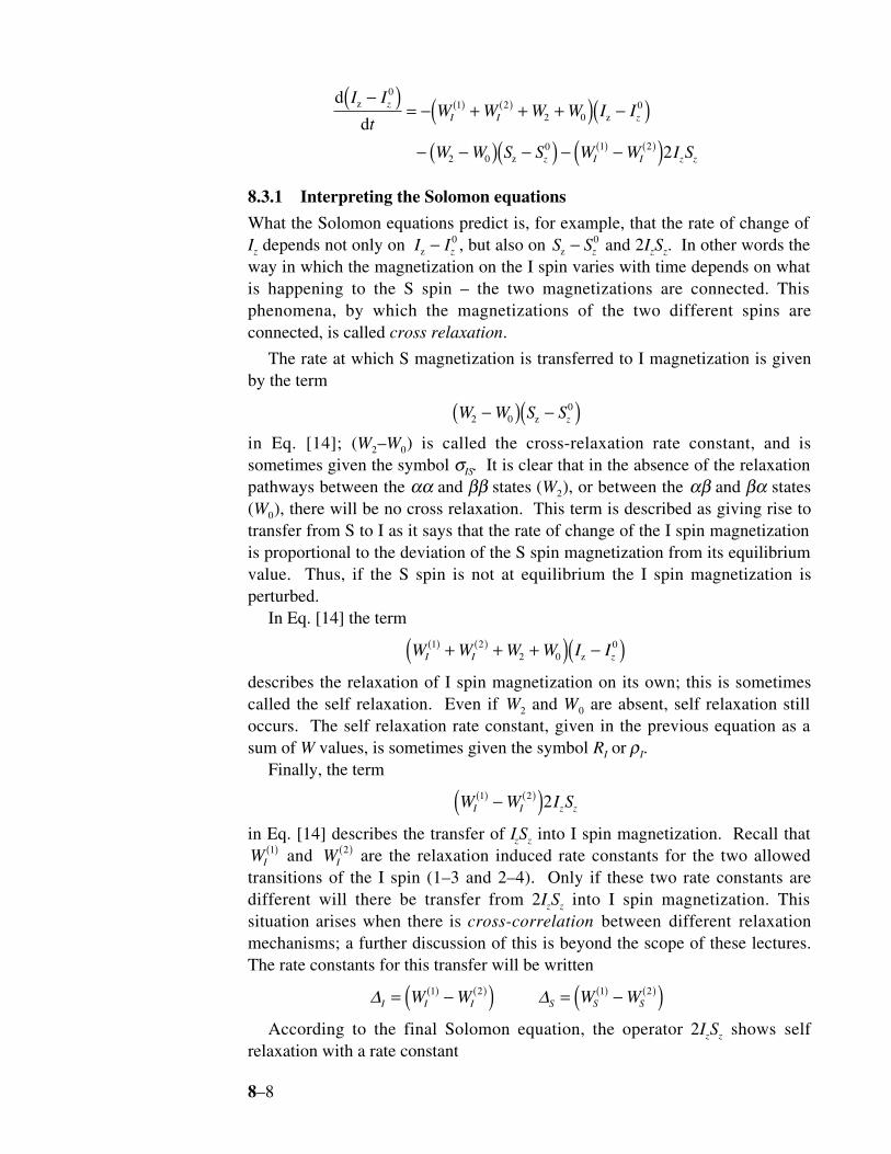
8.3.1 Interpreting the Solomon equations
What the Solomon equations predict is, for example, that the rate of change ofIz depends not only on I Izz − 0 , but also on S Szz − 0 and 2IzSz. In other words theway in which the magnetization on the I spin varies with time depends on whatis happening to the S spin – the two magnetizations are connected. Thisphenomena, by which the magnetizations of the two different spins areconnected, is called cross relaxation.
The rate at which S magnetization is transferred to I magnetization is givenby the term
W W S Sz2 00−( ) −( )z
in Eq. [14]; (W2–W0) is called the cross-relaxation rate constant, and issometimes given the symbol σIS. It is clear that in the absence of the relaxationpathways between the αα and ββ states (W2), or between the αβ and βα states(W0), there will be no cross relaxation. This term is described as giving rise totransfer from S to I as it says that the rate of change of the I spin magnetizationis proportional to the deviation of the S spin magnetization from its equilibriumvalue. Thus, if the S spin is not at equilibrium the I spin magnetization isperturbed.
In Eq. [14] the term
W W W W I II I z1 2
2 00( ) ( )+ + +( ) −( )z
describes the relaxation of I spin magnetization on its own; this is sometimescalled the self relaxation. Even if W2 and W0 are absent, self relaxation stilloccurs. The self relaxation rate constant, given in the previous equation as asum of W values, is sometimes given the symbol RI or ρI.
Finally, the term
W W I SI I z z1 2 2( ) ( )−( )
in Eq. [14] describes the transfer of IzSz into I spin magnetization. Recall thatWI
1( ) and WI2( ) are the relaxation induced rate constants for the two allowed
transitions of the I spin (1–3 and 2–4). Only if these two rate constants aredifferent will there be transfer from 2IzSz into I spin magnetization. Thissituation arises when there is cross-correlation between different relaxationmechanisms; a further discussion of this is beyond the scope of these lectures.The rate constants for this transfer will be written
∆ ∆I I I S S SW W W W= −( ) = −( )( ) ( ) ( ) ( )1 2 1 2
According to the final Solomon equation, the operator 2IzSz shows selfrelaxation with a rate constant
8–9
R W W W WIS I I S S= + + +( )( ) ( ) ( ) ( )1 2 1 2
Note that the W2 and W0 pathways do not contribute to this. This rate combinedconstant will be denoted RIS.
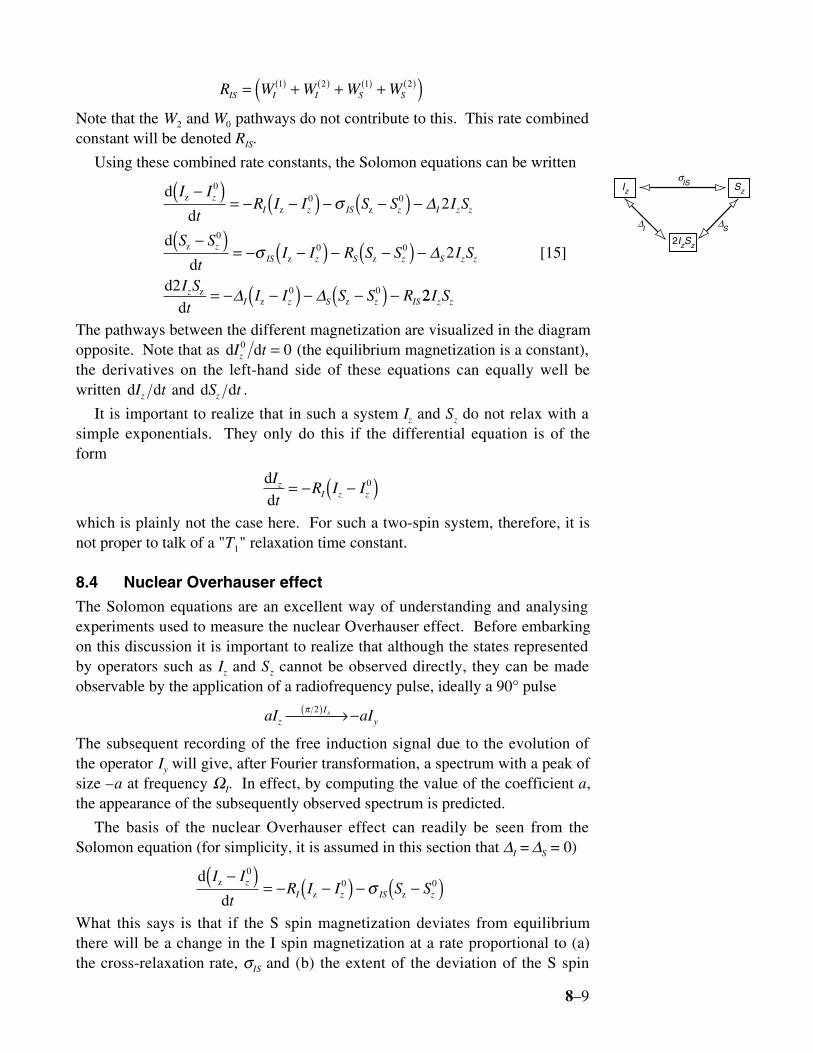
Using these combined rate constants, the Solomon equations can be written
d
d
d
dd2
d
zz z
zz z
zz z
I I
tR I I S S I S
S S
tI I R S S I S
I S
tI I S S R
zI z IS z I z z
zIS z S z S z z
zI z S z IS
−( )= − −( ) − −( ) −
−( )= − −( ) − −( ) −
= − −( ) − −( ) −
00 0
00 0
0 0
2
2
σ
σ
∆
∆
∆ ∆ 22I Sz z
[15]
The pathways between the different magnetization are visualized in the diagramopposite. Note that as d dI tz
0 0= (the equilibrium magnetization is a constant),the derivatives on the left-hand side of these equations can equally well bewritten d dI tz and d dS tz .
It is important to realize that in such a system Iz and Sz do not relax with asimple exponentials. They only do this if the differential equation is of theform
ddI
tR I Iz
I z z= − −( )0
which is plainly not the case here. For such a two-spin system, therefore, it isnot proper to talk of a "T1" relaxation time constant.
8.4 Nuclear Overhauser effect
The Solomon equations are an excellent way of understanding and analysingexperiments used to measure the nuclear Overhauser effect. Before embarkingon this discussion it is important to realize that although the states representedby operators such as Iz and Sz cannot be observed directly, they can be madeobservable by the application of a radiofrequency pulse, ideally a 90° pulse
aI aIzI
yxπ 2( ) → −
The subsequent recording of the free induction signal due to the evolution ofthe operator Iy will give, after Fourier transformation, a spectrum with a peak ofsize –a at frequency ΩI. In effect, by computing the value of the coefficient a,the appearance of the subsequently observed spectrum is predicted.
The basis of the nuclear Overhauser effect can readily be seen from theSolomon equation (for simplicity, it is assumed in this section that ∆I = ∆S = 0)
d
dz
z z
I I
tR I I S Sz
I z IS z
−( )= − −( ) − −( )
00 0σ
What this says is that if the S spin magnetization deviates from equilibriumthere will be a change in the I spin magnetization at a rate proportional to (a)the cross-relaxation rate, σIS and (b) the extent of the deviation of the S spin
σIS
∆I
∆S
2IzSz
Iz Sz
8–10
from equilibrium. This change in the I spin magnetization will manifest itselfas a change in the intensity in the corresponding spectrum, and it is this changein intensity of the I spin when the S spin is perturbed which is termed thenuclear Overhauser effect.
Plainly, there will be no such effect unless σIS is non-zero, which requires thepresence of the W2 and W0 relaxation pathways. It will be seen later on thatsuch pathways are only present when there is dipolar relaxation between thetwo spins and that the resulting cross-relaxation rate constants have a strongdependence on the distance between the two spins. The observation of anuclear Overhauser effect is therefore diagnostic of dipolar relaxation andhence the proximity of pairs of spins. The effect is of enormous value,therefore, in structure determination by NMR.
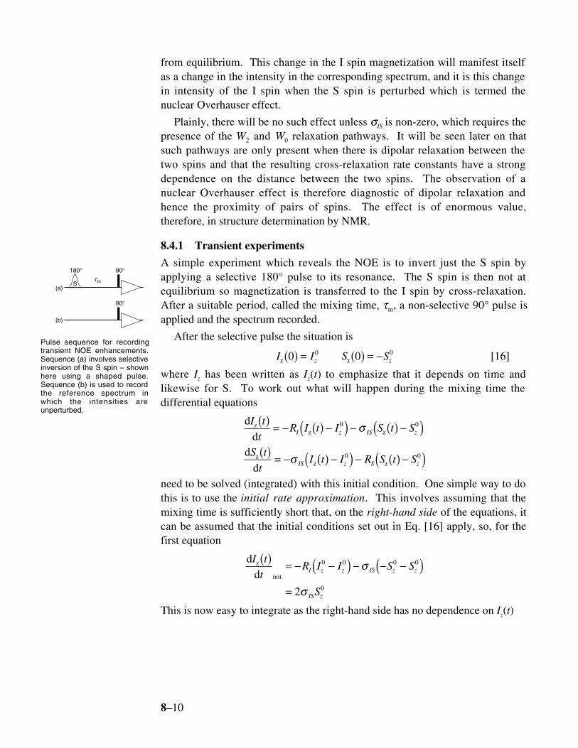
8.4.1 Transient experiments
A simple experiment which reveals the NOE is to invert just the S spin byapplying a selective 180° pulse to its resonance. The S spin is then not atequilibrium so magnetization is transferred to the I spin by cross-relaxation.After a suitable period, called the mixing time, τm, a non-selective 90° pulse isapplied and the spectrum recorded.
After the selective pulse the situation is
I I S Sz zz z0 00 0( ) = ( ) = − [16]
where Iz has been written as Iz(t) to emphasize that it depends on time andlikewise for S. To work out what will happen during the mixing time thedifferential equations
dd
dd
zz z
zz z
I t
tR I t I S t S
S t
tI t I R S t S
I z IS z
IS z S z
( ) = − ( ) −( ) − ( ) −( )( ) = − ( ) −( ) − ( ) −( )
0 0
0 0
σ
σ
need to be solved (integrated) with this initial condition. One simple way to dothis is to use the initial rate approximation. This involves assuming that themixing time is sufficiently short that, on the right-hand side of the equations, itcan be assumed that the initial conditions set out in Eq. [16] apply, so, for thefirst equation
ddz
init
I t
tR I I S S
S
I z z IS z z
IS z
( ) = − −( ) − − −( )=
0 0 0 0
02
σ
σThis is now easy to integrate as the right-hand side has no dependence on Iz(t)
mτ90°180°
S
90°
(a)
(b)
Pulse sequence for recordingtransient NOE enhancements.Sequence (a) involves selectiveinversion of the S spin – shownhere using a shaped pulse.Sequence (b) is used to recordthe reference spectrum inwhich the intensities areunperturbed.
8–11
d dz
z m z m
z m m
m m
I t S t
I I S
I S I
IS z
IS z
IS z z
( ) =
( ) − ( ) =
( ) = +
∫ ∫0
0
0
0
0 0
2
0 2
2
τ τ
σ
τ σ τ
τ σ τ
This says that for zero mixing time the I magnetization is equal to itsequilibrium value, but that as the mixing time increases the I magnetization hasan additional contribution which is proportional to the mixing time and thecross-relaxation rate, σIS. This latter term results in a change in the intensity ofthe I spin signal, and this change is called an NOE enhancement.
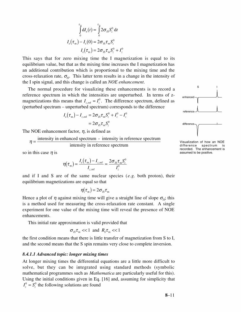
The normal procedure for visualizing these enhancements is to record areference spectrum in which the intensities are unperturbed. In terms of z-magnetizations this means that I Iz z, ref = 0 . The difference spectrum, defined as(perturbed spectrum – unperturbed spectrum) corresponds to the difference
I I S I I
S
z IS z z z
IS z
z m ref m
m
τ σ τ
σ τ
( ) − = + −
=, 2
2
0 0 0
0
The NOE enhancement factor, η, is defined as
η = intensity in enhanced spectrum - intensity in reference spectrumintensity in reference spectrum
so in this case η is
η ττ σ τ
mz m ref
ref
m( ) = ( ) −=
I I
I
S
Iz
z
IS z
z
,
,
2 0
0
and if I and S are of the same nuclear species (e.g. both proton), theirequilibrium magnetizations are equal so that
η τ σ τm m( ) = 2 IS
Hence a plot of η against mixing time will give a straight line of slope σIS; thisis a method used for measuring the cross-relaxation rate constant. A singleexperiment for one value of the mixing time will reveal the presence of NOEenhancements.
This initial rate approximation is valid provided that
σ τ τIS SRm m and << <<1 1
the first condition means that there is little transfer of magnetization from S to I,and the second means that the S spin remains very close to complete inversion.
8.4.1.1 Advanced topic: longer mixing times
At longer mixing times the differential equations are a little more difficult tosolve, but they can be integrated using standard methods (symbolicmathematical programmes such as Mathematica are particularly useful for this).Using the initial conditions given in Eq. [16] and, assuming for simplicity thatI Sz z
0 0= the following solutions are found
enhanced
reference
difference
S I
Visualization of how an NOEdi f ference spectrum isrecorded. The enhancement isassumed to be positive.
8–12
I
I Rz
z
ISτ σ λ τ λ τmm m
( ) = −( ) − −( )[ ] +0 2 1
21exp exp
S
I
R R
Rz
z
I Sτλ τ λ τ
λ τ λ τ
mm m
m m
( ) = −
−( ) − −( )[ ]+ − −( ) + −( )
0 1 2
1 21
exp exp
exp exp
where
R R R R R
R R R R R R
I I S S IS
I S I S
= − + +
= + +[ ] = + −[ ]
2 2 2
112 2
12
2 4σ
λ λ
These definitions ensure that λ1 > λ2. If RI and RS are not too dissimilar, R is ofthe order of σIS, and so the two rate constants λ1 and λ2 differ by a quantity ofthe order of σIS.
As expected for these two coupled differential equations, integration gives atime dependence which is the sum of two exponentials with different timeconstants.
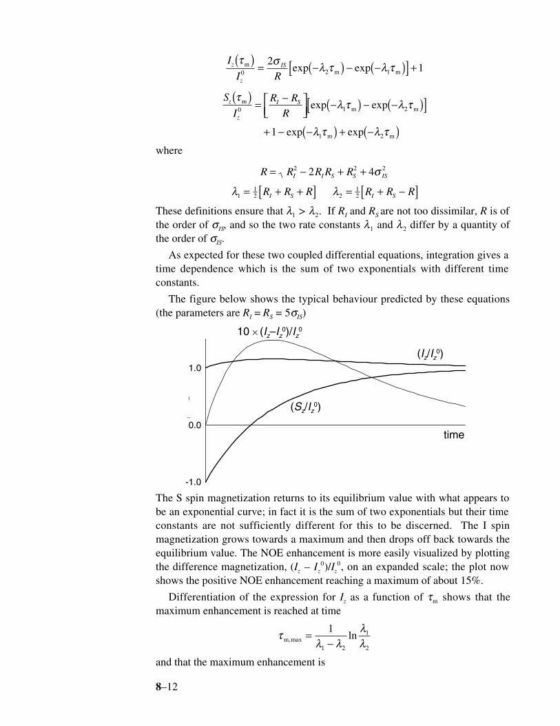
The figure below shows the typical behaviour predicted by these equations(the parameters are RI = RS = 5σIS)
0
-1.0
-0.5
0.0
0.5
1.0
1.5
time
(Sz/Iz0)
10 × (Iz–Iz0)/Iz
0
(Iz/Iz0)
The S spin magnetization returns to its equilibrium value with what appears tobe an exponential curve; in fact it is the sum of two exponentials but their timeconstants are not sufficiently different for this to be discerned. The I spinmagnetization grows towards a maximum and then drops off back towards theequilibrium value. The NOE enhancement is more easily visualized by plottingthe difference magnetization, (Iz – Iz
0)/Iz0, on an expanded scale; the plot now
shows the positive NOE enhancement reaching a maximum of about 15%.
Differentiation of the expression for Iz as a function of τm shows that themaximum enhancement is reached at time
τλ λ
λλm,max =
−1
1 2
1
2
ln
and that the maximum enhancement is
8–13
I I
I Rz z
z
ISR Rτ σ λ
λλλ
λ λ
m,max( ) −=
−
− −0
01
2
1
2
21 2
8.4.2 The DPFGSE NOE experiment
From the point of view of the relaxation behaviour the DPFGSE experiment isessentially identical to the transient NOE experiment. The only difference isthat the I spin starts out saturated rather than at equilibrium. This does notinfluence the build up of the NOE enhancement on I. It does, however, havethe advantage of reducing the size of the I spin signal which has to be removedin the difference experiment. Further discussion of this experiment is deferredto Chapter 9.
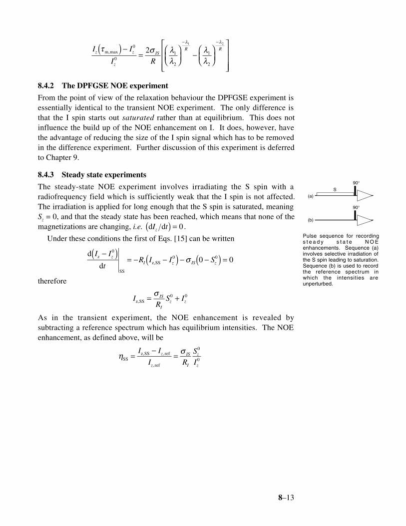
8.4.3 Steady state experiments
The steady-state NOE experiment involves irradiating the S spin with aradiofrequency field which is sufficiently weak that the I spin is not affected.The irradiation is applied for long enough that the S spin is saturated, meaningSz = 0, and that the steady state has been reached, which means that none of themagnetizations are changing, i.e. d dI tz( ) = 0 .
Under these conditions the first of Eqs. [15] can be written
d
dz
SS
z,SS
I I
tR I I Sz
I z IS z
−( )= − −( ) − −( ) =
00 00 0σ
therefore
IR
S IIS
Iz zz,SS = +σ 0 0
As in the transient experiment, the NOE enhancement is revealed bysubtracting a reference spectrum which has equilibrium intensities. The NOEenhancement, as defined above, will be
η σSS
z,SS ref
ref
=−
=I I
I R
S
Iz
z
IS
I
z
z
,
,
0
0
90°S
90°
(a)
(b)
Pulse sequence for recordings t e a d y s t a t e N O Eenhancements. Sequence (a)involves selective irradiation ofthe S spin leading to saturation.Sequence (b) is used to recordthe reference spectrum inwhich the intensities areunperturbed.
8–14
In contrast to the transient experiment, the steady state enhancement onlydepends on the relaxation of the receiving spin (here I); the relaxation rate ofthe S spin does not enter into the relationship simply because this spin is heldsaturated during the experiment.
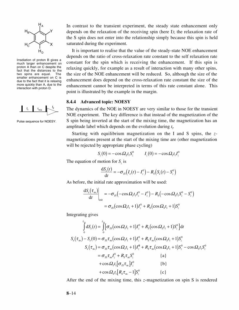
It is important to realise that the value of the steady-state NOE enhancementdepends on the ratio of cross-relaxation rate constant to the self relaxation rateconstant for the spin which is receiving the enhancement. If this spin isrelaxing quickly, for example as a result of interaction with many other spins,the size of the NOE enhancement will be reduced. So, although the size of theenhancement does depend on the cross-relaxation rate constant the size of theenhancement cannot be interpreted in terms of this rate constant alone. Thispoint is illustrated by the example in the margin.
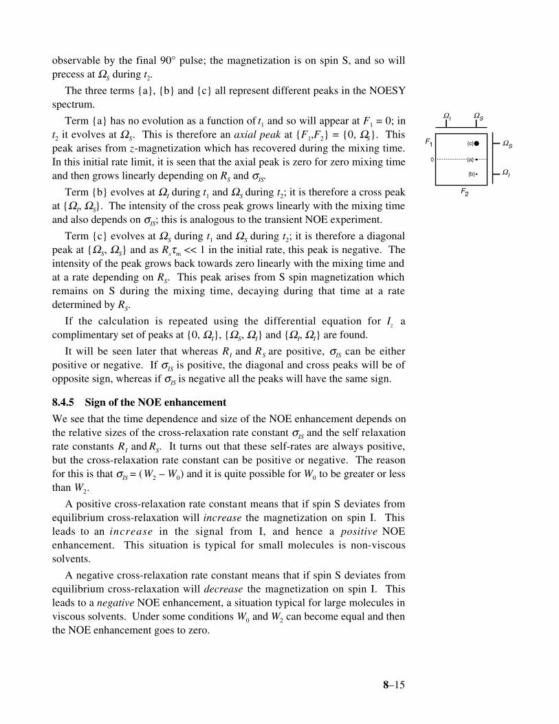
8.4.4 Advanced topic: NOESY
The dynamics of the NOE in NOESY are very similar to those for the transientNOE experiment. The key difference is that instead of the magnetization of theS spin being inverted at the start of the mixing time, the magnetization has anamplitude label which depends on the evolution during tl.
Starting with equilibrium magnetization on the I and S spins, the z-magnetizations present at the start of the mixing time are (other magnetizationwill be rejected by appropriate phase cycling)
S t S I t Iz S z z I z0 010
10( ) = − ( ) = −cos cosΩ Ω
The equation of motion for Sz is
ddz
z z
S t
tI t I R S t SIS z S z
( ) = − ( ) −( ) − ( ) −( )σ 0 0
As before, the initial rate approximation will be used:
d
dz m
init
S
tt I I R t S S
t I R t S
IS I z z S S z z
IS I z S S z
τσ
σ
( ) = − − −( ) − − −( )= +( ) + +( )
cos cos
cos cos
Ω Ω
Ω Ω
10 0
10 0
10
101 1
Integrating gives
d dz
z m z m m
z m m
m m
S t t I R t S t
S S t I R t S
S t I
IS I z S S z
IS I z S S z
IS I z
( ) = +( ) + +( )[ ]( ) − ( ) = +( ) + +( )
( ) = +( )
∫ ∫0
10
10
0
10
10
1
1 1
0 1 1
1
τ τ
σ
τ σ τ τ
τ σ τ
cos cos
cos cos
cos
Ω Ω
Ω Ω
Ω 001
01
0
0 0
10
10
1
1
+ +( ) −
= +
+ [ ]+ −[ ]
R t S t S
I R S
t I
t R S
S S z S z
IS z S z
I IS z
S S z
τ
σ τ τ
σ τ
τ
m
m m
m
m
a
b
c
cos cos
cos
cos
Ω Ω
Ω
Ω
After the end of the mixing time, this z-magnetization on spin S is rendered
HA
HB
HC
HD
X
Y
Irradiation of proton B gives amuch larger enhancement onproton A than on C despite thefact that the distances to thetwo spins are equal. Thesmaller enhancement on C isdue to the fact that it is relaxingmore quickly than A, due to theinteraction with proton D.
t1t2τmix
Pulse sequence for NOESY.
8–15
observable by the final 90° pulse; the magnetization is on spin S, and so willprecess at ΩS during t2.
The three terms a, b and c all represent different peaks in the NOESYspectrum.
Term a has no evolution as a function of t1 and so will appear at F1 = 0; int2 it evolves at ΩS. This is therefore an axial peak at F1,F2 = 0, ΩS. Thispeak arises from z-magnetization which has recovered during the mixing time.In this initial rate limit, it is seen that the axial peak is zero for zero mixing timeand then grows linearly depending on RS and σIS.
Term b evolves at ΩI during t1 and ΩS during t2; it is therefore a cross peakat ΩI, ΩS. The intensity of the cross peak grows linearly with the mixing timeand also depends on σIS; this is analogous to the transient NOE experiment.
Term c evolves at ΩS during t1 and ΩS during t2; it is therefore a diagonalpeak at ΩS, ΩS and as Rsτm << 1 in the initial rate, this peak is negative. Theintensity of the peak grows back towards zero linearly with the mixing time andat a rate depending on RS. This peak arises from S spin magnetization whichremains on S during the mixing time, decaying during that time at a ratedetermined by RS.
If the calculation is repeated using the differential equation for Iz acomplimentary set of peaks at 0, ΩI, ΩS, ΩI and ΩI, ΩI are found.
It will be seen later that whereas RI and RS are positive, σIS can be eitherpositive or negative. If σIS is positive, the diagonal and cross peaks will be ofopposite sign, whereas if σIS is negative all the peaks will have the same sign.
8.4.5 Sign of the NOE enhancement
We see that the time dependence and size of the NOE enhancement depends onthe relative sizes of the cross-relaxation rate constant σIS and the self relaxationrate constants RI and RS. It turns out that these self-rates are always positive,but the cross-relaxation rate constant can be positive or negative. The reasonfor this is that σIS = (W2 – W0) and it is quite possible for W0 to be greater or lessthan W2.
A positive cross-relaxation rate constant means that if spin S deviates fromequilibrium cross-relaxation will increase the magnetization on spin I. Thisleads to an increase in the signal from I, and hence a positive NOEenhancement. This situation is typical for small molecules is non-viscoussolvents.
A negative cross-relaxation rate constant means that if spin S deviates fromequilibrium cross-relaxation will decrease the magnetization on spin I. Thisleads to a negative NOE enhancement, a situation typical for large molecules inviscous solvents. Under some conditions W0 and W2 can become equal and thenthe NOE enhancement goes to zero.
IΩ
IΩ
SΩ
SΩF1
F2
a
b
c
0
8–16
8.5 Origins of relaxation
We now turn to the question as to what causes relaxation. Recall from section8.1 that relaxation involves transitions between energy levels, so what we seekis the origin of these transitions. We already know from Chapter 3 thattransitions are caused by transverse magnetic fields (i.e. in the xy-plane) whichare oscillating close to the Larmor frequency. An RF pulse gives rise to justsuch a field.
However, there is an important distinction between the kind of transitionscaused by RF pulses and those which lead to relaxation. When an RF pulse isapplied all of the spins experience the same oscillating field. The kind oftransitions which lead to relaxation are different in that the transverse fields arelocal, meaning that they only affect a few spins and not the whole sample. Inaddition, these fields vary randomly in direction and amplitude. In fact, it isprecisely their random nature which drives the sample to equilibrium.
The fields which are responsible for relaxation are generated within thesample, often due to interactions of spins with one another or with theirenvironment in some way. They are made time varying by the random motions(rotations, in particular) which result from the thermal agitation of themolecules and the collisions between them. Thus we will see that NMRrelaxation rate constants are particularly sensitive to molecular motion.
If the spins need to lose energy to return to equilibrium they give this up tothe motion of the molecules. Of course, the amounts of energy given up by thespins are tiny compared to the kinetic energies that molecules have, so they arehardly affected. Likewise, if the spins need to increase their energy to go toequilibrium, for example if the population of the β state has to be increased, thisenergy comes from the motion of the molecules.
Relaxation is essentially the process by which energy is allowed to flowbetween the spins and molecular motion. This is the origin of the original namefor longitudinal relaxation: spin-lattice relaxation. The lattice does not refer toa solid, but to the motion of the molecules with which energy can beexchanged.
8.5.1 Factors influencing the relaxation rate constant
The detailed theory of the calculation of relaxation rate constants is beyond thescope of this course. However, we are in a position to discuss the kinds offactors which influence these rate constants.
Let us consider the rate constant Wij for transitions between levels i and j;this turns out to depend on three factors:
W A Y Jij ij ij= × × ( )ω
We will consider each in turn.
The spin factor, Aij
This factor depends on the quantum mechanical details of the interaction. For
8–17
example, not all oscillating fields can cause transitions between all levels. In atwo spin system the transition between the αα and ββ cannot be brought aboutby a simple oscillating field in the transverse plane; in fact it needs a morecomplex interaction that is only present in the dipolar mechanism (section8.6.2). We can think of Aij as representing a kind of selection rule for theprocess – like a selection rule it may be zero for some transitions.
The size factor, Y
This is just a measure of how large the interaction causing the relaxation is. Itssize depends on the detailed origin of the random fields and often it is related tomolecular geometry.
The spectral density, J(ω ij)
This is a measure of the amount of molecular motion which is at the correctfrequency, ωij, to cause the transitions. Recall that molecular motion is theeffect which makes the random fields vary with time. However, as we sawwith RF pulses, the field will only have an effect on the spins if it is oscillatingat the correct frequency. The spectral density is a measure of how much of themotion is present at the correct frequency.
8.5.2 Spectral densities and correlation functions
The value of the spectral density, J(ω), has a large effect on relaxation rateconstants, so it is well worthwhile spending some time in understanding theform that this function takes.
Correlation functions
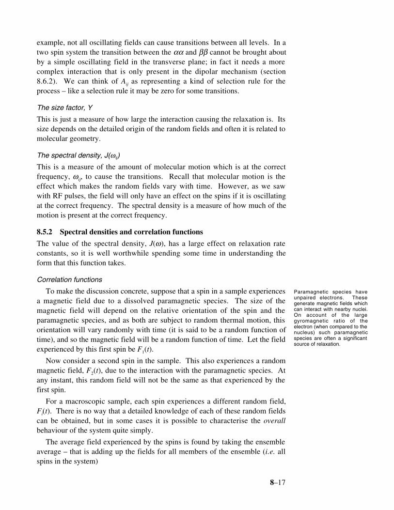
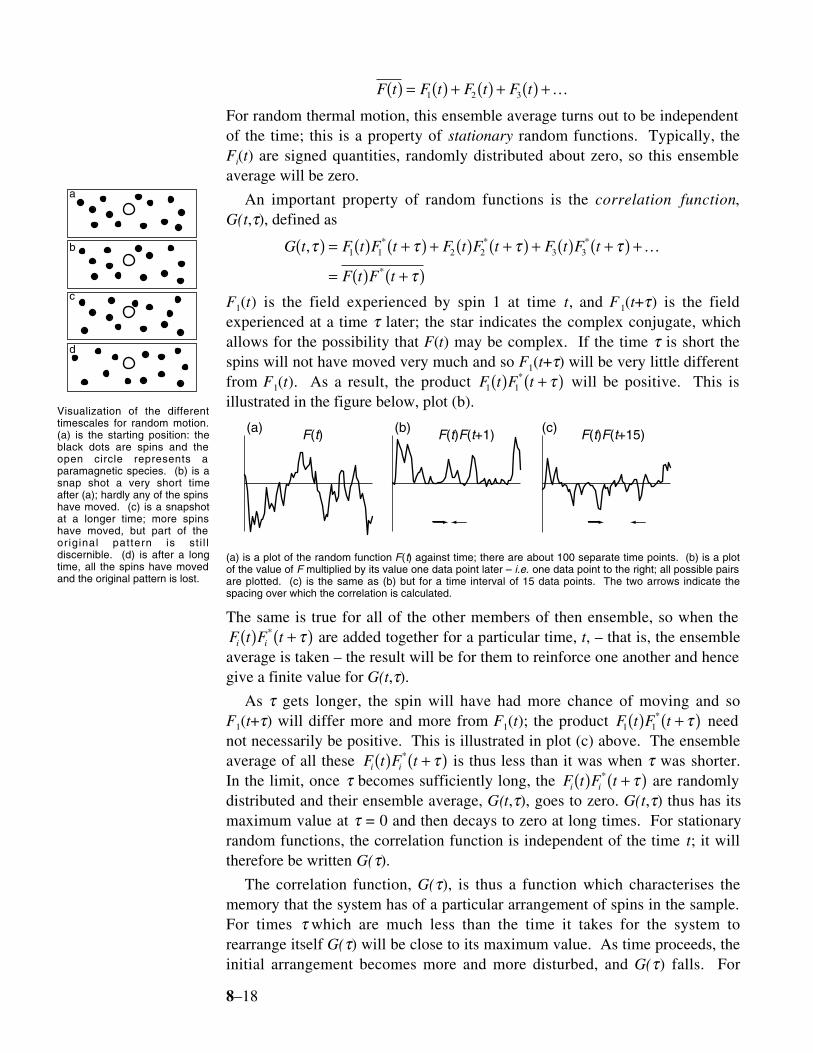
To make the discussion concrete, suppose that a spin in a sample experiencesa magnetic field due to a dissolved paramagnetic species. The size of themagnetic field will depend on the relative orientation of the spin and theparamagnetic species, and as both are subject to random thermal motion, thisorientation will vary randomly with time (it is said to be a random function oftime), and so the magnetic field will be a random function of time. Let the fieldexperienced by this first spin be F1(t).
Now consider a second spin in the sample. This also experiences a randommagnetic field, F2(t), due to the interaction with the paramagnetic species. Atany instant, this random field will not be the same as that experienced by thefirst spin.
For a macroscopic sample, each spin experiences a different random field,Fi(t). There is no way that a detailed knowledge of each of these random fieldscan be obtained, but in some cases it is possible to characterise the overallbehaviour of the system quite simply.
The average field experienced by the spins is found by taking the ensembleaverage – that is adding up the fields for all members of the ensemble (i.e. allspins in the system)
Paramagnetic species haveunpaired electrons. Thesegenerate magnetic fields whichcan interact with nearby nuclei.On account of the largegyromagnetic ratio of theelectron (when compared to thenucleus) such paramagneticspecies are often a significantsource of relaxation.
8–18
F t F t F t F t( ) = ( ) + ( ) + ( ) +1 2 3 K
For random thermal motion, this ensemble average turns out to be independentof the time; this is a property of stationary random functions. Typically, theFi(t) are signed quantities, randomly distributed about zero, so this ensembleaverage will be zero.
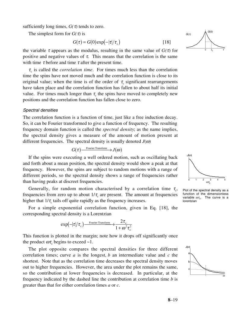
An important property of random functions is the correlation function,G(t,τ), defined as
G t F t F t F t F t F t F t
F t F t
, * * *
*
τ τ τ τ
τ
( ) = ( ) +( ) + ( ) +( ) + ( ) +( ) +
= ( ) +( )1 1 2 2 3 3 K
F1(t) is the field experienced by spin 1 at time t, and F 1(t+τ) is the fieldexperienced at a time τ later; the star indicates the complex conjugate, whichallows for the possibility that F(t) may be complex. If the time τ is short thespins will not have moved very much and so F1(t+τ) will be very little differentfrom F1(t). As a result, the product F t F t1 1( ) +( )* τ will be positive. This isillustrated in the figure below, plot (b).
5-1.2 5-1.2 5-1.2
F(t) F(t)F(t+1) F(t)F(t+15)(a) (b) (c)
(a) is a plot of the random function F(t) against time; there are about 100 separate time points. (b) is a plotof the value of F multiplied by its value one data point later – i.e. one data point to the right; all possible pairsare plotted. (c) is the same as (b) but for a time interval of 15 data points. The two arrows indicate thespacing over which the correlation is calculated.
The same is true for all of the other members of then ensemble, so when theF t F ti i( ) +( )* τ are added together for a particular time, t, – that is, the ensembleaverage is taken – the result will be for them to reinforce one another and hencegive a finite value for G(t,τ).
As τ gets longer, the spin will have had more chance of moving and soF1(t+τ) will differ more and more from F1(t); the product F t F t1 1( ) +( )* τ neednot necessarily be positive. This is illustrated in plot (c) above. The ensembleaverage of all these F t F ti i( ) +( )* τ is thus less than it was when τ was shorter.In the limit, once τ becomes sufficiently long, the F t F ti i( ) +( )* τ are randomlydistributed and their ensemble average, G(t,τ), goes to zero. G(t,τ) thus has itsmaximum value at τ = 0 and then decays to zero at long times. For stationaryrandom functions, the correlation function is independent of the time t; it willtherefore be written G(τ).
The correlation function, G(τ), is thus a function which characterises thememory that the system has of a particular arrangement of spins in the sample.For times τ which are much less than the time it takes for the system torearrange itself G(τ) will be close to its maximum value. As time proceeds, theinitial arrangement becomes more and more disturbed, and G(τ) falls. For
a
b
c
d
Visualization of the differenttimescales for random motion.(a) is the starting position: theblack dots are spins and theopen circle represents aparamagnetic species. (b) is asnap shot a very short timeafter (a); hardly any of the spinshave moved. (c) is a snapshotat a longer time; more spinshave moved, but part of theoriginal pattern is st i l ldiscernible. (d) is after a longtime, all the spins have movedand the original pattern is lost.
8–19
sufficiently long times, G(τ) tends to zero.
The simplest form for G(τ) is
G Gτ τ τ( ) = ( ) −( )0 exp c [18]
the variable τ appears as the modulus, resulting in the same value of G(τ) forpositive and negative values of τ. This means that the correlation is the samewith time τ before and time τ after the present time.
τc is called the correlation time. For times much less than the correlationtime the spins have not moved much and the correlation function is close to itsoriginal value; when the time is of the order of τc significant rearrangementshave taken place and the correlation function has fallen to about half its initialvalue. For times much longer than τc the spins have moved to completely newpositions and the correlation function has fallen close to zero.
Spectral densities
The correlation function is a function of time, just like a free induction decay.So, it can be Fourier transformed to give a function of frequency. The resultingfrequency domain function is called the spectral density; as the name implies,the spectral density gives a measure of the amount of motion present atdifferent frequencies. The spectral density is usually denoted J(ω)
G Jτ ω( ) → ( )Fourier Transform
If the spins were executing a well ordered motion, such as oscillating backand forth about a mean position, the spectral density would show a peak at thatfrequency. However, the spins are subject to random motions with a range ofdifferent periods, so the spectral density shows a range of frequencies ratherthan having peaks at discreet frequencies.
Generally, for random motion characterised by a correlation time τc,frequencies from zero up to about 1/τc are present. The amount at frequencieshigher that 1/τc tails off quite rapidly as the frequency increases.
For a simple exponential correlation function, given in Eq. [18], thecorresponding spectral density is a Lorentzian
exp −( ) →+
τ τ τω τc
Fourier Transform c
c2
21 2
This function is plotted in the margin; note how it drops off significantly oncethe product ωτc begins to exceed ~1.
The plot opposite compares the spectral densities for three differentcorrelation times; curve a is the longest, b an intermediate value and c theshortest. Note that as the correlation time decreases the spectral density movesout to higher frequencies. However, the area under the plot remains the same,so the contribution at lower frequencies is decreased. In particular, at thefrequency indicated by the dashed line the contribution at correlation time b isgreater than that for either correlation times a or c.
0
0
0
G( )G(0)
ττ
τ
c
0 1 2 3 4 50
J( )ω
ωτc
Plot of the spectral density as afunction of the dimensionlessvariable ωτc. The curve is alorentzian
00
J( )ω
ω
a
b
c
8–20
For this spectral density function, the maximum contribution at frequency ωis found when τc is 1/ω; this has important consequences which are described inthe next section.
8.5.3 The "T1 minimum"
In the case of relaxation of a single spin by a random field (such as thatgenerated by a paramagnetic species), the only relevant spectral density is thatat the Larmor frequency, ω0. This is hardly surprising as to cause relaxation –that is to cause transitions – the field needs to have components oscillating atthe Larmor frequency.
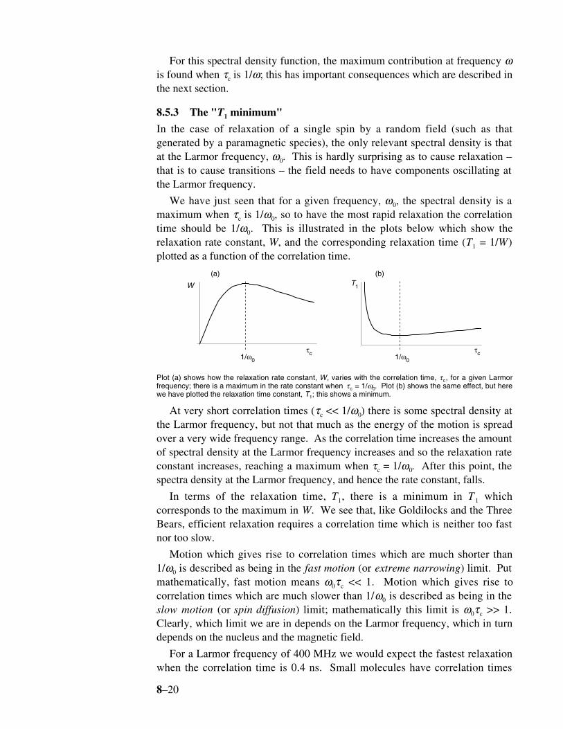
We have just seen that for a given frequency, ω0, the spectral density is amaximum when τc is 1/ω0, so to have the most rapid relaxation the correlationtime should be 1/ω0. This is illustrated in the plots below which show therelaxation rate constant, W, and the corresponding relaxation time (T1 = 1/W)plotted as a function of the correlation time.
τc1/ω0
τc
W T1
1/ω0
(a) (b)
Plot (a) shows how the relaxation rate constant, W, varies with the correlation time, τc, for a given Larmorfrequency; there is a maximum in the rate constant when τc = 1/ω0. Plot (b) shows the same effect, but herewe have plotted the relaxation time constant, T1; this shows a minimum.
At very short correlation times (τc << 1/ω0) there is some spectral density atthe Larmor frequency, but not that much as the energy of the motion is spreadover a very wide frequency range. As the correlation time increases the amountof spectral density at the Larmor frequency increases and so the relaxation rateconstant increases, reaching a maximum when τc = 1/ω0. After this point, thespectra density at the Larmor frequency, and hence the rate constant, falls.
In terms of the relaxation time, T1, there is a minimum in T 1 whichcorresponds to the maximum in W. We see that, like Goldilocks and the ThreeBears, efficient relaxation requires a correlation time which is neither too fastnor too slow.
Motion which gives rise to correlation times which are much shorter than1/ω0 is described as being in the fast motion (or extreme narrowing) limit. Putmathematically, fast motion means ω0τc << 1. Motion which gives rise tocorrelation times which are much slower than 1/ω0 is described as being in theslow motion (or spin diffusion) limit; mathematically this limit is ω0τc >> 1.Clearly, which limit we are in depends on the Larmor frequency, which in turndepends on the nucleus and the magnetic field.
For a Larmor frequency of 400 MHz we would expect the fastest relaxationwhen the correlation time is 0.4 ns. Small molecules have correlation times
8–21
significantly shorter than this (say tens of ps), so such molecules are clearly inthe fast motion limit. Large molecules, such as proteins, can easily havecorrelation times of the order of a few ns, and these clearly fall in the slowmotion limit.
Somewhat strangely, therefore, both very small and very large moleculestend to relax more slowly than medium-sized molecules.
8.6 Relaxation mechanisms
So far, the source of the magnetic fields which give rise to relaxation and theorigin of their time dependence have not been considered. Each such source isreferred to as a relaxation mechanism. There are quite a range of differentmechanisms that can act, but of these only a few are really important for spinhalf nuclei.
8.6.1 Paramagnetic species
We have already mentioned this source of varying fields several times. Thelarge magnetic moment of the electron means that paramagnetic species insolution are particularly effective at promoting relaxation. Such species includedissolved oxygen and certain transition metal compounds.
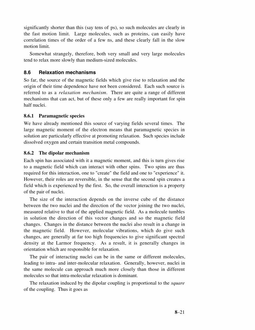
8.6.2 The dipolar mechanism
Each spin has associated with it a magnetic moment, and this is turn gives riseto a magnetic field which can interact with other spins. Two spins are thusrequired for this interaction, one to "create" the field and one to "experience" it.However, their roles are reversible, in the sense that the second spin creates afield which is experienced by the first. So, the overall interaction is a propertyof the pair of nuclei.
The size of the interaction depends on the inverse cube of the distancebetween the two nuclei and the direction of the vector joining the two nuclei,measured relative to that of the applied magnetic field. As a molecule tumblesin solution the direction of this vector changes and so the magnetic fieldchanges. Changes in the distance between the nuclei also result in a change inthe magnetic field. However, molecular vibrations, which do give suchchanges, are generally at far too high frequencies to give significant spectraldensity at the Larmor frequency. As a result, it is generally changes inorientation which are responsible for relaxation.
The pair of interacting nuclei can be in the same or different molecules,leading to intra- and inter-molecular relaxation. Generally, however, nuclei inthe same molecule can approach much more closely than those in differentmolecules so that intra-molecular relaxation is dominant.
The relaxation induced by the dipolar coupling is proportional to the squareof the coupling. Thus it goes as
8–22
γ γ12
22
126
1r
where γ1 and γ2 are the gyromagnetic ratios of the two nuclei involved and r12 isthe distance between them.
As the size of the dipolar interaction depends on the product of thegyromagnetic ratios of the two nuclei involved, and the resulting relaxation rateconstants depends on the square of this. Thus, pairs of nuclei with highgyromagnetic ratios are most efficient at promoting relaxation. For example,every thing else being equal, a proton-proton pair will relax 16 times faster thana carbon-13 proton pair.
It is important to realize that in dipolar relaxation the effect is not primarilyto distribute the energy from one of the spins to the other. This would not, onits own, bring the spins to equilibrium. Rather, the dipolar interaction providesa path by which energy can be transferred between the lattice and the spins. Inthis case, the lattice is the molecular motion. Essentially, the dipole-dipoleinteraction turns molecular motion into an oscillating magnetic field which cancause transitions of the spins.
Relation to the NOE
The dipolar mechanism is the only common relaxation mechanism which cancause transitions in which more than one spin flips. Specifically, with referenceto section 8.3, the dipolar mechanism gives rise to transitions between the ααand ββ states (W2) and between the αβ and βα states (W0).
The rate constant W2 corresponds to transitions which are at the sum of theLarmor frequencies of the two spins, (ω0,I + ω0,S) and so it is the spectral densityat this sum frequency which is relevant. In contrast, W0 corresponds totransitions at (ω0,I – ω 0,S) and so for these it is the spectral density at thisdifference frequency which is relevant.
In the case where the two spins are the same (e.g. two protons) the tworelevant spectral densities are J(2ω0) and J(0). In the fast motion limit (ω0τc <<1) J(2ω0) is somewhat less than J(0), but not by very much. A detailedcalculation shows that W2 > W 0 and so we expect to see positive NOEenhancements (section 8.4.5). In contrast, in the slow motion limit (ω0τc >> 1)J(2ω0) is all but zero and so J(0) >> J(2ω0); not surprisingly it follows that W0 >W2 and a negative NOE enhancement is seen.
8.6.3 The chemical shift anisotropy mechanism
The chemical shift arises because, due to the effect of the electrons in amolecule, the magnetic field experienced by a nucleus is different to thatapplied to the sample. In liquids, all that is observable is the average chemicalshift, which results from the molecule rapidly experiencing all possibleorientations by rapid molecular tumbling.
At a more detailed level, the magnetic field experienced by the nucleus
8–23
depends on the orientation of the molecule relative to the applied magneticfield. This is called chemical shift anisotropy (CSA). In addition, it is not onlythe magnitude of the field which is altered but also its direction. The changesare very small, but sufficient to be detectable in the spectrum and to give rise torelaxation.
One convenient way of imagining the effect of CSA is to say that due to itthere are small additional fields created at the nucleus – in general in all threedirections. These fields vary in size as the molecule reorients, and so they havethe necessary time variation to cause relaxation. As has already been discussed,it is the transverse fields which will give rise to changes in population.
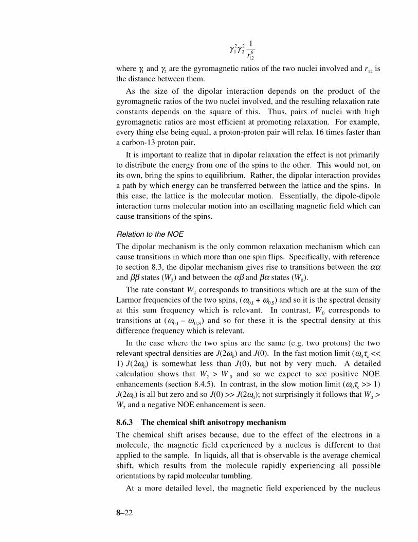
The size of the CSA is specified by a tensor, which is a mathematical objectrepresented by a three by three matrix.
σσ σ σσ σ σσ σ σ
=
xx xy xz
yx yy yz
zx zy zz
The element σxz gives the size of the extra field in the x-direction which resultsfrom a field being applied in the z-direction; likewise, σyz gives the extra field inthe y-direction and σzz that in the z-direction. These elements depend on theelectronic properties of the molecule and the orientation of the molecule withrespect to the magnetic field.
Detailed calculations show that the relaxation induced by CSA goes as thesquare of the field strength and is also proportional to the shift anisotropy. Arough estimate of the size of this anisotropy is that it is equal to the typical shiftrange. So, CSA relaxation is expected to be significant for nuclei with largeshift ranges observed at high fields. It is usually insignificant for protons.
8.7 Transverse relaxation
Right at the start of this section we mentioned that relaxation involved twoprocesses: the populations returning to equilibrium and the transversemagnetization decaying to zero. So far, we have only discussed the fist of thesetwo. The second, in which the transverse magnetization decays, is calledtransverse (or spin-spin) relaxation.
8–24
(a)
(b)
(c)
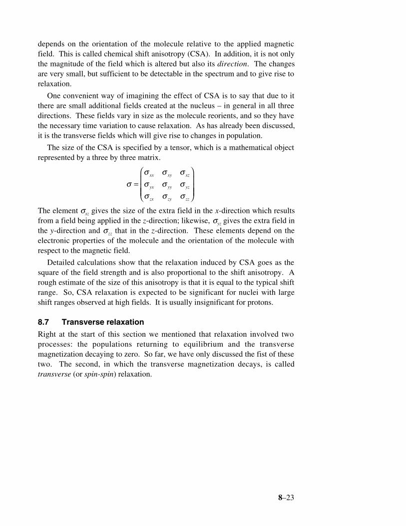
Depiction of how the individual contributions from different spins (shown on the left) add up to give the nettransverse magnetization (on the right). See text for details.
Each spin in the sample can be thought of as giving rise to a smallcontribution to the magnetization; these contributions can be in any direction,and in general have a component along x, y and z. The individual contributionsalong z add up to give the net z-magnetization of the sample.
The transverse contributions behave in a more complex way as, just like thenet transverse magnetization, these contributions are precessing at the Larmorfrequency in the transverse plane. We can represent each of these contributionsby a vector precessing in the transverse plane.
The direction in which these vectors point can be specified by giving each aphase – arbitrarily the angle measured around from the x -axis. It isimmediately clear that if these phases are random the net transversemagnetization of the sample will be zero as all the individual contributions willcancel. This is the situation that pertains at equilibrium and is shown in (a) inthe figure above.
For there to be net magnetization, the phases must not be random, ratherthere has to be a preference for one direction; this is shown in (b) in the figureabove. In quantum mechanics this is described as a coherence. An RF pulseapplied to equilibrium magnetization generates transverse magnetization, or inother words the pulse generates a coherence. Transverse relaxation destroysthis coherence by destroying the alignment of the individual contributions, as
8–25
shown in (c) above.
Our picture indicates that there are two ways in which the coherence couldbe destroyed. The first is to make the vectors jump to new positions, atrandom. Drawing on our analogy between these vectors and the behaviour ofthe bulk magnetization, we can see that these jumps could be brought about bylocal oscillating fields which have the same effect as pulses.
This is exactly what causes longitudinal relaxation, in which we imagine thelocal fields causing the spins to flip. So, anything that causes longitudinalrelaxation will also cause transverse relaxation.
The second way of destroying the coherence is to make the vectors get out ofstep with one another as a result of them precessing at different Larmorfrequencies. Again, a local field plays the part we need but this time we do notneed it to oscillate; rather, all we need for it to do is to be different at differentlocations in the sample.
This latter contribution is called the secular part of transverse relaxation; thepart which has the same origin as longitudinal relaxation is called the non-secular part.
It turns out that the secular part depends on the spectral density at zerofrequency, J(0). We can see that this makes sense as this part of transverserelaxation requires no transitions, just a field to cause a local variation in themagnetic field. Looking at the result from section 8.5.2 we see that J(0) = 2τc,and so as the correlation time gets longer and longer, so too does the relaxationrate constant. Thus large molecules in the slow motion limit are characterisedby very rapid transverse relaxation; this is in contrast to longitudinal relaxationis most rapid for a particular value of the correlation time.
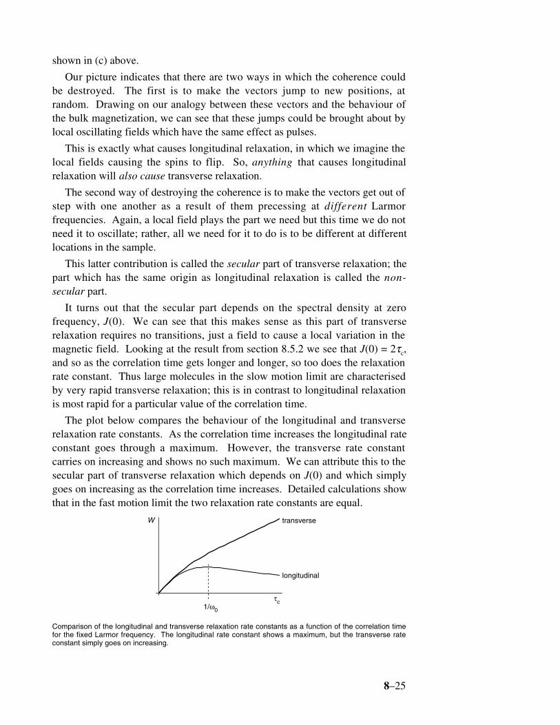
The plot below compares the behaviour of the longitudinal and transverserelaxation rate constants. As the correlation time increases the longitudinal rateconstant goes through a maximum. However, the transverse rate constantcarries on increasing and shows no such maximum. We can attribute this to thesecular part of transverse relaxation which depends on J(0) and which simplygoes on increasing as the correlation time increases. Detailed calculations showthat in the fast motion limit the two relaxation rate constants are equal.
τc1/ω0
W
longitudinal
transverse
Comparison of the longitudinal and transverse relaxation rate constants as a function of the correlation timefor the fixed Larmor frequency. The longitudinal rate constant shows a maximum, but the transverse rateconstant simply goes on increasing.