Embed Size (px)
Citation preview

Chapter 9Chapter 9
© 2006 Thomson Learning/South-Western
Profit Maximization and Supply
2
The Output Decision
Economic profits () are defined as = R(q) - TC(q) (9.1)
where R(q) is the amount of revenues received and TC(q) are the economic costs incurred, , both depending upon the level of output (q) produced.
The firm will choose the level of output that generates the largest level of profit.
3
The Output Decision
In Figure 9-1, (TC) is the total cost curve that is drawn consistent with the discussion in Chapter 8.
The total revenues curve is labeled (R). As drawn in the figure, profits reach their
maximum at the output level q*.

4
Costs (TC)
Revenues (R)
Profits
q1 q2q*
Costs,Revenue
(a)
(b)
Profits0
Outputper week0
FIGURE 9-1: Marginal Revenue Must Equal Marginal Cost for Profit Maximization
Outputper week
5
The Marginal Revenue/Marginal Cost Rule
At output levels below q* increasing output causes profits to increase, so profit maximizing firms would not stop short of q*.
Increasing output beyond q* reduces profits, so profit maximizing firms would not produce more than q*.

6
The Marginal Revenue/Marginal Cost Rule
At q* marginal cost equals marginal revenue, the extra revenue a firm receives when it sells one more unit of output.
In order to maximize profits, a firm should produce that output level for which the marginal revenue from selling one more unit of output is exactly equal to the marginal cost of producing that unit of output.
7
The Marginal Revenue/Marginal Cost Rule
At the profit maximizing level of output Marginal Revenue = Marginal Cost (9.2)
or MR = MC. (9.3)
Firms, starting at zero output, can expand output so long as marginal revenue exceeds marginal cost, but don’t go beyond the point where these two are equal.

8
Marginal Revenue
A price taker is a firm or individual whose decisions regarding buying or selling have no effect on the prevailing market price of a good or service.
For a price taking firm MR = P. (9.4)

9
Marginal Revenue for a Downward-Sloping Demand Curve
A firm that is not a price taker faces a downward sloping demand curve for its product.
These firms must reduce their selling price in order to sell more goods or services.
In this case marginal revenue is less than market price
MR < P. (9.5)

10
A Numerical Example
Assume the quantity demanded of CDs from a particular store per week (q) is related to the price (P) by
q = 10 - P. (9.6) Total revenue is (P·q) and marginal
revenue (MR) is the change in total revenue due to a change in quantity demanded.

11
A Numerical Example
This example demonstrates that MR < P as shown in Table 9-1.
Total revenue reaches a maximum at q = 5, P = 5.
For q > 5, total revenues decline causing marginal revenue to be negative.

12
TABLE 9-1: Total and Marginal Revenue for CDs (q = 10 - P)
Price (P)
Quantity (q)
Total Revenue (P·q)
Marginal Revenue (MR)
$10 0 $0 9 1 9 $ 9 8 2 16 7 7 3 21 5 6 4 24 3 5 5 25 1 4 6 24 -1 3 7 21 -3 2 8 16 -5 1 9 9 -7 0 10 0 -9

13
A Numerical Example
This hypothetical demand curve is shown in Figure 9-2.
When q = 3, P = $7 and total revenue equals $21 which is shown by the area of the rectangle P*Aq*0.
If the firm wants to sell four CDs it must reduce the price to $6.

14
Price(dollars)
Demand
AP* = $7
10
CDsper week1 2 3 4 10
q*0
FIGURE 9-2: Illustration of Marginal Revenue for the Demand Curve for CDs (q = 10 - P)
15
A Numerical Example
Total revenue is not $24 as illustrated by the area of the rectangle P**Bq**0.
The sale of one more CD increases revenue by the price at which it sells ($6).
But, to sell the fourth CD, it must reduce its selling price on the first three CDs from $7 to $6 which reduces revenue by $3, which is shown in the lightly shaded rectangle.

16
Price(dollars)
Demand
A
B
P* = $7
10
CDsper week1 2 3 4 10
q* q**0
FIGURE 9-2: Illustration of Marginal Revenue for the Demand Curve for CDs (q = 10 - P)
P* = $6

17
A Numerical Example
The net result of this price decrease is total revenue increases by only $3 ($6 - $3).
Thus, the marginal revenue of the fourth CD is $3.
The sale of the sixth CD, instead of five, results in an increase in revenue of the price ($4), but a decrease for the five other CDs (-$5) with a net effect (MR) = -$1.
18
Marginal Revenue and Price Elasticity
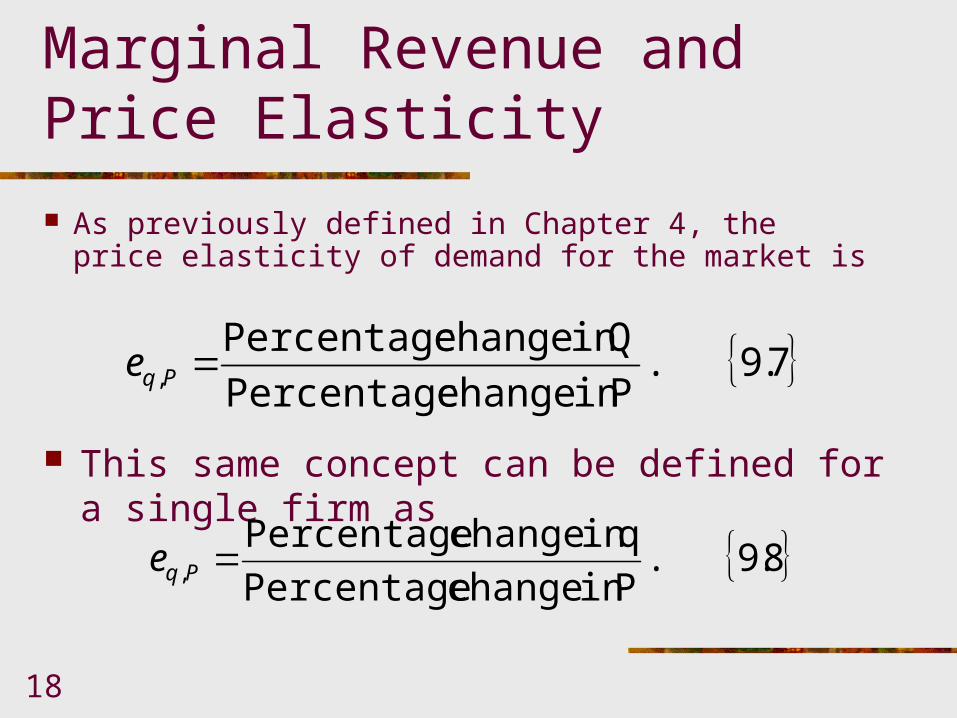
As previously defined in Chapter 4, the price elasticity of demand for the market is
This same concept can be defined for a single firm as
7.9., P in change Percentage
Q in change PercentagePqe
8.9., P in change Percentage
q in change PercentagePqe
19
Marginal Revenue and Price Elasticity
If demand facing the firm is inelastic
(0 eq,P > -1), a rise in the price will cause total revenues to rise.
If demand is elastic (eq,P < -1), a rise in price will result in smaller total revenues.
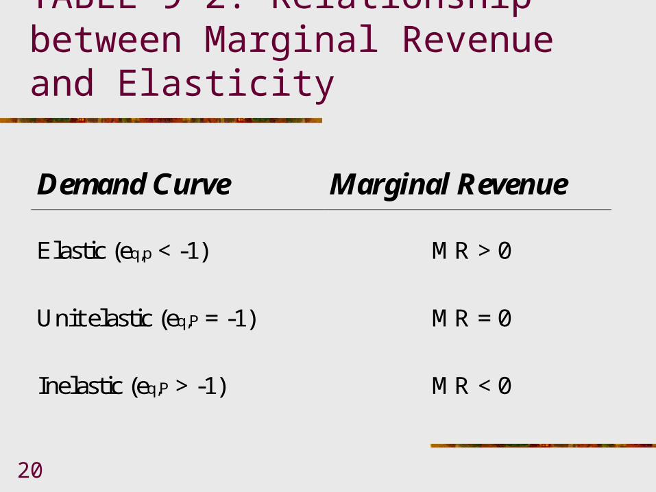
This relationship between the price elasticity and marginal revenue is summarized in Table 9-2.
20
TABLE 9-2: Relationship between Marginal Revenue and Elasticity
Demand Curve Marginal Revenue
Elastic (eq,p < -1) MR > 0
Unit elastic (eq,P = -1) MR = 0
Inelastic (eq,P > -1) MR < 0
21
Marginal Revenue and Price Elasticity
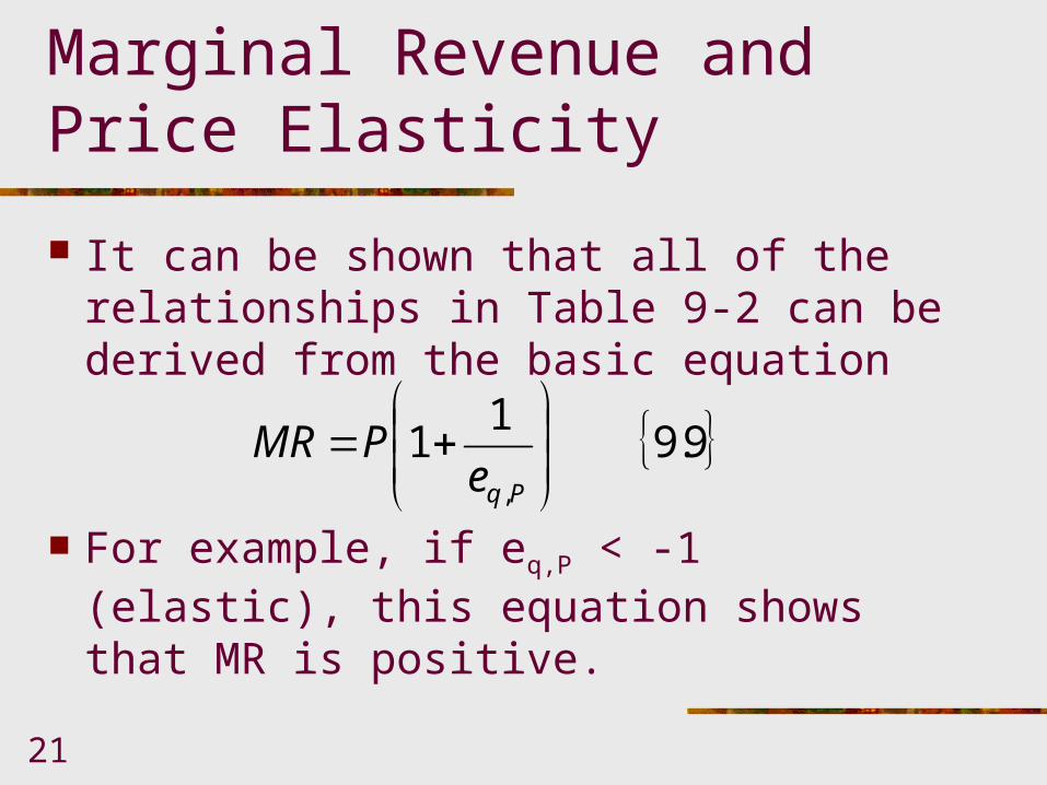
It can be shown that all of the relationships in Table 9-2 can be derived from the basic equation
For example, if eq,P < -1 (elastic), this equation shows that MR is positive.
9.91
1,
PqePMR
22
Marginal Revenue and Price Elasticity
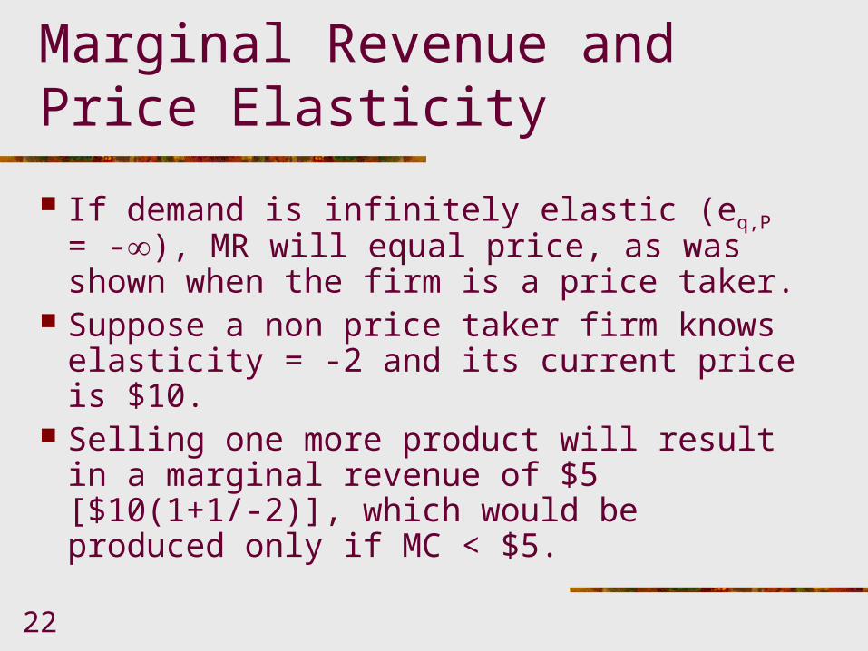
If demand is infinitely elastic (eq,P = -), MR will equal price, as was shown when the firm is a price taker.
Suppose a non price taker firm knows elasticity = -2 and its current price is $10.
Selling one more product will result in a marginal revenue of $5 [$10(1+1/-2)], which would be produced only if MC < $5.
23
Marginal Revenue Curve
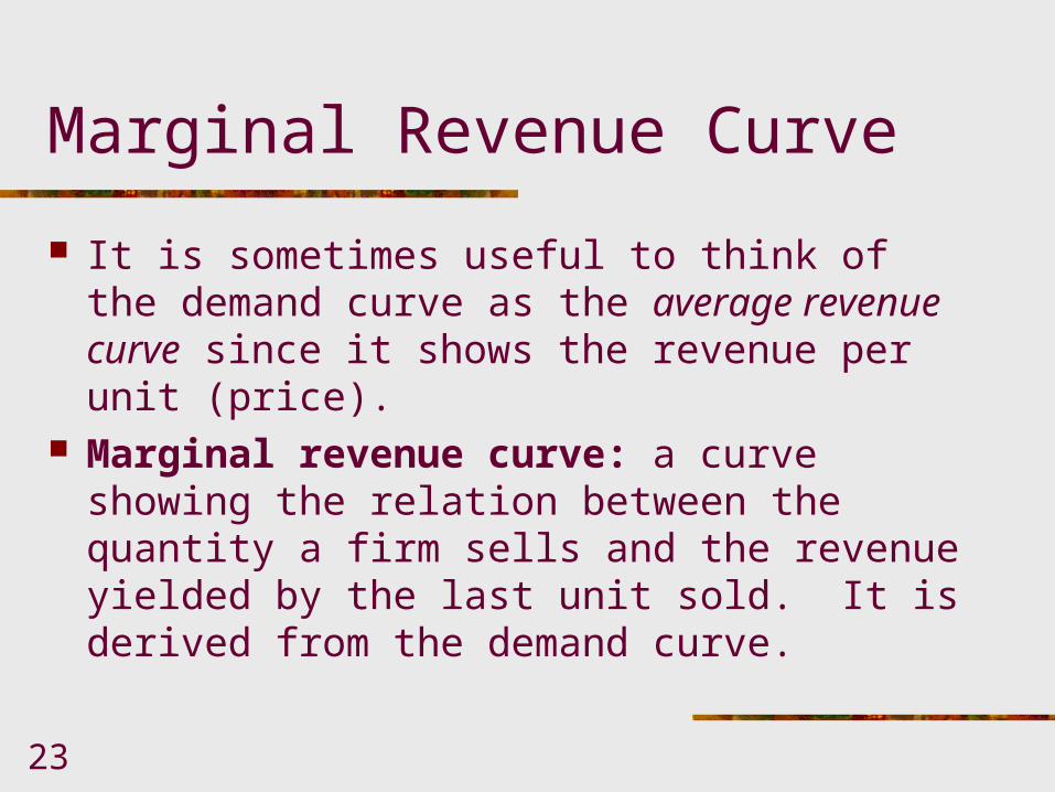
It is sometimes useful to think of the demand curve as the average revenue curve since it shows the revenue per unit (price).
Marginal revenue curve: a curve showing the relation between the quantity a firm sells and the revenue yielded by the last unit sold. It is derived from the demand curve.

24
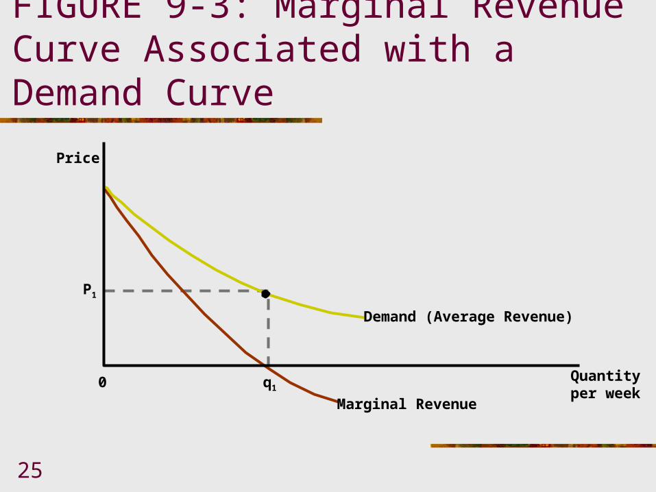
Marginal Revenue Curve
With a downward-sloping demand curve, the marginal revenue curve will lie below the demand curve since, at any level of output, marginal revenue is less than price.
A demand and marginal revenue curve are shown in Figure 9-3.
For output levels greater than q1, marginal revenue is negative.
25
Price
Demand (Average Revenue)
Marginal Revenue
P1
Quantityper week
q10
FIGURE 9-3: Marginal Revenue Curve Associated with a Demand Curve
26
Shifts in Demand and Marginal Revenue Curves
As previously discussed, changes in such factors as income, other prices, or preferences cause demand curves to shift.
Since marginal revenue curves are derived from demand curves, whenever the demand curve shifts, the marginal revenue curve also shifts.
27
Short-Run Profit Maximization
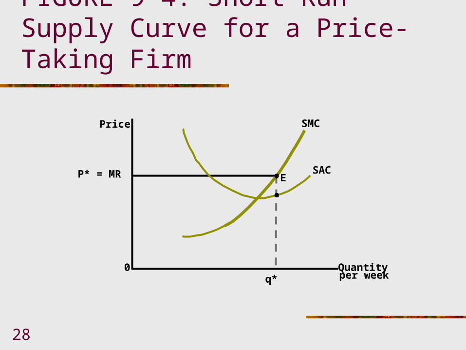
Since the firm has no effect on the price it receives for its product, the goal of maximizing profits dictates that it should produce the quantity for which marginal cost equals price.
At a given price, such as P* in Figure 9-4, the firm’s demand curve is a horizontal line through P*.
28
Price
P* = MR
0 Quantityper week
SAC
SMC
E
q*
FIGURE 9-4: Short-Run Supply Curve for a Price-Taking Firm
29
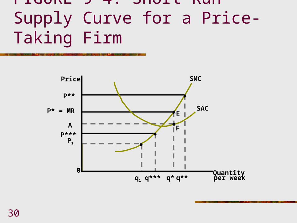
Short-Run Profit Maximization
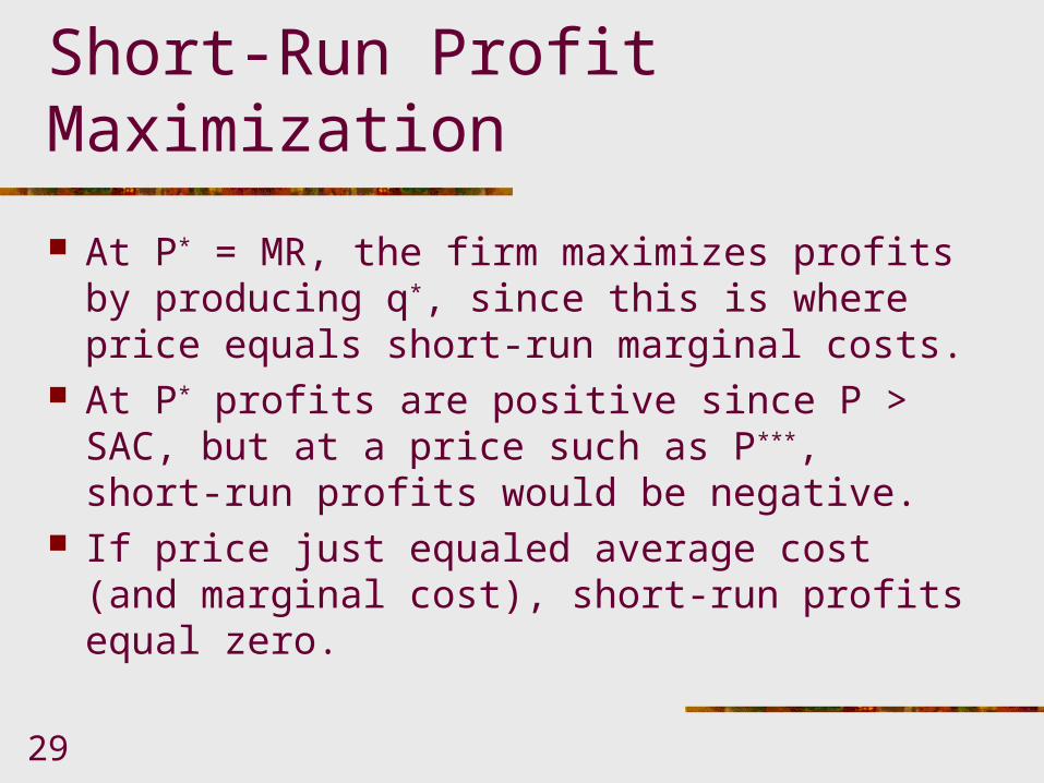
At P* = MR, the firm maximizes profits by producing q*, since this is where price equals short-run marginal costs.
At P* profits are positive since P > SAC, but at a price such as P***, short-run profits would be negative.
If price just equaled average cost (and marginal cost), short-run profits equal zero.
30
Price
P* = MR
P**
AP***
P1
0 Quantityper week
SAC
SMC
E
F
q1 q*** q* q**
FIGURE 9-4: Short-Run Supply Curve for a Price-Taking Firm

31
Short-Run Profit Maximization
If, at P* the firm produced less than q*, profits could be increased by producing more since MR > SMC below q*.
Alternatively, if the firm produced more than q* profits could be increased by producing less since MR < SMC beyond q*.
Thus, profits can only be maximized by producing q* when price is P*.
32
Short-Run Profit Maximization
Total profits are given by the area P*EFA which can be calculated by multiplying profits per unit (P* - A) times the firm’s chosen output level q*.
For this situation to truly be a maximum profit, the marginal cost curve must also be increasing (it would be a profit minimum if the marginal cost curve was decreasing).

33
The Firm’s Short-Run Supply Curve
The firm’s short-run supply curve is the relationship between price and quantity supplied by a firm in the short-run.
For a price-taking firm, this is the positively sloped portion of the short-run marginal cost curve.
For all possible prices, the marginal cost curve shows how much output the firm should supply.

34
The Shutdown Decision
The firm will opt for q > 0 providing
The price must exceed average variable cost.
16.9.
15.9
q
SVCP
SVCqP
q,by dividing or,

35
The Shutdown Decision
The shutdown price is the price below which the firm will choose to produce no output in the short-run. It is equal to minimum average variable costs.
In Figure 9-4, the shutdown price is P1. For all P P1 the firm will follow the P =
MC rule, so the supply curve will be the short-run marginal cost curve.
36
The Shutdown Decision
Notice, the firm will still produce if P < SAC, so long as it can cover its fixed costs.
However, if price is less than the shutdown price (P < P1 in Figure 9-4), the firm will have smaller losses if it shuts down.
This decision is illustrated by the colored segment 0P1 in Figure 9-4.

37
Price
P1
0Quantityper week
SMC
FIGURE 9-4: Short-Run Supply Curve for a Price-Taking Firm