Chapter 9

Exercise 9.10.1

Alice is violating the standard monotonicity assumption that she always prefers more

eggs over less eggs.

1

Chapter 9

Exercise 9.10.2

(a) 3;

(b) 2af ;

(c) 1f√

a+2a.

2

Chapter 9

Exercise 9.10.3

∇u (f, a) = (2af, a2), the equation of the tangent plane at (A, F )T is 3A2F =

a 2AF + fA2, where (a, f) denotes a point on the plane (notice that the tangent

plane is in fact a line).

3

Chapter 9

Exercise 9.10.4

We need to solve for points (a, f) satisfying λ (2af, a2) = (f 2, 2af), which gives us

the following equations: 2λa = f , λa = 2f . This gives the solution f = 0 and either

λ = 0 or a = 0. At these points, which are common to indifference curves of both

agents, the tangent planes to these indifference curves are also common. This means

that the indifference curves touch at these points.

4

Chapter 9

Exercise 9.10.5

π (w) = r (w)− c (w), so π′ (w) = 0 is the same as r′ (w) = c′ (w). Assuming revenue

to be concave and cost to be convex, this is the condition for the maximum of the

profit function. At the minimum of π (.) it will then be r′ (w) < c′ (w), and the

minimum will be achieved either at w = 0 or at w = wmax.

5

Chapter 9

Exercise 9.10.6

Adam’s indifference curve in the (f, p) space is (A − pf) f 2 = c where c is a constant.

To obtain his demand we have to maximize his utility as a function of f , at a given

price p. That is, 2Af − 3pf 2 = 0, yielding the demand curve f = 2A3p

.

6

Chapter 9

Exercise 9.10.7

Bob’s demand is found by max a2f given that pf + qa ≤ M . At the maximum, this

constraint has to hold with equality, thus we have to compute max a2

p(M − qa). This

gives us Bob’s demand for apples a = 2M3q

. Using the relation pf + qa = M we then

get his demand fot fig leaves f = M3p

. N copies of of Bob will demand N times as

much apples and fig leaves at given prices.

7

Chapter 9

Exercise 9.10.8

If Alice fixes prices p and q then her revenue is N(

pM3p

+ q 2M3q

)

= NM . Suppose her

unit cost of producing fig leaves is 0 and the cost of producing an apple is c > 0.

Then her profit if prices are p and q is π (p, q) = NM − cN 2M3q

. This implies that

she gets the highest profit when q is infinite, and the demand for apples is 0.

8

Chapter 9

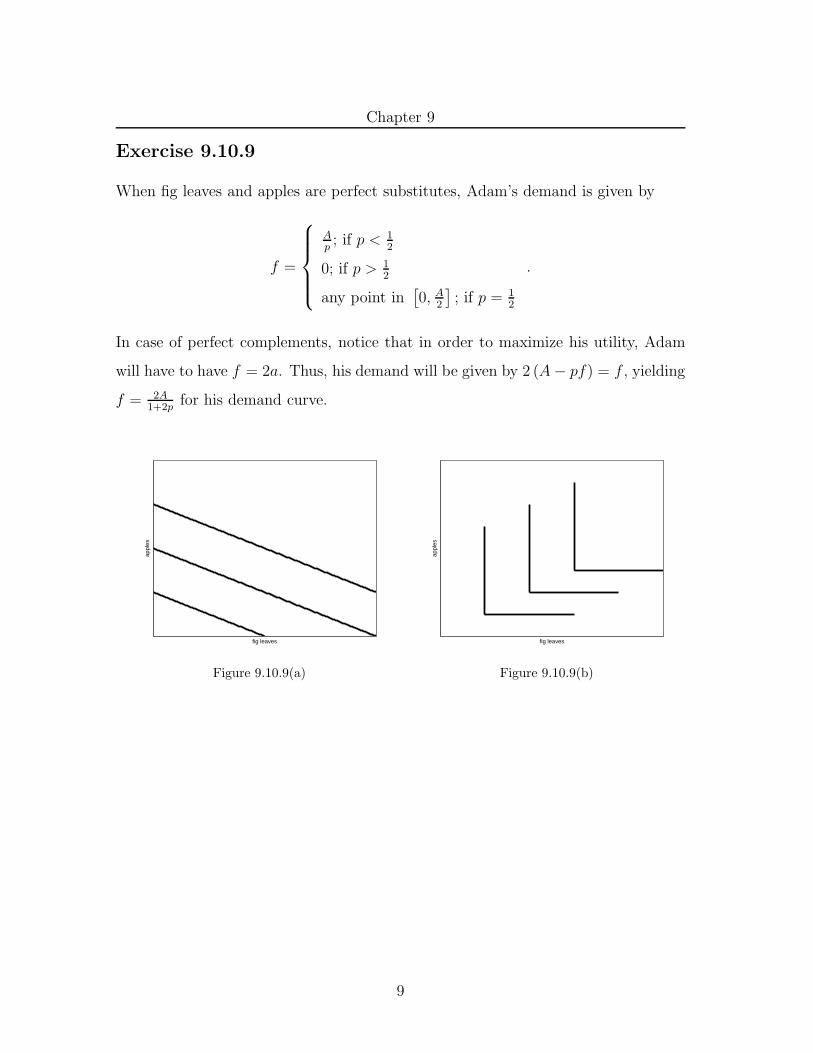
Exercise 9.10.9

When fig leaves and apples are perfect substitutes, Adam’s demand is given by

f =

Ap; if p < 1

2

0; if p > 12

any point in[

0, A2

]

; if p = 12

.

In case of perfect complements, notice that in order to maximize his utility, Adam

will have to have f = 2a. Thus, his demand will be given by 2 (A − pf) = f , yielding

f = 2A1+2p

for his demand curve.

fig leaves

appl

es

Figure 9.10.9(a)

fig leaves

appl

es

Figure 9.10.9(b)

9

Chapter 9

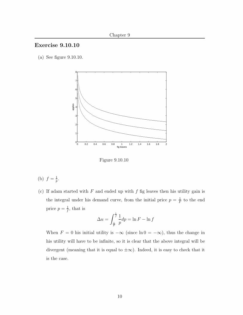
Exercise 9.10.10

(a) See figure 9.10.10.

0 0.2 0.4 0.6 0.8 1 1.2 1.4 1.6 1.8 20

1

2

3

4

5

6

7

8

fig leaves

appl

es

Figure 9.10.10

(b) f = 1p.

(c) If adam started with F and ended up with f fig leaves then his utility gain is

the integral under his demand curve, from the initial price p = 1F

to the end

price p = 1f, that is

∆u =

∫ 1

f

1

F

1

pdp = ln F − ln f

When F = 0 his initial utility is −∞ (since ln 0 = −∞), thus the change in

his utility will have to be infinite, so it is clear that the above integral will be

divergent (meaning that it is equal to ±∞). Indeed, it is easy to check that it

is the case.

10

Chapter 9

Exercise 9.10.11

To find the contract curve we first find the set of efficient trades by solving for

points where ∇u (f, a) = λ∇u (F − f, A − a). In case (a) this gives us two equations

(2af, f 2) = λ(

−2 (A − a) (F − f) ,− (F − f)2), so if we divide them, we obtain the

equality af

= (A−a)(F−f)

(notice that this is the equality of marginal rates of substitution).

We can rearrange this to get the set of all efficient outcomes: a = A f

F, f ∈ [0, F ].

Since the utilities of the agents are 0 at their initial endowment, this is also the

contract curve. At the Walrasian equilibrium we have that the price vector (p, 1) also

points into the same direction as the utility gradients of both agents, which means

that we get an additional equation (again by dividing to get rid of the multiplyer),

p

1= a

f. Along with the budget constraint (take for instance Adam’s), pf = A − a,

this gives us sufficiently many equations to compute the Walrasian equilibrium - we

can solve for p in terms of a and f , then plug in the expression for a, and finally nail

down the solution for f with the remaining equation. The Walrasian equilibrium

is f = F2, a = A

2, and p = A

F. For case (b) we can proceed in the same way, to

obtain the contract curve a = f(A+2)−F+A

F+2, where we now have to be careful with the

interval of possible values for f , which are determined from the condition that each

agent get at least as much utility as his initial endowment gives him.

11

Chapter 9

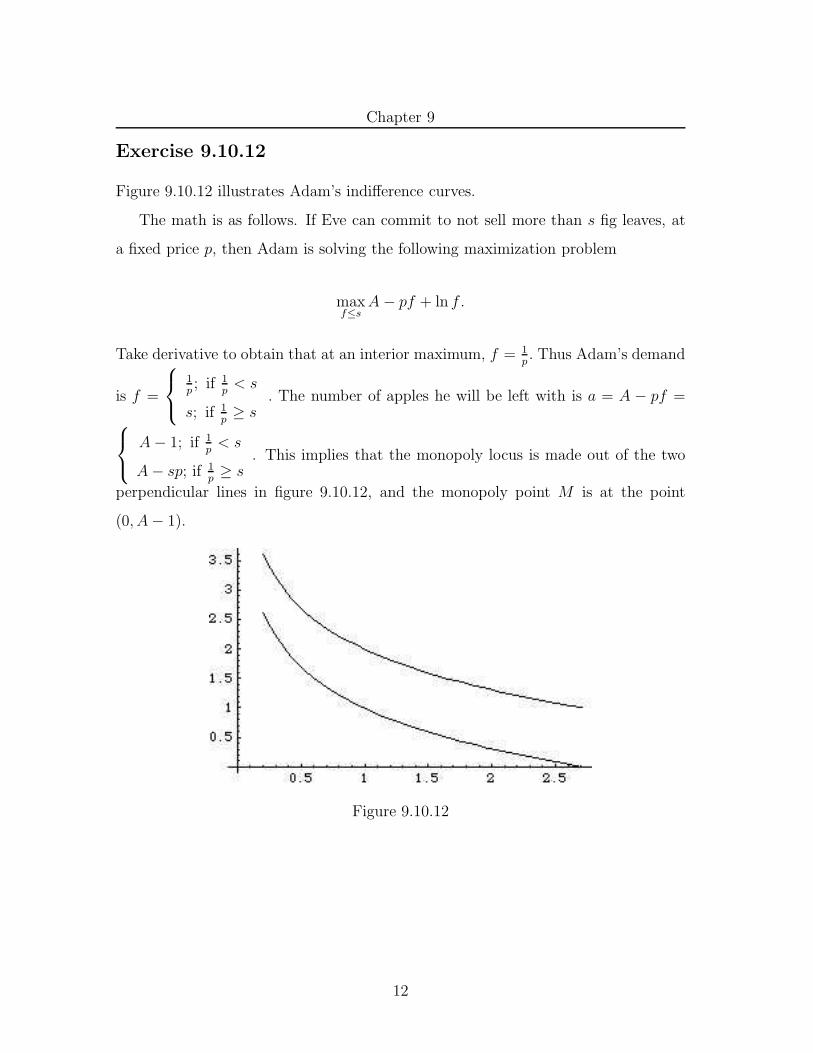
Exercise 9.10.12

Figure 9.10.12 illustrates Adam’s indifference curves.

The math is as follows. If Eve can commit to not sell more than s fig leaves, at

a fixed price p, then Adam is solving the following maximization problem

maxf≤s

A − pf + ln f .

Take derivative to obtain that at an interior maximum, f = 1p. Thus Adam’s demand

is f =

1p; if 1

p< s

s; if 1p≥ s

. The number of apples he will be left with is a = A − pf =

A − 1; if 1p

< s

A − sp; if 1p≥ s

. This implies that the monopoly locus is made out of the two

perpendicular lines in figure 9.10.12, and the monopoly point M is at the point

(0, A − 1).

Figure 9.10.12

12

Chapter 9

Exercise 9.10.13

u (f, a) = min {f, a}.

(a) See the solution to 9.10.9.

(b) The demand is obtained as the intersection of the budget line a+pf = A+pF .

and the line on which the indifference curves have the kink, a = f

2. Thus, the

demand is f = A+pF

p+ 1

2

.

(c) If we integrate the area under the demand curve from the price at the initial

endowment, p = ∞, to some price p0 we obtain

∫ ∞

p0

(

A + pF

p + 12

)

dp =

∫ ∞

p0

(

F +A − F

2

p + 12

)

dp =

(

Fp −(

A − F

2

)

ln

(

p +1

2

))∞

p0

= ∞

Obviously, the change in Adam’s utility is not infinite - notice that his utility

isn’t quasi-linear. For the case where u (f, a) = f +2a the analysis is analogous

to the analysis of exercise 9.10.10 since his utility function is then again quasi-

linear, except that there are no problems when F = 0.

13

Chapter 9

Exercise 9.10.14

First compute Adam’s demand: maxf (A − p (f − F ))2f , which gives the condition

(A − p (f − F )) (A − p (3f − F )) = 0. One root of this equation is a local minimum

of Adam’s utility, and the other one gives the demand f = 13

(

Ap

+ F)

. A perfectly

discriminating monopolist charges the lowest price p = 1, which is obtained when

f = A+F3

. So the area under the demand function is

A+F3∫

F

3f − F

Adf =

1

6A

(

A2 − 4F 2)

.

On the other hand, the monopolist trade point is the intersection of Adam’s indiffer-

ence curve a2f = A2F with the contract curve 2f = a (it is immediate to compute

that this is the contract curve). That is, f = 3

√

A2F4

and a =3√

2A2F , and since

Alice’s profit is π = A − a − (f − F ) the above integral is clearly not equal to π.

14

Chapter 9

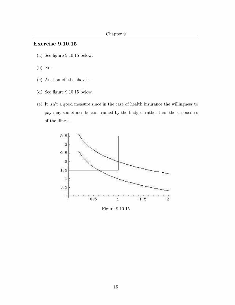
Exercise 9.10.15

(a) See figure 9.10.15 below.

(b) No.

(c) Auction off the shovels.

(d) See figure 9.10.15 below.

(e) It isn’t a good measure since in the case of health insurance the willingness to

pay may sometimes be constrained by the budget, rather than the seriousness

of the illness.

Figure 9.10.15

15

Chapter 9

Exercise 9.10.16

Since the pumping stations know that the next day the price will be higher, they

want to keep the supply down in order to hike up the price already on the given

day. Another way to put this is that since the price will go up the next day, their

opportunity cost of sales on the given day is increased, so the supply curve shifts

upward.

16

Chapter 9

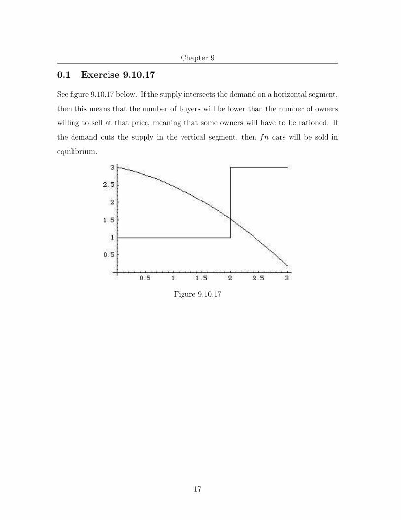
0.1 Exercise 9.10.17

See figure 9.10.17 below. If the supply intersects the demand on a horizontal segment,

then this means that the number of buyers will be lower than the number of owners

willing to sell at that price, meaning that some owners will have to be rationed. If

the demand cuts the supply in the vertical segment, then fn cars will be sold in

equilibrium.

Figure 9.10.17

17

Chapter 9

Exercise 9.10.18

(a) This is very simple and follows directly from the definition of expectation.

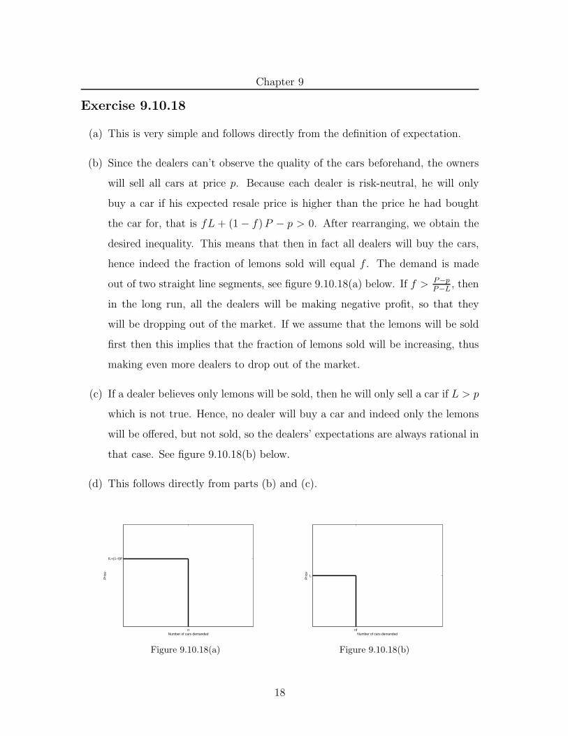
(b) Since the dealers can’t observe the quality of the cars beforehand, the owners

will sell all cars at price p. Because each dealer is risk-neutral, he will only

buy a car if his expected resale price is higher than the price he had bought

the car for, that is fL + (1 − f)P − p > 0. After rearranging, we obtain the

desired inequality. This means that then in fact all dealers will buy the cars,

hence indeed the fraction of lemons sold will equal f . The demand is made

out of two straight line segments, see figure 9.10.18(a) below. If f > P−p

P−L, then

in the long run, all the dealers will be making negative profit, so that they

will be dropping out of the market. If we assume that the lemons will be sold

first then this implies that the fraction of lemons sold will be increasing, thus

making even more dealers to drop out of the market.

(c) If a dealer believes only lemons will be sold, then he will only sell a car if L > p

which is not true. Hence, no dealer will buy a car and indeed only the lemons

will be offered, but not sold, so the dealers’ expectations are always rational in

that case. See figure 9.10.18(b) below.

(d) This follows directly from parts (b) and (c).

n

fL+(1−f)P

Number of cars demanded

Pric

e

Figure 9.10.18(a)

nf

L

Number of cars demanded

Pric

e

Figure 9.10.18(b)

18

Chapter 9

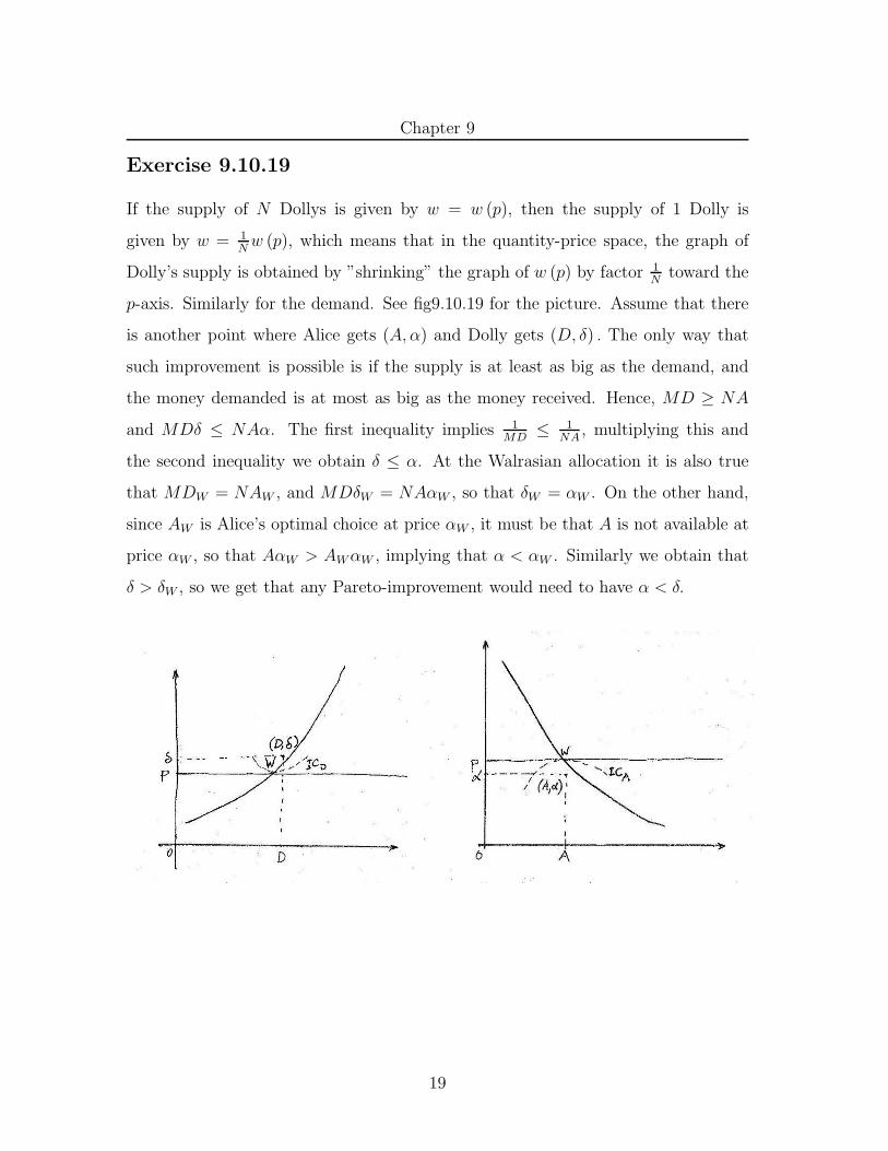
Exercise 9.10.19

If the supply of N Dollys is given by w = w (p), then the supply of 1 Dolly is

given by w = 1N

w (p), which means that in the quantity-price space, the graph of

Dolly’s supply is obtained by ”shrinking” the graph of w (p) by factor 1N

toward the

p-axis. Similarly for the demand. See fig9.10.19 for the picture. Assume that there

is another point where Alice gets (A, α) and Dolly gets (D, δ) . The only way that

such improvement is possible is if the supply is at least as big as the demand, and

the money demanded is at most as big as the money received. Hence, MD ≥ NA

and MDδ ≤ NAα. The first inequality implies 1MD

≤ 1NA

, multiplying this and

the second inequality we obtain δ ≤ α. At the Walrasian allocation it is also true

that MDW = NAW , and MDδW = NAαW , so that δW = αW . On the other hand,

since AW is Alice’s optimal choice at price αW , it must be that A is not available at

price αW , so that AαW > AWαW , implying that α < αW . Similarly we obtain that

δ > δW , so we get that any Pareto-improvement would need to have α < δ.

19

Chapter 9

Exercise 9.10.20

Let (AW , αW ) and (DW , δW ) be the Walrasian allocation, and let (A0, α0) and (D0, δ0)

be the initial allocation of wool and money. Let p be the Walrasian price of wool (price

of money is normalized at 1), and suppose there existed Pareto-improving bundles

(A, α) and (D, δ), and suppose that (A, α) is a strict improvement for Alice. Then it

must be that at price p, (A, α) was unaffordable to Alice, so that Ap+α > AWp+αW .

Similarly, for Dolly, the bundle (D, δ) must have been weakly unaffordable, Dp+δ ≥DWp + δW . This implies that (D + A)p + α + δ > (DW + AW )p + αW + δW . By

assumption, (A, α) and (D, δ) are feasible, so that A + D = A0 + D0 and α + δ =

α0 + δ0. Since Walrasian allocation is feasible, we also have DW + AW = A0 + D0

and αW + δW = α0 + δ0, hence, (A + D)p + α + δ = (DW + AW )p + αW + δW , which

is a contradiction.

20

Chapter 9

Exercise 9.10.21

The following reserve prices will work. On the supply side: pSi = i, and on the

demand side pDj = j for i = 1, ..., 10 and j = 1, ..., 10. Then any price p ∈ [5, 6] will

be a Walrasian equilibrium price because at any such price there will be precisely 5

sellers willing to sell and 5 buyers willing to buy. Suppose the buyers tell the truth

about their reserve prices. Then the Walrasian price will be set at p = 6. So all the

buyers with reserve prices strictly more than 6 will be happier with telling the truth

and trading than lieing and not trading. The buyer with reserve price exactly equal

to 6 is indifferent between telling the truth or not, since his net gain is 0 in any case.

So all the buyers are playing a best response. Clearly, the sellers are playing a best

reply strategy since they do not really move anyway. So this is a Nash equilibrium.

21

Chapter 9

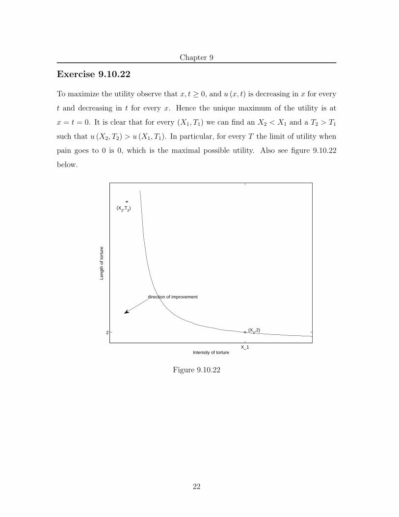
Exercise 9.10.22

To maximize the utility observe that x, t ≥ 0, and u (x, t) is decreasing in x for every

t and decreasing in t for every x. Hence the unique maximum of the utility is at

x = t = 0. It is clear that for every (X1, T1) we can find an X2 < X1 and a T2 > T1

such that u (X2, T2) > u (X1, T1). In particular, for every T the limit of utility when

pain goes to 0 is 0, which is the maximal possible utility. Also see figure 9.10.22

below.

X_1

2

Intensity of torture

Leng

th o

f tor

ture

(X1,2)

(X2,T

2)

direction of improvement

Figure 9.10.22

22