Embed Size (px)
Citation preview

Chapter 9 FINITE ELEMENT ANALYSIS OF CHALK BEHAVIOR
MATERIAL NONLINEARITY AND THE INITIAL STRESS METHOD
The displacement finite element formulation is described in detail in several references
(Zienkiewicz and Taylor, 2000; Hughes, 2000). The basics of the formulation are omitted here.
A description of the initial stress method (Zienkiewicz et al., 1969) to account for material
nonlinearity is given in the following paragraphs.
Using the displacement finite element method, a vector of incremental nodal
displacements ∆u is related to the vector of applied incremental nodal forces ∆F by the global
stiffness matrix K for the structure being analyzed:
uKF ∆=∆ (9.1)
For finite element analyses, the incremental nodal forces are generally known while the
incremental nodal displacements are sought.
The global stiffness matrix is calculated using some stiffness tensor D, usually the elastic
De or tangent elastoplastic constitutive stiffness tensor Dep:
(9.2) ∫=V
T dVDBBK
In equation (9.2), V is the element volume and B is the strain-displacement tensor, representing
the derivatives of the element shape functions N. The global stiffness matrix is the sum of all
element stiffnesses in the finite element mesh.
The load-displacement curve is nonlinear for materials which exhibit material
nonlinearity, such as geomaterials (Figure 9.1).Therefore, the displacements calculated using
equation (9.1) generally correspond to stresses which are not in agreement with the constitutive
behavior the material. The nodal displacements must be corrected such that the stresses
correspond to the constitutive behavior of the material, and the applied external forces are in
equilibrium with the stresses within each element. The initial stress method described here is one
procedure used to accomplish this.
For the initial stress method, the strain increment vector ∆ε at each Gauss point may be
calculated using the strain-displacement matrix:
uBε ∆=∆ (9.3)
291

A trial stress σtr may be calculated using the constitutive stiffness tensor D which was used to
form the element stiffness matrix for the element of interest:
(9.4) εDσσσσ ∆+=∆+= 00 etr
The stress increment ∆σe in equation (9.4) represents the elastic stress increment, which reflects
the fact that the elastic stiffness tensor is usually the constitutive stiffness tensor D which is
usually used to form the global stiffness matrix.
As stated above, the trial stress σtr generally is not in agreement with the applied strain
increment and the constitutive behavior for geomaterials. A converged final stress σf must be
calculated using the constitutive equations for the material and an appropriate integration
algorithm. The stress correction ∆σ between the trial and final stresses is converted into a nodal
elemental force vector ∆Fel:
(9.5) ftr σσσ −=∆
(9.6) ∫ ∆=∆V
Tel dVσBF
The nodal force vectors for all elements are summed into a global correction force vector ∆F and
then applied to the structure using equation (9.1) to bring the structure into global force
equilibrium (Figure 9.1). If the yield function f < 0 for all Gauss points in the structure, any
required stress correction is due to time-dependent behavior and only a single corrective iteration
is needed to attain global force equilibrium; if the yield function f = 0 for any Gauss points in the
structure, multiple corrective iterations using the initial stress method are usually required to
achieve force equilibrium (Figure 9.1). The initial stress method illustrated in Figure 9.1 uses the
Newton-Raphson method to achieve global equilibrium, in which the tangent global stiffness
matrix is formed at each iteration to calculate the incremental displacements.
The finite element code used for the simulations was implemented on a MATLAB
platform. The code uses 8-noded three-dimensional quadratic elements with a linear
displacement function in each dimension. The shape functions for each element are evaluated at
eight Gauss points (two in each dimension). Global equilibrium is attained using the Modified
Newton-Raphson procedure, in which the initial global stiffness matrix is used for all global
iterations within a given loading step.
292

FINITE ELEMENT AMALYSIS OF PORE FLUID EFFECTS ON CHALK BEHAVIOR
The constitutive equations developed in Chapters 5, 6, and 8 to describe the behavior of North
Sea chalks and other soft rocks apply at a given point in a continuum. To use the constitutive
equations in finite element analysis, the strains and stresses are calculated at selected points (i.e.,
Gauss points) in each finite element. The displacements for each node of the finite element mesh
are calculated assuming that the same material properties apply at all points in a given finite
element. Since the water saturation is generally not uniform throughout the element, the average
properties which correspond to the average water saturation in an element are used to calculate
the average values for the material properties which apply to that element. This procedure is
based on a concept called “equivalent uniform water saturation.”
Use of the equivalent uniform water saturation is shown conceptually in Figure 9.2. The
weighted relative strength distribution in the element is first calculated as a function of the water
saturation distribution in the element. This relative strength corresponds to an equivalent uniform
relative strength and equivalent uniform water saturation everywhere in the element. For all
model parameters, it is assumed for calculation purposes that the equivalent uniform water
saturation and equivalent uniform relative strength are present everywhere in the element. An
example is given in the following paragraphs.
For a model parameter which varies as a function of water saturation, the appropriate
value of the parameter may be calculated if the water saturation is known. As described in
Chapter 8, it is assumed that the value of parameter x varies as a function of water saturation Sw
as follows:
( )( )bwSxxxx −−+= 1minmaxmin (9.7)
where xmax and xmin are the maximum and minimum values of parameter x, corresponding to
fully oil-saturated and fully water saturated conditions, respectively, and b is a fitting parameter.
If xmax = 2, xmin = 1, and b = 20, then x = 1.12 for a water saturation Sw = 0.1. This value of
parameter x is obtained for any saturation conditions in which one-tenth of the pore space in a
given finite element is occupied by water; this applies if one-tenth of the pore space is fully
water-saturated and nine-tenths is fully oil-saturated, if all the pores are saturated with a fluid
that contains 10% water plus 90% oil, or for any intermediate saturation condition.
293

FINITE ELEMENT SIMULATIONS
Three finite element simulations have been performed to demonstrate the ability of the
constitutive model and finite element code to simulate the behavior of chalk at different scales. A
description of the finite element simulations follows:
1) Laboratory scale simulations: These simulations examine the effects of one-dimensional
waterflooding and uniaxial compaction of a chalk sample in a laboratory apparatus due to
water injection and movement of the waterfront through an initially oil-saturated sample.
It is assumed that the waterfront moves through the sample at a constant rate in a piston-
like manner. The water saturation is assumed to be its maximum value in the volume of
sample that the waterfront has passed, and to be its minimum value in the volume of
sample that the waterfront has not reached. Several simulations are performed to illustrate
the influence of stress states, waterflooding rates, and sample discretization on the
simulated mechanical behavior of chalk. The cylindrical sample has dimensions of 2
inches in length and 2 inches in diameter (Figure 9.3). The first two simulations replicate
“fast” waterflooding in which the entire waterflooding procedure takes 2 hours; these
loading conditions are similar to those of Homand and Shao (2000). For all simulations,
all elements have an initial porosity of 0.42; the equivalent void ratio is 0.72. The values
used for the material properties are shown in Table 9.1. One simulation is performed
under hydrostatic stress conditions (σa = σr = 18 MPa), while the other is performed
under near-K0 conditions (σa = 22.7 MPa, σr = 14 MPa). For both simulations, a quarter-
section of the sample is analyzed with the finite element mesh discretized into 20
elements in the axial direction. 40 loading steps are applied for both simulations in the
first set. The second two simulations replicate a “slow” waterflooding in which a 40-hour
waterflood is performed between two 180-hour creep stages; these loading conditions are
similar to those for the waterflooding tests detailed in Chapter 8. Both simulations are
performed under near- K0 conditions (σa = 22.7 MPa, σr = 14 MPa). A quarter-section of
the sample is analyzed with different discretizations; for one simulation, the 20-element
discretization in the axial direction is used, while a 1-element structure is used in the
second simulation. For the 20-element structure, it is assumed that the water saturation
increases at a constant rate in each successive element as the simulated waterfront passes;
294

when one element becomes fully water-saturated, the next element starts to become
waterflooded. For the 1-element structure, it is assumed that the water saturation
increases at a constant rate, uniformly throughout the single element. 200 loading steps
are applied for both simulations in this second set. A comparison between the second two
simulations will demonstrate the use of the averaging procedure and the “equivalent
uniform water saturation” concept as described in the previous section.
2) Borehole scale simulations: These simulations examine the effects of waterflooding in
the originally oil-saturated near-borehole region of an injection well. Again, it is assumed
that the waterfront moves through the chalk at a constant rate in a piston-like manner.
Three separate simulations are performed to investigate the relative effects of water
weakening (or change in material behavior) and pore pressure increase which occur due
to water injection. The first simulation assumes only water weakening occurs; the second
simulation assumes only pore pressure increase occurs; and the third simulation assumes
both processes occur simultaneously. For all simulations, a quarter section of the near-
borehole region is analyzed (Figure 9.4). The borehole has a diameter of 0.8 m, and the
full section is a square with 80 m-long sides. The finite element mesh is discretized to
include 78 elements, with only one element in the z-direction. Deformation proceeds
under plane strain conditions. The initial stress conditions are slightly overconsolidated
and close to K0 conditions. The initial vertical effective stress for all elements in the mesh
is 30 MPa, while initial horizontal effective stress for all elements is 16 MPa. The initial
porosity for all elements is 0.35; the equivalent void ratio is 0.54. The values used for the
material properties are shown in Table 9.2. In each applicable case, water weakening
and/or pore pressure increase extends to a distance of 11 m from the center of the
borehole. The water saturation increases in the elements through which the waterfront
passes. In water-weakened regions, full water saturation is assumed. The pore pressure
increase dissipates with radial distance from the edge of the borehole. The maximum
increase in pore pressure is 10 MPa, adjacent to the borehole; the pore pressure increases
by 1 MPa at a radial distance of 11 m from the center of the borehole.
3) Field scale simulation: These simulations examine the effects of pore pressure drawdown
and oil production in the Ekofisk field. Two different simulations are performed to
examine the effects of water-weakening on reservoir compaction and subsidence. It is
295

assumed that the field chalk is initially oil-saturated, and that the initial fluid pressure in
the reservoir is equal everywhere. In both simulations, effective stresses increase
everywhere in the reservoir due to pore pressure drawdown. One simulation assumes no
weakening occurs; the other assumes that oil saturation is decreased by 1 percent
everywhere in the reservoir to account for historic oil production volume for the first 10
years of operations. In both cases, the field fluid pressure is decreased by 25 MPa in the
Ekofisk and Tor Formations (but not in the tight zone), which is equal to the maximum
historic drawdown. For all simulations, a quarter section of the near-borehole region is
analyzed (Figure 9.5). The full section is a parallelpiped with dimensions of 13 km x 10
km in plan view, and 3.6 km deep. The finite element mesh is discretized to include 315
elements. Deformation proceeds assuming that reservoir pressure (i.e., horizontal
stresses) are unchanged at the periphery of the mesh. The initial stress conditions are
slightly overconsolidated and close to K0 conditions. In the overburden and underburden
(layers 1-5 and 9), the initial vertical total stress gradient is 21 MPa/km. The fluid
pressure increases nonlinearly such that the initial fluid pressure in the reservoir is 49
MPa. The lateral earth pressure coefficients in the overburden and underburden, and
reservoir, are 0.8 and 0.3, respectively. All values are close to those recommended by
Nagel (1998). The initial porosity for all elements is 0.35; the equivalent void ratio is
0.54. The overburden and underburden are assumed to be transversely isotropic and
linear elastic with a greater stiffness in the x-y plane than in the vertical direction. The
reservoir is assumed to be isotropic and to follow the chalk model formulated in this
dissertation. The material stiffness in the reservoir assumed to equal half of the value
obtained from the correlations, and the plastic compressibility is doubled; these changes
are meant to account for reduced stiffness due to the presence of fractures. Similarly, the
elastic moduli chosen are equal to one-half those recommended by Nagel (1998). The
values used for the material properties are shown in Table 9.3.
RESULTS AND DISCUSSION
Laboratory-Scale Simulations
Results of the laboratory-scale simulations are presented in Figures 9.6 to 9.14 and are discussed
below. The strain-time results show the evolution of average strain over small intervals within
296

the sample, and are presented as if each element was instrumented with an individual strain
gauge. Also shown are the average axial strain over the entire length of the sample, which
represents the displacement of the piston in a triaxial cell. The axial intervals for which results
are presented are shown in Figure 9.6. Results for “fast” waterflooding simulations under
hydrostatic conditions and near-K0 conditions, respectively, are shown in Figures 9.7 and 9.8.
Figure 9.7 shows the evolution of axial and radial strain with time in four elements (elements 3,
8, 13, and 18) within the FE mesh for near-K0 conditions, while the equivalent figures for
hydrostatic stress conditions are shown in Figure 9.8. Figures 9.9 and 9.10 show the distribution
of pore space in the sample as loading progresses.
The results in Figures 9.7 and 9.8 agree qualitatively with the results of Schroeder et al.
(1998) and Homand and Shao (2000). The results indicate that (1) axial strain occurs in discrete
“jumps” as the waterflood passes and pore fluid composition changes; (2) the response of lateral
strain gauges occurs over longer time periods than that of the axial strain gauges; (3) radial
strains are of much greater magnitude, and axial strains are of lesser magnitude, under
hydrostatic stress conditions than under near-K0 stress conditions; (4) average axial strain
progresses at a nearly-constant rate during “fast” waterflooding events.
The results of Figures 9.9 and 9.10 indicate that at any given time, the distribution of
voids throughout the sample is bimodal. In oil-saturated regions of the sample, the void ratio is
very close to its original value, while in water-saturated regions, the void ratio is significantly
less. In each region, the void ratio is nearly uniform. These results indicate that pore collapse in
the chalk occurs immediately upon passage of the waterfront. The transition zone between the
more-porous (i.e., oil-saturated) region and less-porous (i.e., water-saturated) region moves in
the direction water flow as time passes. Evolution of void ratio in single-phase saturated regions
as time passes is attributed to creep.
For the creep and “slow” waterflooding test simulations, Figure 9.11 shows the evolution
of axial and radial strain, and void ratio, with time for the structure discretized into 20 elements.
Figure 9.12 shows the evolution of average axial and radial strain in the 1-element structure. It is
seen in Figure 9.11 that strain occurs uniformly throughout the sample during the initial creep
stage. However, strain becomes nonuniform during the waterflooding stage as described for the
fast waterflooding simulations, and remains nonuniform during the final creep stage. The
nonuniform strain signature is absent from the results for the 1-element structure shown in Figure
297
9.12, since only one element is present in the structure. The distribution of voids in the
discretized sample is shown in Figure 9.13. The distribution is uniform during the initial creep
stage; as for the “fast” waterflooding simulations, the void ratio distribution is nonuniform
during the waterflooding stage. However, the bimodal distribution of voids throughout the
sample is much less pronounced for the slow waterflooding simulations. A greater range of void
ratios is observed at any given time in Figure 9.13 than in either of Figures 9.9 or 9.10. These
effects may be attributed to time-dependent strains which occur at different rates at different
regions in the waterflooded region. Although the greatest reduction in void space is due to the
effects of waterflooding, post-waterflooding creep contributes to nonuniform distribution of void
space in the fully water-saturated region. At any given time, the greatest accumulated strain and
least void space are present in a region which was waterflooded earliest.
Figure 9.14 compares the average axial strain and radial strain signatures for the
simulations of the slow waterflooding test using the 20-element discretized FE mesh and using a
single element. The average strain histories are nearly identical at all times. It is concluded that
the algorithm using the “equivalent uniform water saturation” concept is able to represent the
same large-scale behavior for finite elements which are nonuniformly saturated with multiphase
fluids as for an assemblage of many finite elements with the same saturation conditions. The
algorithm gives good results even though the local behavior is quite different for chalk saturated
with different pore fluids.
Borehole-Scale Simulations
Results of the borehole-scale simulations are presented in Figures 9.15 to 9.20 and are discussed
below. The stress distributions at the end of the simulations are shown in Figures 9.15 to 9.17 for
the case in which waterflooding causes material weakening only, for the case in which
waterflooding causes pore pressure increase only, and for the case in which waterflooding causes
both material weakening and pore pressure increase, respectively. It may be seen in Figures 9.15
to 9.17 that radial and vertical stresses are all reduced in the waterflooded region, while the
stresses are not changed from their initial values in the oil-saturated region far from the borehole.
For the case in which only material weakening occurs, the tangential stresses increase adjacent to
the borehole, while the tangential stresses are reduced in the waterflooded region for the other
two cases. The stress state is that of hydrostatic compression (σ1 > σ2 = σ3) in the region far from
298

the borehole, while the stress state approaches that of hydrostatic extension (σ1 = σ2 > σ3) in the
near-borehole region, especially for the two cases which include pore pressure increase.
It is apparent from the results shown in Figures 9.15 to 9.17 that the stress distribution in
the waterflooded region is quite different for the three cases simulated. The distribution of each
stress component at the end of the simulation is shown as a function of the three waterflooding
cases considered in Figures 9.18 to 9.20. It is seen in Figure 9.18 that the distribution of radial
stress is very similar for the two cases which include a pore pressure increase, while the radial
stress is quite different for the case which includes material weakening only. In Figure 9.19, it
appears that the tangential stress distribution is slightly different for all three cases. Figure 9.20
shows that the distribution of vertical stress is very similar for the two cases which include
material weakening, while the vertical stress distribution is quite different for the case which
includes pore pressure increase only. For the case in which waterflooding causes material
weakening and pore pressure increase, all three stress components are reduced to their least
values for the three cases considered. It may be concluded that the pore pressure increase caused
by waterflooding most strongly influences the radial stress, while the material weakening caused
by waterflooding has its greatest influence on the vertical stress. While the radial and vertical
stresses are directly influenced by the effects of waterflooding, the tangential stress is less
directly dependent on these effects and more dependent on the relative magnitudes of the radial
and vertical stresses.
Field-Scale Simulations
Results for the two field-scale simulations are shown in Figures 9.21 to 9.24. Figures 9.21 show
the maximum compaction and subsidence profiles in the North-South and East-West direction
for the case in which no water-weakening occurs. Figure 9.22 shows the compaction and
subsidence histories at the center of the reservoir for the same simulation. Figures 9.23 and 9.24
are the corresponding figures for the water-weakening case.
It may be seen that for both cases, compaction is greatest at the reservoir center and is
generally restricted to the reservoir area, while the area of subsidence extends beyond the
reservoir limits. The compaction-to-subsidence (C/S) ratio for both cases is very close to the
measured value of 1.2. In both cases, the C/S ratio is approximately constant throughout the
depressurization phase. It is seen that the compaction and subsidence rates increase greatly when
299

depressurization exceeds 15 MPa, indicating that inelastic deformation becomes dominant as
effective stress increases.
The compaction and subsidence values increase substantially for the case in which water-
weakening occurs. Even a 1 percent change in water saturation has great effects on subsidence. It
may then be expected that continued operation of the field will lead to continued subsidence due
to water-weakening.
REFERENCES Gutierrez, M.S., Pokharel, G., and Hickman, R.J. (2004). JCRCAP3D version 1.0: Development of a three-dimensional finite element program for wellbore stability analysis based on the JCR cap constitutive model. Project report to ConocoPhillips. Homand, S., and Shao, J.F. (2000). Mechanical behavior of a porous chalk and effect of saturating fluid. Mechanics of Cohesive-Frictional Materials, 5, 583-606. Hughes, T.J.R. (2000). The Finite Element Method: Linear Static and Dynamic Finite Element Analyses. Dover, Mineola, New York, 682 p. Nagel, N.B. (1998). Ekofisk field overburden modeling. Proceedings of Eurock ’98, Trondheim, Norway, 177-186. Zienkiewicz, O.C., Valliappan, S., and King, I.P. (1969). Elasto-plastic solutions of engineering problems: initial stress finite element approach. International Journal for Numerical Methods in Engineering, 1, 75-100. Zienkiewicz, O.C., and Taylor, R.L. (2000). The Finite Element Method. Butterworth-Heinemann, Oxford, 700 p.
300

Table 9.1. Values for the model parameters for the laboratory-scale waterflooding simulations.
Model parameter Oil Water Bulk modulus K (MPa) 1660 730 Poisson’s ratio ν 0.24 0.24 Reference time-line anchor N 1.19 1.17 Compression coefficient λ 0.16 0.16 Cap aspect ratio M 1.06 0.92 Eccentricity parameter R 0.65 0.65 Attraction a (MPa) 4 2 Creep parameter ψ 0.0050 0.0085 Minimum volumetric age tv,min (hours) 1 1 Pore fluid exponent b 25
Table 9.2. Values for the model parameters for the borehole-scale waterflooding
simulations. Model parameter Oil Water Bulk modulus K (MPa) 3200 1610 Poisson’s ratio ν 0.24 0.24 Reference time-line anchor N 0.95 0.92 Compression coefficient λ 0.115 0.115 Cap aspect ratio M 1.40 1.21 Eccentricity parameter R 0.50 0.50 Attraction a (MPa) 4 2 Adjusted failure shear stress ratio fη 1.42 1.24 Tensile strength pt (MPa) 1.2 0.6 Creep parameter ψ 0.0050 0.0085 Minimum volumetric age tv,min (hours) 1 1 Pore fluid exponent b 25
Table 9.3. Values for the model parameters for the field-scale simulations.
Model parameter Shale Chalk Oil Water Bulk modulus K (MPa) --- 1600 800 Poisson’s ratio ν 0.33 0.24 0.24 Reference time-line anchor N --- 1.29 1.26 Compression coefficient λ --- 0.23 0.23 Cap aspect ratio M --- 1.40 1.21 Eccentricity parameter R --- 0.50 0.50 Attraction a (MPa) --- 4 2 Adjusted failure shear stress ratio fη --- 1.42 1.24 Tensile strength pt (MPa) --- 1.2 0.6 Creep parameter ψ --- 0.0050 0.0085 Minimum volumetric age tv,min (hours) --- 1 1 Pore fluid exponent b --- 25 Horizontal elastic modulus Eh (MPa) 1120 --- --- Vertical elastic modulus Ev (MPa) 840 --- ---
301

0ijσ
trijσ
fijσ
fijσ
trijσ
0ijσ
Load F
1 ∆F1K∆F0
Displacement u (a)
Stress σij
∆σij
1 De
Strain εkl (b)
∆σij
Stress σij (c)
Figure 9.1. Schematic representation of initial stress method in finite element analysis of nonlinear materials in (a) load-displacement space; (b) stress-strain space; and (c) stress
space. ∆F0 is original applied load, ∆F1 is correction load, ∆σij is correction stress.
302

Oil-saturated (70 % of cube) Sw = 2 %
Relative strength
Sr
Sr (2 %)
Sr (2 %)
Water-saturated (30 % of cube)
Sr (80 %)
Sw = 80 % Sr (80 %)
Sw = 2 % Water saturation Sw
Sw = 80 %
(a)
Equivalent uniform relative strength: Sr = 0.7 Sr (2 %) + 0.3 Sr (80 %) = Sr (8 %) Equivalent uniform water saturation: Sw = 8 %
Relative strength
Sr
Equivalent uniform water saturation (100 % of cube) Sr (8 %)
Sw = 8 % Sr (8 %)
Sw = 8 % Water saturation Sw
Figure 9.2. Schematic representation illustrating the concept of “equivalent uniform water saturation.” Relative strengths and saturations for multiphase fluid saturated element are
shown in (a); equivalent uniform relative strength and equivalent uniform water saturation is shown in (b).
(b)
303
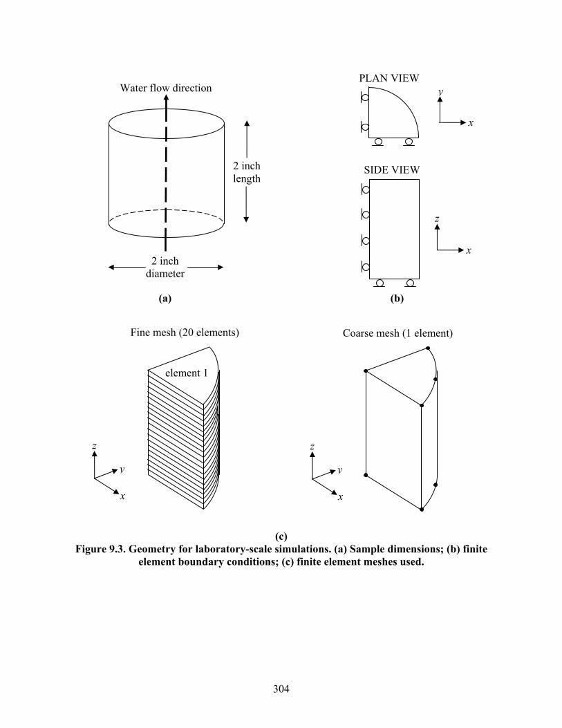
PLAN VIEW Water flow direction y
x
2 inch length
SIDE VIEW
z
x2 inch
diameter
(a) (b)
Fine mesh (20 elements) Coarse mesh (1 element)
element 1
z z
y y
x x
(c)
Figure 9.3. Geometry for laboratory-scale simulations. (a) Sample dimensions; (b) finite element boundary conditions; (c) finite element meshes used.
304

PLAN VIEW
1 mQuarter section y
evaluatedx
80 m0.8 m
80 m SIDE VIEW zz y
xx
(a) (b)
0
10
20
30
40
0 10 20 30x
y
40
(c)
Figure 9.4. Geometry for borehole-scale simulations. (a) Dimensions of region evaluated;
(b) finite element boundary conditions; (c) finite element mesh used.
305

PLAN VIEW
Quarter-sectionEkofisk field evaluated 3.6 km y
9.3 km x
6.9 km 26 km
Reservoir depth: 3.0-3.25 kmSIDE VIEW z
20 km x
z y (North)
x (East)
(a) (b)
13000 10000
z x y
Layer Thickness (m) Material 00 1-4 700 (each) Shale overburden Ekofisk
field 5 200 Shale overburden 6 120 Chalk (Ekofisk Fm.) 7 20 Chalk (tight zone) 8 110 Chalk (Tor Fm.) 9 350 Shale underburden
(c) Figure 9.5. Geometry for field-scale simulations. (a) Dimensions of region evaluated; (b)
finite element boundary conditions; (c) finite element mesh used.
306

Water flow direction
Strain gauge 4: element 3
Figure 9.6. Positions of “strain gauges” for the laboratory-scale simulations. These are the
local intervals over which strain is averaged and presented in Figures 9.7, 9.8, and 9.11. Results are also presented for average strain over the entire sample, which is equal to
displacement of the top of the sample divided by the sample length.
2 inch diameter
2 inch length Strain gauge 3: element 8
Positioned 1.7-1.8 inches above bottom
Positioned 1.2-1.3 inches above bottom Strain gauge 2: element 13
Strain gauge 1: element 18 Positioned 0.7-0.8 inches above bottom
Positioned 0.2-0.3 inches above bottom
307

0.0%0.2%0.4%0.6%0.8%1.0%1.2%1.4%1.6%1.8%2.0%2.2%2.4%2.6%2.8%3.0%
0.0 0.5 1.0 1.5 2.0 2.5Time (hours)
Axi
al S
trai
n ε z
gauge 4gauge 2 gauge 3gauge 1
Average strain
over full sample length
(a)
0.00%
0.02%
0.04%
0.06%
0.08%
0.10%
0.12%
0.0 0.5 1.0Time (ho
Rad
ial S
trai
n ε x
gauge 1 3gauge 2
(b) Figure 9.7. Strain histories at various localized inunder near-K0 stress conditions. For both (a) axia
occurs in a short time when the pore fluid changes fare much greater than radial strains for these stre
308
gauge
1.5 2.0 2.5urs)
gauge 4
tervals for a “fast” waterflooding test l strains and (b) radial strains, strain rom oil to water. Note that axial strains ss conditions. Compare to Figure 9.8.

-0.2%
0.0%
0.2%
0.4%
0.6%
0.8%
1.0%
1.2%
1.4%
0.0 0.5 1.0 1.5 2.0 2.5
Time (hours)
Axi
al S
trai
n ε z
gauge 4gauge 2 gauge 3gauge 1
Average strain
over full sample length
(a)
0.0%
0.1%
0.2%
0.3%
0.4%
0.5%
0.6%
0.7%
0.8%
0.9%
0.0 0.5 1.0 1.5 2.0 2.5Time (hours)
Rad
ial S
trai
n ε x
gauge 1 gauge 2 gauge 3 gauge 4
(b) Figure 9.8. Strain histories at various localized intervals for a “fast” waterflooding test
under hydrostatic stress conditions. For both (a) axial strains and (b) radial strains, strain occurs in a short time when the pore fluid changes from oil to water. Axial strains are only
slightly greater than radial strains for these stress conditions. Compare to Figure 9.7.
309

0.0
0.2
0.4
0.6
0.8
1.0
1.2
1.4
1.6
1.8
2.0
0.67 0.68 0.69
Posi
tion
in s
peci
men
(inc
hes)
Top of sample
t = 2 hours
s
Figure 9.9. History of void space distribunear-K0 stress conditions. Void ratio in any i
fluid changes
0.0
0.2
0.4
0.6
0.8
1.0
1.2
1.4
1.6
1.8
2.0
0.67 0.68 0.69
Posi
tion
in s
peci
men
(inc
hes)
Figure 9.10. History of void space distribuhydrostatic stress conditions. Void ratio in a
pore fluid chang
t = 1.75 hour
0.70 0.71 0.72 0.7Void ratio
Direction of w
ater flow
t = 1.5 hours
t = 1.25 hours
t = 1 hour
t = 0.75 hours
t = 0 hours
t = 0.5 hours
t = 0.25 hourse
tion during a “fast” waterflnterval decreases in a shorfrom oil to water.
0.70 0.71 0.72 0.7Void ratio
t = 2 hours
t = 1.5 hours
t = 1.25 hours
t = 1 hour
t = 0.75 hours
t = 0 hours
t = 0.5 hours
t = 0.25 hours
tion during a “fast” waterfny interval decreases in a
es from oil to water.
310
Bottom of sampl
3ooding test under t time when the pore
Top of sample
t = 1.75 hours
3
Direction of w
ater flow
e
s
Bottom of sampl
looding test under hort time when the

0.0%
0.5%
1.0%
1.5%
2.0%
2.5%
3.0%
3.5%
0 50 100 150 200 250 300 350 400 450Time (hours)
Axi
al S
trai
n ε z
Creep(oil saturated)
Creep(water saturated)
Wat
erflo
odin
g
gauge 1gauge 2gauge 3gauge 4
(a)
0.00%
0.05%
0.10%
0.15%
0.20%
0.25%
0.30%
0.35%
0.40%
0.45%
0 50 100 150 200 250 300 350 400 450Time (hours)
Rad
ial S
trai
n ε x
Creep(oil saturated)
Creep(water saturated)
Wat
erflo
odin
g
gauge 1gauge 2gauge 3gauge 4
(b) Figure 9.11. Strain histories at various localized intervals for a “slow” waterflooding test
simulation under near-K0 stress conditions, for a 20-element mesh. For both (a) axial strains and (b) radial strains, strain occurs in a short time when the pore fluid changes
from oil to water. Axial strains are much greater than radial strains for near-K0 conditions.
311

0.0%
0.5%
1.0%
1.5%
2.0%
2.5%
3.0%
3.5%
0 50 100 150 200 250 300 350 400 450Time (hours)
Axi
al, R
adia
l Str
ain ε z
, εx
Axial
Radial
Creep(oil saturated)
Creep(water saturated)
Wat
erflo
odin
g
Figure 9.12. Strain histories for a “slow” waterflooding test simulation under near-K0 stress conditions, for a 1-element mesh. Strain occurs in a short time when the pore fluid changes from oil to water. Axial strains are much greater than radial strains for near-K0 conditions.
0.0
0.2
0.4
0.6
0.8
1.0
1.2
1.4
1.6
1.8
2.0
0.65 0.66 0.67 0.68 0.69 0.70 0.71 0.72 0.73Void ratio
Posi
tion
in s
peci
men
(inc
hes)
Top of sample
t = 2hours
t = 250 hours
t = 210 t = 220 hours
00 hours
Direction of w
ater flowt = 400 hours
t = 190 hours
t = 180 hours
t = 30 hours
t = 0 hours
B e
Figure 9.13. History of void space distribution during a “slow” watsimulation under near-K0 stress conditions, for a 20-element mesh. Mor
space distribution is seen than for “fast” waterflooding test; compa
312
ottom of sampl
erflooding test e variability in void re to Figure 9.9.

0.0%
0.5%
1.0%
1.5%
2.0%
2.5%
3.0%
3.5%
0 50 100 150 200 250 300 350 400Time (hours)
Axi
al, R
adia
l Str
ain ε z
, εx
1-element mesh1-element meshDiscretized meshDiscretized mesh
radial strain
axial strain
Figure 9.14. Comparison of average strain histories for a “slow” waterflooding test simulation under near-K0 stress conditions, for a 1-element mesh and a 20-element mesh.
The average strains in each sample are nearly identical, indicating that the procedure used to calculate average properties of chalk in an element with variability in pore fluid
composition yields good results.
0
5
10
15
20
25
30
0 10 20 30 4Distance from center of borehole (m)
Effe
ctiv
e st
ress
(MPa
)
0
vertical stresstangential stress
radial stress
Figure 9.15. Stress distributions at the end of the simulation for the case in which waterflooding causes material weakening only.
313

0
5
10
15
20
25
30
0 10 20 30 40Distance from center of borehole (m)
Effe
ctiv
e st
ress
, por
e pr
essu
re (M
Pa) vertical stress
tangential stress
radial stress
pore presure
Figure 9.16. Stress distributions at the end of the simulation for the case in which waterflooding causes pore pressure increase only.
0
5
10
15
20
25
30
0 10 20 30 4Distance from center of borehole (m)
Effe
ctiv
e st
ress
, por
e pr
essu
re (M
Pa)
0
vertical stress
radial stress
tangential stress
pore presure
Figure 9.17. Stress distributions at the end of the simulation for the case in which waterflooding causes both pore pressure increase and material weakening.
314

0
2
4
6
8
10
12
14
16
18
0 1Distan
Rad
ial e
ffect
ive
stre
ss (M
Pa)
material weakening onlypore pressure increase only
m p
Figure 9.18. Comparison of radial waterfloo
0
2
4
6
8
10
12
14
16
18
0 1Distan
Tang
entia
l effe
ctiv
e st
ress
(MPa
)
Figure 9.19. Comparison of tangentiwaterfloo
aterial weakening andore pressure increase
0 20 30 40ce from center of borehole (m)
stress distributions for three simulations in which ding has different effects.
0
material weakening onlypore pressure increase only
m p
ad
aterial weakening andore pressure increase
20 30ce from center of borehole (m)
40
l stress distributions for three simulations in which ing has different effects.
315

0
5
10
15
20
25
30
0Dista
Vert
ical
effe
ctiv
e st
ress
(MPa
) pore pressure increase only
material weakening only
Figure 9.20. Comparison of verticawaterfloo
material weakening andpore pressure increase
10 20 30 4nce from center of borehole (m)
0
l stress distributions for three simulations in which ding has different effects.
316

-8
-7
-6
-5
-4
-3
-2
-1
0
1
0 5000 10000 15000North-South Distance (m)
Subs
iden
ce (m
)
Subsidence
Compaction
Reservoir Sideburden
(a)
-8
-7
-6
-5
-4
-3
-2
-1
0
1
0 2000 4000 6000 8000 10000East-West Distance (m)
Subs
iden
ce (m
)
Subsidence
Compaction
Reservoir Sideburden
(b)
Figure 9.21. Compaction and subsidence profiles for the Ekofisk field for the case without water-weakening. Profiles are shown for (a) north-south direction; (b) east-west direction.
317

-8
-7
-6
-5
-4
-3
-2
-1
0
0 5 10 15 20 25 30Pressure drawdown (MPa)
Subs
iden
ce (m
)
Subsidence at centerCompaction at center
Figure 9.22. Compaction and subsidence history for the Ekofisk field for the case without water-weakening.
318

-10
-8
-6
-4
-2
0
2
0 5000 10000 15000North-South Distance (m)
Subs
iden
ce (m
)
Subsidence
Compaction
Reservoir Sideburden
(a)
-10
-8
-6
-4
-2
0
2
0 2000 4000 6000 8000 10000East-West Distance (m)
Subs
iden
ce (m
)
Subsidence
Compaction
Reservoir Sideburden
(b)
Figure 9.23. Compaction and subsidence profiles for the Ekofisk field for the case with water-weakening. Profiles are shown for (a) north-south direction; (b) east-west direction.
319

-10
-9
-8
-7
-6
-5
-4
-3
-2
-1
0
0 5 10 15 20 25 30Pressure drawdown (MPa)
Subs
iden
ce (m
)
Subsidence at centerCompaction at center
Figure 9.24. Compaction and subsidence history for the Ekofisk field for the case with water-weakening.
320