41

Chapter 9 - Mechanics of Options Markets • Types of options • Option positions and profit/loss diagrams • Underlying assets • Specifications • Trading options • Margins • Taxation • Warrants, employee stock options, and convertibles • Types of options

Two types of options: call options vs. put options Four positions: buy a call, sell (write) a call, buy a put, sell (write) a put

• Option positions and profit/loss diagrams

Notations S0: the current price of the underlying asset K: the exercised (strike) price T: the time to expiration of option ST: the price of the underlying asset at time T C: the call price (premium) of an American option c: the call price (premium) of a European option P: the put price (premium) of an American option p: the put price (premium) of a European option r: the risk-free interest rate σ : the volatility (standard deviation) of the underlying asset price

(1) Buy a European call option: buy a June 90 call option at $2.50

Stock price at expiration 0 70 90 110

Buy June 90 call @ $2.50 -2.50 -2.50 -2.50 17.50 Net cost $2.50 -2.50 -2.50 -2.50 17.50

Profit / loss Maximum gain

unlimited

Stock price Max loss

42

Write a European call option: write a June 90 call at $2.50 (exercise for students, reverse the above example) Buy a European put option: buy a July 85 put at $2.00

Stock price at expiration 0 65 85 105

Buy June 85 put @ $2.00 83.00 18.00 -2.00 -2.00 Net cost $2.00 83.00 18.00 -2.00 -2.00

Profit / loss Max gain Stock price Max loss

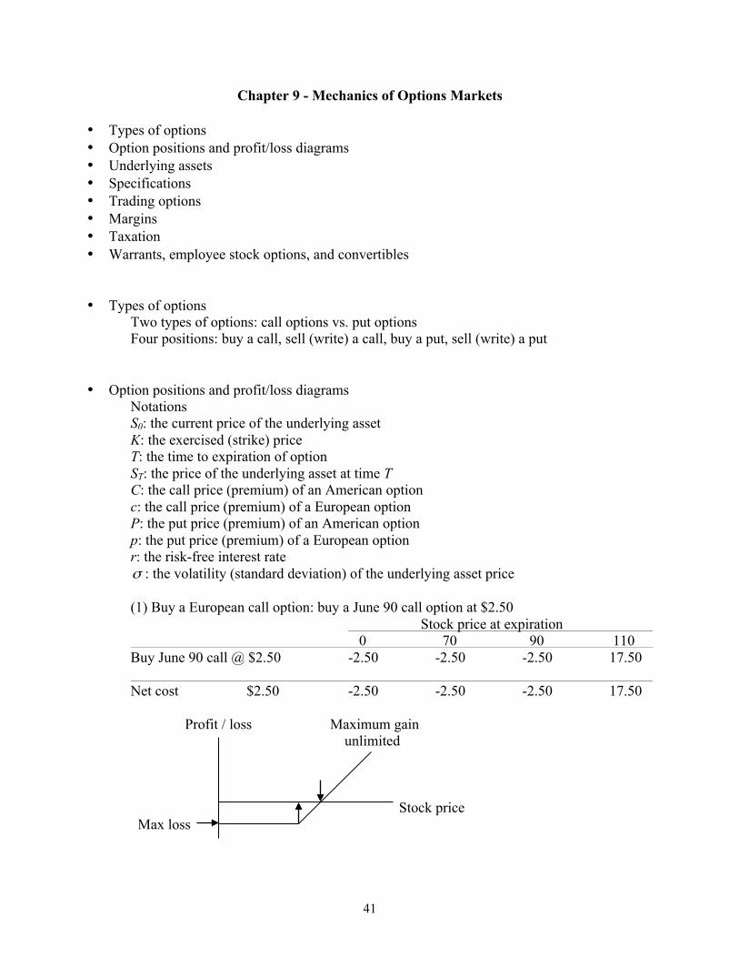
Write a European put option: write a July 85 put at $2.00 (exercise for students, reverse the above example) In general, the payoff at time T: (1) For a long European call option is = max (ST - K, 0) (2) For a short European call option is = min (K - ST, 0) = -max (ST - K, 0) (3) For a long European put option is = max (K - ST, 0) (4) For a short European put option is = min (ST - K, 0) = -max (K - ST, 0) Payoff Payoff Payoff Payoff

K ST ST ST K K ST K

(1) (2) (3) (4) In-the-money options: S > K for calls and S < K for puts Out-of-the-money options: S < K for calls and S > K for puts At-the-money options: S = K for both calls and puts

43

Intrinsic value = max (S - K, 0) for a call option Intrinsic value = max (K - S, 0) for a put option C (or P) = intrinsic value + time value

Suppose a June 85 call option sells for $2.50 and the market price of the stock is $86, then the intrinsic value = 86 – 85 = $1; time value = 2.50 - 1 = $1.50 Suppose a June 85 put option sells for $1.00 and the market price of the stock is $86, then the intrinsic value = 0; time value = 1 - 0 = $1 Naked call option writing: the process of writing a call option on a stock that the option writer does not own

Naked options vs. covered options • Underlying assets

If underlying assets are stocks - stock options If underlying assets are foreign currencies - currency options If underlying assets are stock indexes - stock index options If underlying assets are commodity futures contracts - futures options If the underlying assets are futures on fixed income securities (T-bonds, T-notes) - interest-rate options

• Specifications Dividends and stock splits: exchange-traded options are not adjusted for cash dividends but are adjusted for stock splits Position limits: the CBOE specifies a position limit for each stock on which options are traded. There is an exercise limit as well (equal to position limit) Expiration date: the third Friday of the month

• Trading options

Market maker system (specialist) and floor broker Offsetting orders: by issuing an offsetting order Bid-offer spread Commissions

44

• Margins Writing naked options are subject to margin requirements The initial margin for writing a naked call option is the greater of (1) A total of 100% of proceeds plus 20% of the underlying share price less the amount, if any, by which the option is out of the money (2) A total of 100% of proceeds plus 10% of the underlying share price The initial margin for writing a naked put option is the greater of (1) A total of 100% of proceeds plus 20% of the underlying share price less the amount, if any, by which the option is out of the money (2) A total of 100% of proceeds plus 10% of the exercise price For example, an investor writes four naked call options on a stock. The option price is $5, the exercise price is $40, and the stock price is $38. Because the option is $2 out of the money, the first calculation gives 400*(5+0.2*38-2) = $4,240 while the second calculation gives 400*(5+0.1*38) = $3,520. So the initial margin is $4,240. If the options were puts, it would be $2 in the money. The initial margin from the first calculation would be 400*(5+0.2*38) = $5,040 while it would be 400*(5+0.1*40) = $3,600 from the second calculation. So the initial margin would be $5,040. Buying options requires cash payments and there are no margin requirements Writing covered options are not subject to margin requirements (stocks as collateral)

• Taxation

In general, gains or losses are taxed as capital gains or losses. If the option is exercised, the gain or loss from the option is rolled over to the position taken in the stock.

Wash sale rule: when the repurchase is within 30 days of the sale, the loss on the sale is not tax deductible

• Warrants, employee stock options, and convertibles

Warrants are options issued by a financial institution or a non-financial corporation. Employee stock options are call options issued to executives by their company to motivate them to act in the best interest of the company’s shareholders. Convertible bonds are bonds issued by a company that can be converted into common stocks.

• Assignments Quiz (required) Practice Questions: 9.9, 9.10 and 9.12

45

Chapter 10 - Properties of Stock Options • Factors affecting option prices • Upper and lower bounds for option prices • Put-call parity • Early exercise • Effect of dividends • Factors affecting option prices

Six factors: Current stock price, S0 Strike (exercise) price, K Time to expiration, T Volatility of the stock price, σ Risk-free interest rate, r Dividends expected during the life of the option

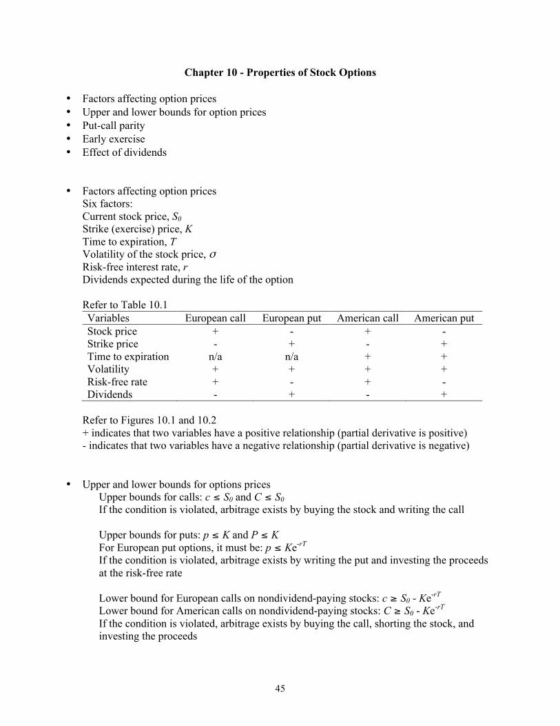
Refer to Table 10.1

Variables European call European put American call American put Stock price + - + - Strike price - + - + Time to expiration n/a n/a + + Volatility + + + + Risk-free rate + - + - Dividends - + - +

Refer to Figures 10.1 and 10.2

+ indicates that two variables have a positive relationship (partial derivative is positive) - indicates that two variables have a negative relationship (partial derivative is negative)

• Upper and lower bounds for options prices Upper bounds for calls: c ≤ S0 and C ≤ S0

If the condition is violated, arbitrage exists by buying the stock and writing the call

Upper bounds for puts: p ≤ K and P ≤ K For European put options, it must be: p ≤ Ke-rT If the condition is violated, arbitrage exists by writing the put and investing the proceeds at the risk-free rate Lower bound for European calls on nondividend-paying stocks: c ≥ S0 - Ke-rT Lower bound for American calls on nondividend-paying stocks: C ≥ S0 - Ke-rT If the condition is violated, arbitrage exists by buying the call, shorting the stock, and investing the proceeds

46

Lower bound for European puts on nondividend-paying stocks: p ≥ Ke-rT - S0 Lower bound for American puts on nondividend-paying stocks: P ≥ K - S0 If violated, arbitrage exists by borrowing money and buying the put and the stock

• Put -call parity

Considers the relationship between p and c written on the same stock with same exercise price and same maturity date

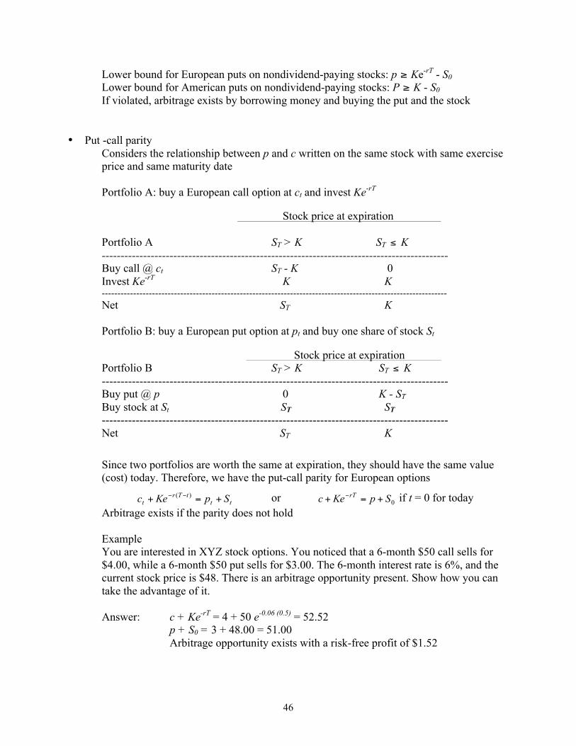
Portfolio A: buy a European call option at ct and invest Ke-rT

Stock price at expiration

Portfolio A ST > K ST ≤ K -------------------------------------------------------------------------------------------- Buy call @ ct ST - K 0 Invest Ke-rT K K -------------------------------------------------------------------------------------------------------------- Net ST K Portfolio B: buy a European put option at pt and buy one share of stock St

Stock price at expiration Portfolio B ST > K ST ≤ K -------------------------------------------------------------------------------------------- Buy put @ p 0 K - ST Buy stock at St

ST ST --------------------------------------------------------------------------------------------

Net ST K

Since two portfolios are worth the same at expiration, they should have the same value (cost) today. Therefore, we have the put-call parity for European options

tttTr

t SpKec +=+ −− )( or 0SpKec rT +=+ − if t = 0 for today Arbitrage exists if the parity does not hold Example You are interested in XYZ stock options. You noticed that a 6-month $50 call sells for $4.00, while a 6-month $50 put sells for $3.00. The 6-month interest rate is 6%, and the current stock price is $48. There is an arbitrage opportunity present. Show how you can take the advantage of it.

Answer: c + Ke-rT = 4 + 50 e-0.06 (0.5) = 52.52

p + S0 = 3 + 48.00 = 51.00 Arbitrage opportunity exists with a risk-free profit of $1.52

47

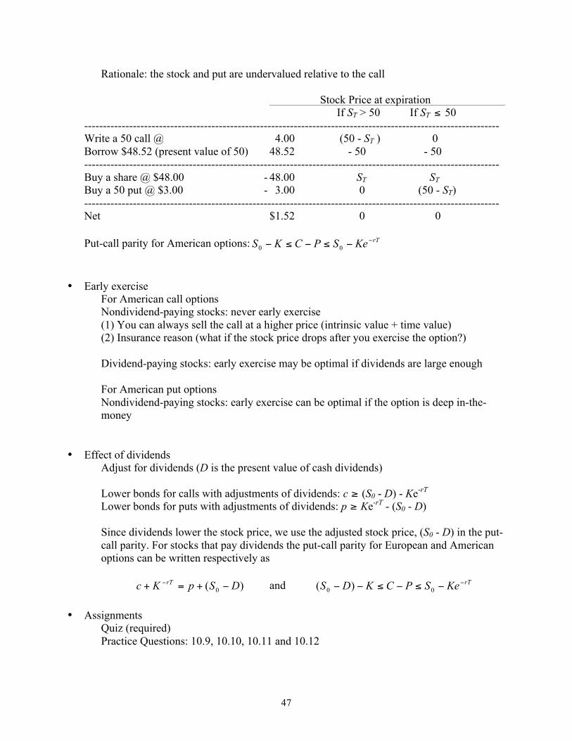
Rationale: the stock and put are undervalued relative to the call Stock Price at expiration If ST > 50 If ST ≤ 50 --------------------------------------------------------------------------------------------------------------- Write a 50 call @ 4.00 (50 - ST ) 0 Borrow $48.52 (present value of 50) 48.52 - 50 - 50 --------------------------------------------------------------------------------------------------------------- Buy a share @ $48.00 - 48.00 ST ST Buy a 50 put @ $3.00 - 3.00 0 (50 - ST) ---------------------------------------------------------------------------------------------------------------

Net $1.52 0 0

Put-call parity for American options: rTKeSPCKS −−≤−≤− 00 • Early exercise For American call options Nondividend-paying stocks: never early exercise

(1) You can always sell the call at a higher price (intrinsic value + time value) (2) Insurance reason (what if the stock price drops after you exercise the option?)

Dividend-paying stocks: early exercise may be optimal if dividends are large enough

For American put options

Nondividend-paying stocks: early exercise can be optimal if the option is deep in-the-money

• Effect of dividends Adjust for dividends (D is the present value of cash dividends) Lower bonds for calls with adjustments of dividends: c ≥ (S0 - D) - Ke-rT

Lower bonds for puts with adjustments of dividends: p ≥ Ke-rT - (S0 - D)

Since dividends lower the stock price, we use the adjusted stock price, (S0 - D) in the put-call parity. For stocks that pay dividends the put-call parity for European and American options can be written respectively as

)( 0 DSpKc rT −+=+ − and rTKeSPCKDS −−≤−≤−− 00 )( • Assignments

Quiz (required) Practice Questions: 10.9, 10.10, 10.11 and 10.12

48

Chapter 11 - Trading Strategies Involving Options • Strategies with a single option and a stock • Spreads • Combinations • Strategies with a single option and a stock

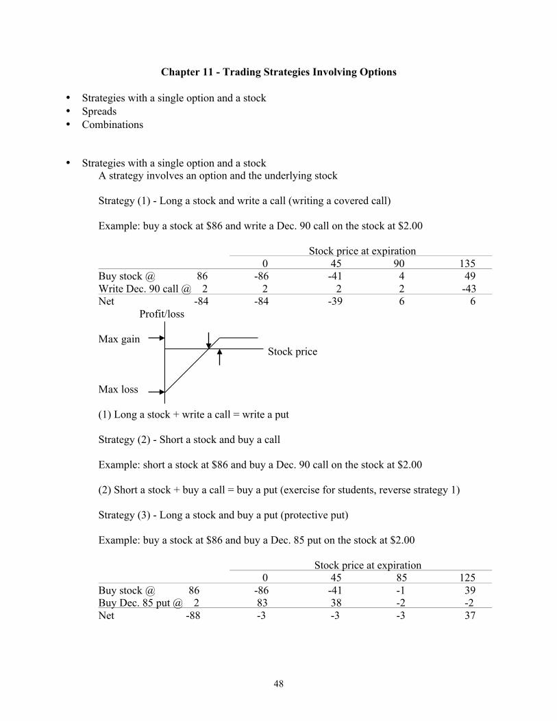
A strategy involves an option and the underlying stock Strategy (1) - Long a stock and write a call (writing a covered call) Example: buy a stock at $86 and write a Dec. 90 call on the stock at $2.00

Stock price at expiration

0 45 90 135 Buy stock @ 86 -86 -41 4 49 Write Dec. 90 call @ 2 2 2 2 -43 Net -84 -84 -39 6 6

Profit/loss Max gain Stock price Max loss

(1) Long a stock + write a call = write a put

Strategy (2) - Short a stock and buy a call Example: short a stock at $86 and buy a Dec. 90 call on the stock at $2.00 (2) Short a stock + buy a call = buy a put (exercise for students, reverse strategy 1)

Strategy (3) - Long a stock and buy a put (protective put) Example: buy a stock at $86 and buy a Dec. 85 put on the stock at $2.00

Stock price at expiration 0 45 85 125

Buy stock @ 86 -86 -41 -1 39 Buy Dec. 85 put @ 2 83 38 -2 -2 Net -88 -3 -3 -3 37

49

Profit/loss Max gain Stock price Max loss

(3) Long a stock + buy a put = buy a call Strategy (4) - Short a stock and write a put Example: short a stock at $86 and write a Dec. 85 put on the stock at $2.00 (4) Short a stock + write a put = write a call (exercise for students, reverse strategy 3)

• Spreads

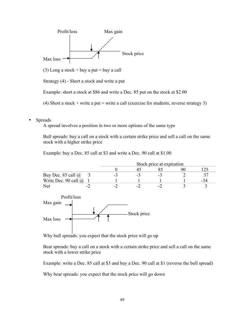
A spread involves a position in two or more options of the same type Bull spreads: buy a call on a stock with a certain strike price and sell a call on the same stock with a higher strike price

Example: buy a Dec. 85 call at $3 and write a Dec. 90 call at $1.00

Stock price at expiration

0 45 85 90 125 Buy Dec. 85 call @ 3 -3 -3 -3 2 37 Write Dec. 90 call @ 1 1 1 1 1 -34 Net -2 -2 -2 -2 3 3

Profit/loss Max gain Stock price Max loss Why bull spreads: you expect that the stock price will go up Bear spreads: buy a call on a stock with a certain strike price and sell a call on the same stock with a lower strike price Example: write a Dec. 85 call at $3 and buy a Dec. 90 call at $1 (reverse the bull spread) Why bear spreads: you expect that the stock price will go down

50

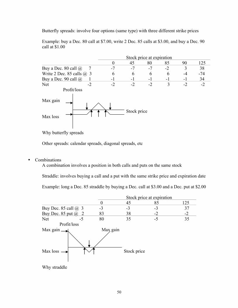
Butterfly spreads: involve four options (same type) with three different strike prices Example: buy a Dec. 80 call at $7.00, write 2 Dec. 85 calls at $3.00, and buy a Dec. 90 call at $1.00

Stock price at expiration 0 45 80 85 90 125

Buy a Dec. 80 call @ 7 -7 -7 -7 -2 3 38 Write 2 Dec. 85 calls @ 3 6 6 6 6 -4 -74 Buy a Dec. 90 call @ 1 -1 -1 -1 -1 -1 34

Net -2 -2 -2 -2 3 -2 -2 Profit/loss Max gain Stock price Max loss Why butterfly spreads

Other spreads: calendar spreads, diagonal spreads, etc

• Combinations A combination involves a position in both calls and puts on the same stock Straddle: involves buying a call and a put with the same strike price and expiration date

Example: long a Dec. 85 straddle by buying a Dec. call at $3.00 and a Dec. put at $2.00 Stock price at expiration 0 45 85 125

Buy Dec. 85 call @ 3 -3 -3 -3 37 Buy Dec. 85 put @ 2 83 38 -2 -2 Net -5 80 35 -5 35

Profit/loss Max gain Max gain Max loss Stock price Why straddle

51

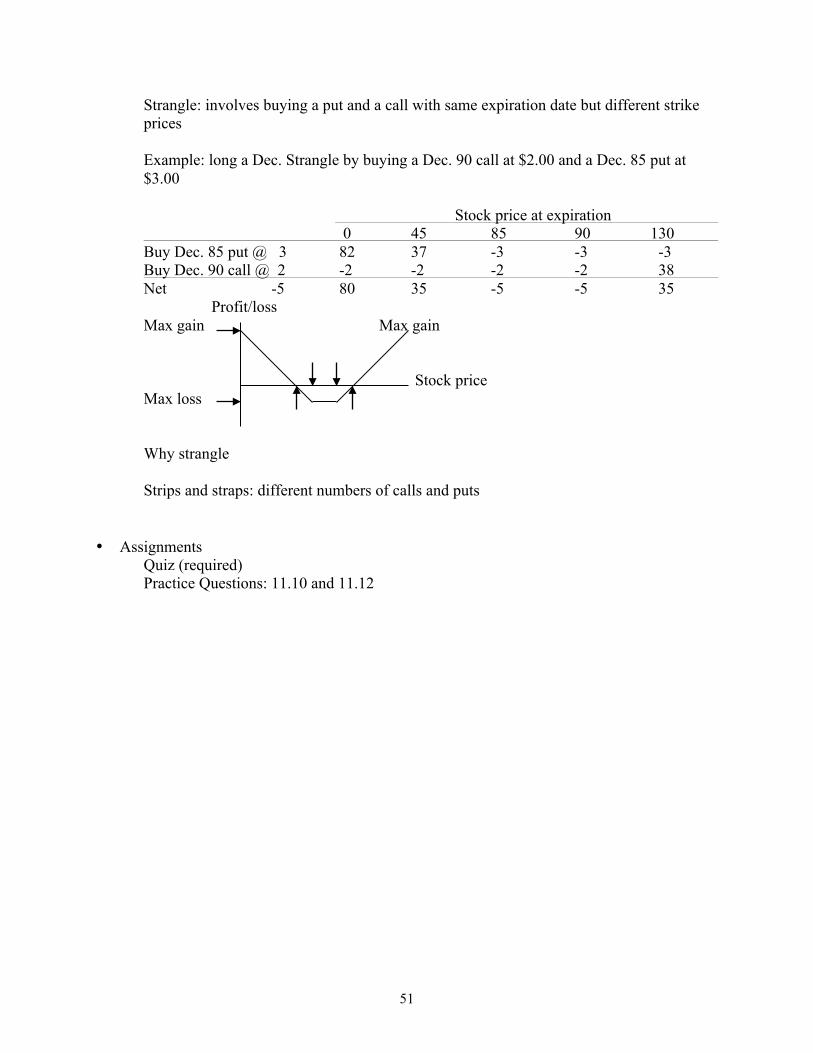
Strangle: involves buying a put and a call with same expiration date but different strike prices Example: long a Dec. Strangle by buying a Dec. 90 call at $2.00 and a Dec. 85 put at $3.00

Stock price at expiration

0 45 85 90 130 Buy Dec. 85 put @ 3 82 37 -3 -3 -3 Buy Dec. 90 call @ 2 -2 -2 -2 -2 38 Net -5 80 35 -5 -5 35

Profit/loss Max gain Max gain Stock price Max loss Why strangle Strips and straps: different numbers of calls and puts • Assignments

Quiz (required) Practice Questions: 11.10 and 11.12

52

Chapter 12 - Binomial Option Pricing Model • A one-step binomial model • Risk-neutral valuation • Two-step binomial model • Matching volatility with u and d • Options on other assets • One-step binomial model

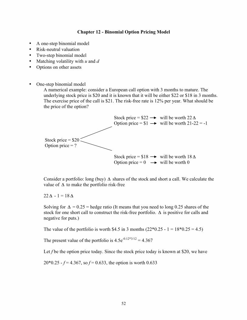
A numerical example: consider a European call option with 3 months to mature. The underlying stock price is $20 and it is known that it will be either $22 or $18 in 3 months. The exercise price of the call is $21. The risk-free rate is 12% per year. What should be the price of the option?

Stock price = $22 will be worth 22Δ Option price = $1 will be worth 21-22 = -1 Stock price = $20 Option price = ? Stock price = $18 will be worth 18Δ Option price = 0 will be worth 0

Consider a portfolio: long (buy) Δ shares of the stock and short a call. We calculate the value of Δ to make the portfolio risk-free 22Δ - 1 = 18Δ

Solving for Δ = 0.25 = hedge ratio (It means that you need to long 0.25 shares of the stock for one short call to construct the risk-free portfolio. Δ is positive for calls and negative for puts.)

The value of the portfolio is worth $4.5 in 3 months (22*0.25 - 1 = 18*0.25 = 4.5) The present value of the portfolio is 4.5e-0.12*3/12 = 4.367 Let f be the option price today. Since the stock price today is known at $20, we have

20*0.25 - f = 4.367, so f = 0.633, the option is worth 0.633

53

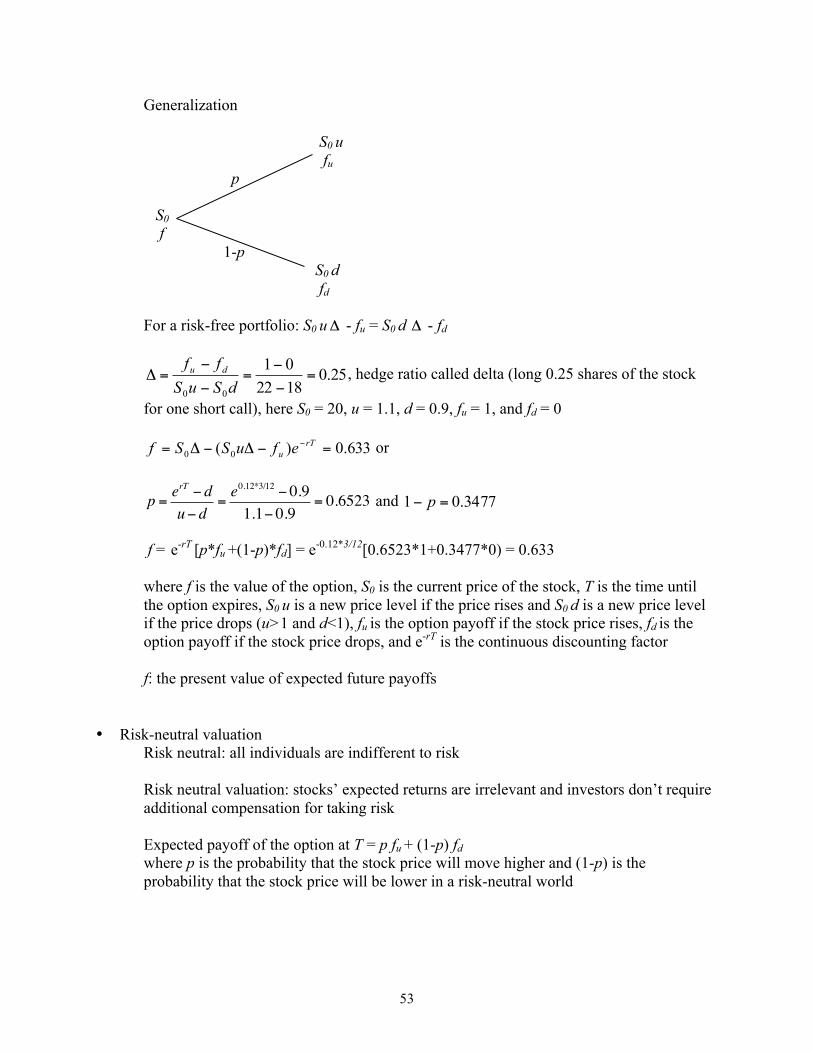
Generalization S0 u fu p S0 f 1-p S0 d fd For a risk-free portfolio: S0 uΔ - fu = S0 d Δ - fd

25.0182201

00

=−

−=

−

−=Δ

dSuSff du , hedge ratio called delta (long 0.25 shares of the stock

for one short call), here S0 = 20, u = 1.1, d = 0.9, fu = 1, and fd = 0

633.0)( 00 =−Δ−Δ= −rTu efuSSf or

p = erT − du− d

=e0.12*3/12 − 0.91.1− 0.9

= 0.6523 and 3477.01 =− p

f = e-rT [p*fu +(1-p)*fd] = e-0.12*3/12[0.6523*1+0.3477*0) = 0.633 where f is the value of the option, S0 is the current price of the stock, T is the time until the option expires, S0 u is a new price level if the price rises and S0 d is a new price level if the price drops (u>1 and d<1), fu is the option payoff if the stock price rises, fd is the option payoff if the stock price drops, and e-rT is the continuous discounting factor

f: the present value of expected future payoffs • Risk-neutral valuation

Risk neutral: all individuals are indifferent to risk Risk neutral valuation: stocks’ expected returns are irrelevant and investors don’t require additional compensation for taking risk

Expected payoff of the option at T = p fu + (1-p) fd where p is the probability that the stock price will move higher and (1-p) is the probability that the stock price will be lower in a risk-neutral world

54

Expected stock price at T = E(ST) = p(S0 u) + (1-p)(S0 d) = S0 erT Stock price grows on average at the risk-free rate. The expected return on all securities is the risk-free rate. Real world vs. risk-neutral world In the about numerical example, we assume that the risk-free rate is 12% per year. We have p = 0.6523 and 1-p = 0.3477. The option price is 0.633. What would happen if the expected rate of return on the stock is 16% (r*) in the real world? Let p* be the probability of an up movement in stock price, the expected stock price at T must satisfy the following condition: 22p* + 18(1-p*) = 20 e0.16*3/12, solving for p* = 0.7041 and 1-p* = 0.2959 f = e-r*T [(p*)*fu +(1-p*)*fd] = e-0.16*3/12[0.7041*1+0.2959*0] = 0.676 Note: in the real world, it is difficult to determine the appropriate discount rate to price options since options are riskier than stocks

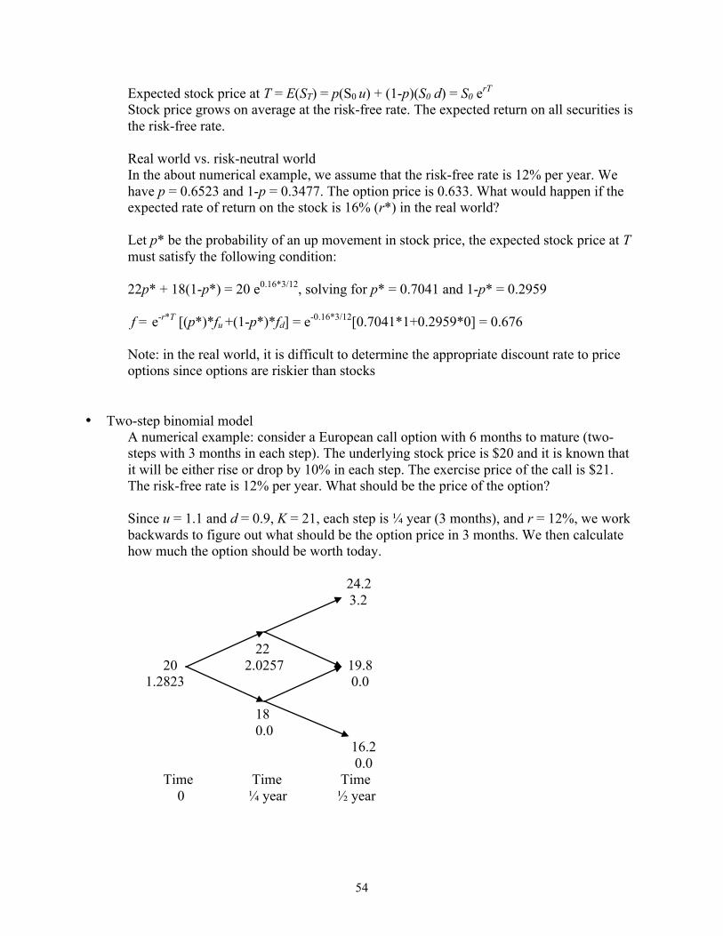
• Two-step binomial model A numerical example: consider a European call option with 6 months to mature (two-steps with 3 months in each step). The underlying stock price is $20 and it is known that it will be either rise or drop by 10% in each step. The exercise price of the call is $21. The risk-free rate is 12% per year. What should be the price of the option?

Since u = 1.1 and d = 0.9, K = 21, each step is ¼ year (3 months), and r = 12%, we work backwards to figure out what should be the option price in 3 months. We then calculate how much the option should be worth today.

24.2 3.2 22 20 2.0257 19.8 1.2823 0.0 18 0.0 16.2 0.0 Time Time Time

0 ¼ year ½ year

55

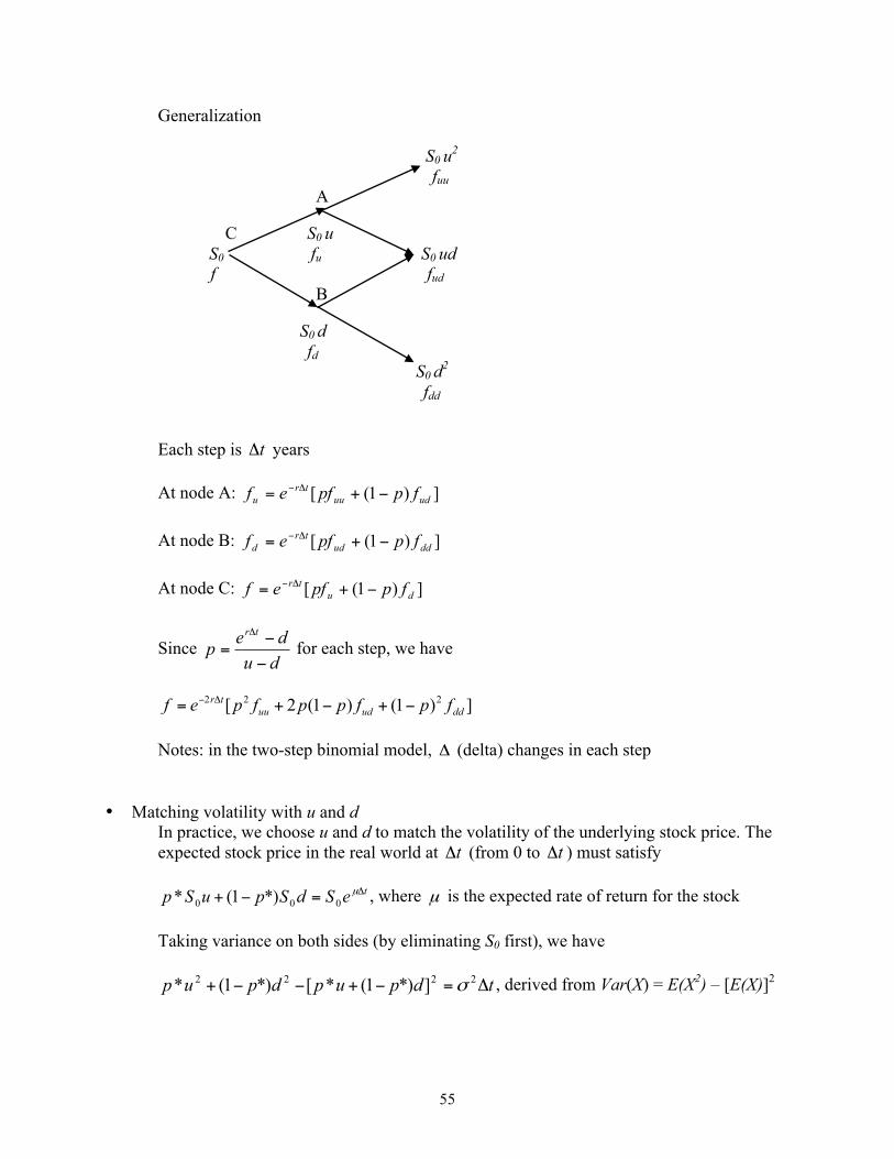
Generalization

S0 u2 fuu A C S0 u S0 fu S0 ud f fud B S0 d fd S0 d2 fdd Each step is tΔ years At node A: ])1([ uduu

tru fppfef −+= Δ−

At node B: ])1([ ddud

trd fppfef −+= Δ−

At node C: ])1([ du

tr fppfef −+= Δ−

Since dudep

tr

−

−=

Δ

for each step, we have

])1()1(2[ 222

dduduutr fpfppfpef −+−+= Δ−

Notes: in the two-step binomial model, Δ (delta) changes in each step • Matching volatility with u and d

In practice, we choose u and d to match the volatility of the underlying stock price. The expected stock price in the real world at tΔ (from 0 to tΔ ) must satisfy

teSdSpuSp Δ=−+ µ000 *)1(* , where µ is the expected rate of return for the stock

Taking variance on both sides (by eliminating S0 first), we have

tdpupdpup Δ=−+−−+ 2222 ]*)1(*[*)1(* σ , derived from Var(X) = E(X2) – [E(X)]2

56

Substituting dudep

T

−

−=

Δµ

* into the above equation gives

teuddue tt Δ=−−+ ΔΔ 22)( σµµ Ignoring 2tΔ and higher powers of tΔ , one solution is

teu Δ= σ and ted Δ−= σ (volatility matching u and d) For example, consider an American put option. The current stock price is $50 and the exercise price is $52. The risk-free rate is 5% per year and the life of the option is 2 years. There are two steps ( tΔ = 1 year in this case). Suppose the volatility is 20% per year. Then

teu Δ= σ = 1.2214 and ted Δ−= σ = 0.8187 • Options on other assets

Binomial models can be used to price options on stocks paying a continuous dividend yield, on stock indices, on currencies, and on futures. To increase the number of steps, we use the software included in the textbook.

• Assignments Quiz (required) Practice Questions: 12.9 12.10, 12.11 and 12.12

57

Chapters 13 - Black-Scholes Option Pricing Model • Lognormal property of stock prices • Distribution of the rate of return • Volatility • Black-Scholes option pricing model • Risk-neutral valuation • Implied volatility • Dividends • Greek Letters • Extensions • Lognormal property of stock prices

If percentage changes in a stock price in a short period of time, tΔ , follow a normal distribution:

),(~ 2 ttSS

ΔΔΔ

σµφ , then between times 0 and T, it follows

],)2

[(~ln 22

0

TTSST σ

σµφ − and

],)2

([(ln~ln 22

0 TTSST σσ

µφ −+

Stock price follows a lognormal distribution

For example, consider a stock with an initial price of $40. The expected return is 16% per year and a volatility of 20%. The probability distribution of the stock price in 6 months (T = 0.5) is

)02.0,759.3(]5.02.0,5.0)22.016.0(40[ln~ln 22

φφ =−+TS

The 95% confidence interval (2 σ rule) is (3.759 - 1.96*0.141, 3.759 + 1.96*0.141), where 0.141 is the standard deviation ( 141.002.0 = ). Thus, there is a 95% probability that the stock price in 6 months will be (32.55, 56.56) 32.55 = e3.759-1.96*0.141 < TS < e3.759+1.96*0.141 = 56.56

The mean of ST = 43.33 and the variance of ST = 37.93 (using formula 13.3)

58

• Distribution of the rate of return If a stock price follows a lognormal distribution, then the stock return follows a normal distribution. Let R be the continuous compounded rate of return per year realized between times 0 and T, then

RTT eSS 0= or

0ln1SS

TR T= . Therefore, ),

2(~ln1

22

0 TSS

TR T σσ

µφ −=

For example, consider a stock with an expected return of 17% per year and a volatility of 20% per year. The probability distribution for the average rate of return (continuously compounding) over 3 years is normally distributed

)32.0,

22.017.0(~

22

−φR or )0133.0,15.0(~φR

i.e., the mean is 15% per year over 3 years and the standard deviation is 11.55% (

1155.00133.0 = ) • Volatility

Stocks typically have volatilities (standard deviation) between 15% and 50% per year. In a small interval, tΔ , tΔ2σ is approximately equal to the variance of the percentage change in the stock price. Therefore, tΔσ is the standard deviation of the percentage change in the stock price. For example, if 3.0%30 ==σ then the standard deviation of the percentage change in the stock price in 1 week is a approximately %16.452/1*30 = Estimating volatility from historical data (1) Collect price data, iS (daily, weekly, monthly, etc.) over time period τ (in years)

(2) Obtain returns )ln(1−

=i

ii S

Sµ

(3) Estimate standard deviation of iµ , which is s

(4) The estimated standard deviation in τ years is τ

σs

=∧

59

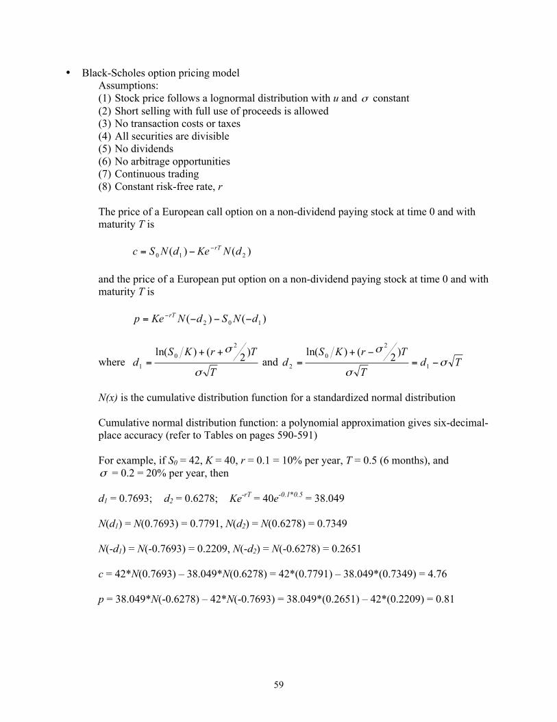
• Black-Scholes option pricing model Assumptions: (1) Stock price follows a lognormal distribution with u and σ constant (2) Short selling with full use of proceeds is allowed (3) No transaction costs or taxes (4) All securities are divisible (5) No dividends (6) No arbitrage opportunities (7) Continuous trading (8) Constant risk-free rate, r The price of a European call option on a non-dividend paying stock at time 0 and with maturity T is

)()( 210 dNKedNSc rT−−=

and the price of a European put option on a non-dividend paying stock at time 0 and with maturity T is

)()( 102 dNSdNKep rT −−−= −

where T

TrKSd

σ

σ )2()ln(2

01

++= and Td

T

TrKSd σ

σ

σ−=

−+= 1

2

02

)2()ln(

N(x) is the cumulative distribution function for a standardized normal distribution

Cumulative normal distribution function: a polynomial approximation gives six-decimal-place accuracy (refer to Tables on pages 590-591)

For example, if S0 = 42, K = 40, r = 0.1 = 10% per year, T = 0.5 (6 months), and σ = 0.2 = 20% per year, then

d1 = 0.7693; d2 = 0.6278; Ke-rT = 40e-0.1*0.5 = 38.049 N(d1) = N(0.7693) = 0.7791, N(d2) = N(0.6278) = 0.7349 N(-d1) = N(-0.7693) = 0.2209, N(-d2) = N(-0.6278) = 0.2651 c = 42*N(0.7693) – 38.049*N(0.6278) = 42*(0.7791) – 38.049*(0.7349) = 4.76 p = 38.049*N(-0.6278) – 42*N(-0.7693) = 38.049*(0.2651) – 42*(0.2209) = 0.81

60

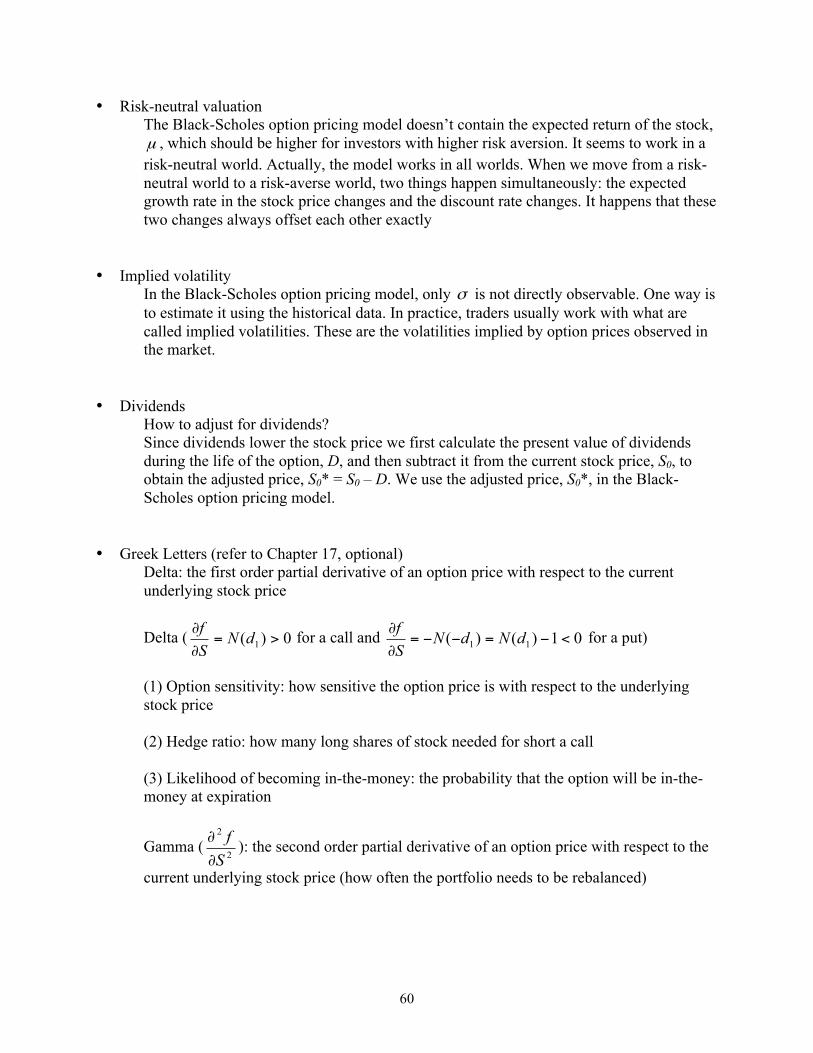
• Risk-neutral valuation The Black-Scholes option pricing model doesn’t contain the expected return of the stock, µ , which should be higher for investors with higher risk aversion. It seems to work in a risk-neutral world. Actually, the model works in all worlds. When we move from a risk-neutral world to a risk-averse world, two things happen simultaneously: the expected growth rate in the stock price changes and the discount rate changes. It happens that these two changes always offset each other exactly

• Implied volatility In the Black-Scholes option pricing model, only σ is not directly observable. One way is to estimate it using the historical data. In practice, traders usually work with what are called implied volatilities. These are the volatilities implied by option prices observed in the market.

• Dividends How to adjust for dividends?

Since dividends lower the stock price we first calculate the present value of dividends during the life of the option, D, and then subtract it from the current stock price, S0, to obtain the adjusted price, S0* = S0 – D. We use the adjusted price, S0*, in the Black-Scholes option pricing model.

• Greek Letters (refer to Chapter 17, optional) Delta: the first order partial derivative of an option price with respect to the current underlying stock price

Delta ( 0)( 1 >=∂

∂ dNSf for a call and 01)()( 11 <−=−−=

∂

∂ dNdNSf for a put)

(1) Option sensitivity: how sensitive the option price is with respect to the underlying stock price

(2) Hedge ratio: how many long shares of stock needed for short a call

(3) Likelihood of becoming in-the-money: the probability that the option will be in-the-money at expiration

Gamma (2

2

Sf

∂

∂ ): the second order partial derivative of an option price with respect to the

current underlying stock price (how often the portfolio needs to be rebalanced)

61

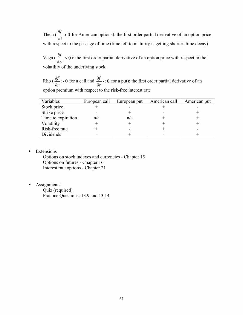
Theta ( 0<∂

∂

tf for American options): the first order partial derivative of an option price

with respect to the passage of time (time left to maturity is getting shorter, time decay)

Vega ( 0>∂

∂

σf ): the first order partial derivative of an option price with respect to the

volatility of the underlying stock

Rho ( 0>∂

∂

rf for a call and 0<

∂

∂

rf for a put): the first order partial derivative of an

option premium with respect to the risk-free interest rate

Variables European call European put American call American put Stock price + - + - Strike price - + - + Time to expiration n/a n/a + + Volatility + + + + Risk-free rate + - + - Dividends - + - +

• Extensions

Options on stock indexes and currencies - Chapter 15 Options on futures - Chapter 16

Interest rate options - Chapter 21 • Assignments

Quiz (required) Practice Questions: 13.9 and 13.14