Embed Size (px)
Citation preview

Geol. 656 Isotope Geochemistry
Chapter 9: Stable Isotopes at High Temperature
278 12/4/13
Stable Isotope Geochemistry II: High
Temperature Applications 9.1 INTRODUCTION
Stable isotopes have a number of uses in high temperature geochemistry (i.e., igneous and meta-morphic geochemistry). Perhaps the most important of these is geothermometry, i.e., deducing the temperatures at which mineral assemblages equilibrated. This application makes use of the tempera-ture dependency of fractionation factors. Other important applications include reconstructing ancient hydrothermal systems, detecting crustal assimilation in mantle-derived magmas, and tracing recycled crust in the mantle. These applications primarily involve O isotopes. Before discussing these subjects, let's briefly review the factors governing isotopic fractionation.
9.2 EQUILIBRIUM FRACTIONATIONS AMONG MINERALS In Chapter 8, we found that the translational and rotation contributions to the partition function do not vary with temperature. In our example calculation at low temperature, we found the vibrational contribution varies with the inverse of absolute temperature. At higher temperature, the e-hν/kT term in equation 8.35 becomes finite and this relationship breaks down and the equilibrium constant becomes proportional to the inverse square of temperature:
lnK = A +B
T 2 9.1
where A and B are constants. At infinite temperature, the fractionation is unity; i.e., ln K ≈ 0. Because of
Figure 9.1. a. Comparison of quartz-mineral fractionation factors estimated from the difference in oxygen site potential (Vqtz – Vmineral) and experimentally observed fractionation factors at 1000 K. b. Comparison of fractionation factors estimated through the increment method, which also considers cation mass, and experimentally observed fractionation factors at 1000 K. From Chacko, et al. (2001).
Geol. 656 Isotope Geochemistry
Chapter 9: Stable Isotopes at High Temperature
279 12/4/13
the nature of this temperature dependency, fractionation of stable isotopes at mantle temperatures will usually be small and stable isotopes can be used as tracers, particularly in crustal assimilation and re-cycling, much as radiogenic isotopes are. It must be emphasized that the simple calculations in Chapter 8 are applicable only to a gas whose vi-brations can be approximated by a simple harmonic oscillator. Real gases show fractionations that are complex functions of temperature, with minima, maxima, inflections, and crossovers.
9.2.1 Compositional and Structural Dependence of Equilibrium Fractionations The nature of the chemical bond is of primary important in determining isotope fractionations. In general, bonds to ions with a high ionic potential and low atomic mass are associated with high vibrational fre-quencies and have a tendency to incorporate the heavy isotope preferentially. This point is illustrated by the site-potential method of estimating fractionation factors (Smyth, 1989). The site potential is simply the en-ergy required (e.g., in electron volts) to remove an atom from its crystallographic site and is a measure of bond strength. Figure 9.1a shows that the there is a strong correlation between the difference in oxy-gen site potential in minerals and the fractionation factor between those two minerals. The solid line shows that silicates plot along a line with the equation ∆1000K (qtz-mineral) = 0.751 (Vqtz–Vmineral). Oxides (and to a less extent, apatite and calcite) fall off this correlation. The deviation in the case of calcite and apatite probably reflects the more strongly covalent nature of oxygen bonds in those minerals. In the case of the oxides, it reflects the varying mass of the cation, as cation mass affects bond strength. In sili-
cates, oxygens are primarily bound to Si and secondarily to other cations. How-ever, in oxides such as rutile, perovskite, and magnetite, oxygen is bound primar-ily to Fe or Ti, which of course have very different masses than Si. The “increment method” of estimating fractionation fac-tors (e.g., Zhang, 1999) takes account of the cation ion mass. As Figure 9.1b shows, this method produces and im-proved agreement of calculated and ex-perimentally observed fractionation fac-tors for the oxides. Substitution of cations in a primarily ionic site in silicates has only a minor ef-fect on fractionation factors. Thus, for ex-ample, we would expect relatively little O isotopic fractionation between K-feldspar and Na-feldspar. This turns out to be the case: the fractionation is of the order of 0.1 per mil at room temperature. The sub-stitution of Al for Si in plagioclase is somewhat more important (substitution of Ca for Na is much less important), leading to a 1.1 permil fractionation be-tween anorthite and albite at room tem-perature. Table 9.1 lists the parameters for the temperature dependence of sili-cate and oxide fractionation factors at low temperatures.
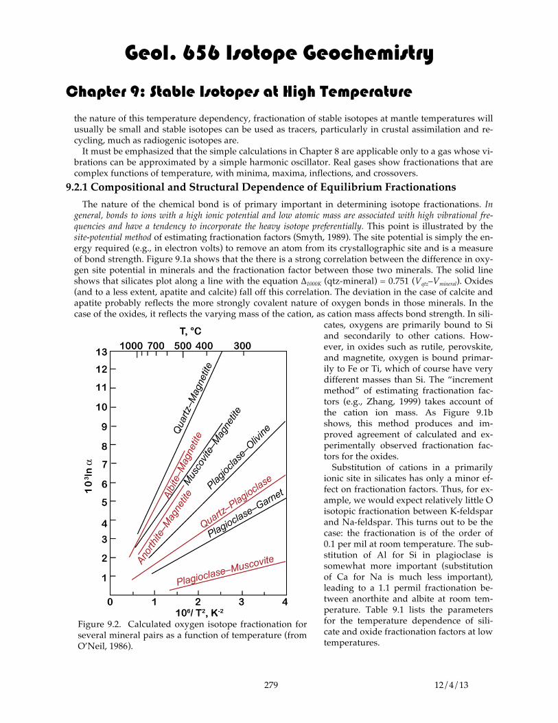
Figure 9.2. Calculated oxygen isotope fractionation for several mineral pairs as a function of temperature (from O’Neil, 1986).

Geol. 656 Isotope Geochemistry
Chapter 9: Stable Isotopes at High Temperature
280 12/4/13
Because oxygen occupies a generally similar lattice site in virtually all mantle and igneous minerals (it is covalently bonded to silicon and ionicly bonded to other cations such as Mg, Fe, Ca, etc.), frac-tionation of oxygen isotopes between these phases and during melting and crystallization are relatively small, although still measurable. Carbonates tend to be very 18O rich because O is bonded to a small, highly charged atom, C4+. The fractionation relative to water, ∆18O is about +30 for calcite. The cation (i.e., Ca or Mg in carbonate) has a secondary role (because of the effects of its mass on vibrational frequency). ∆18O decreases to about 25 for Ba (about 3 times the mass of Ca). Crystal structure usually plays a secondary role. The ∆18O between aragonite and calcite is of the or-der of 0.5 permil. But there apparently is a large fractionation (10 permil) of C between graphite and diamond extrapolated to room temperature. Pressure effects turn out to be small, 0.1 permil at 2 GPa and less. The reason should be fairly obvi-ous: there is no volume change is isotope exchange reactions, and pressure effects depend on volume changes. The volume of an atom is entirely determined by its electronic structure, which does not depend on the mass of the nucleus. On the other hand, there will be some minor fractionation that results from changes in vibrational frequency as crystals are compressed.
9.2.2 Geothermometry One of the principal uses of stable iso-topes is as geothermometers. Like conven-tional chemical geothermometers, stable isotope geothermometers are based on the temperature dependence of the equi-librium constant (equation 9.1). In actual-ity, the constants A and B in equation 9.1 are slowly varying functions of tem-perature, such that K tends to zero at abso-lute 0, corresponding to complete separa-tion, and to 1 at infinite temperature, corre-sponding to no isotope separation. We can obtain a qualitative understanding of why this is so by recalling that the entropy of a system increases with temperature. At infi-nite temperature, there is complete dis-order, hence isotopes would be mixed ran-domly between phases (ignoring for the moment the slight problem that at infinite temperature there would be neither phases nor nuclei). At absolute 0, there is perfect order, hence no mixing of isotopes between phases. A and B are, however, sufficiently invariant over a range of geologically in-teresting temperatures that as a practical matter they can be described as constants. We have also noted that at temperatures
Table 9.01. Coefficients Oxygen Isotope Frac-tionation at Low Temperatures:
ΔQZ-φ = A + B × 106/T2 φ Α Β Feldspar 0 0.97 + 1.04b* Pyroxene 0 2.75 Garnet 0 2.88 Olivine 0 3.91 Muscovite –0.60 2.2 Amphibole –0.30 3.15 Biotite –0.60 3.69 Chlorite –1.63 5.44 Ilmenite 0 5.29 Magnetite 0 5.27 * b is the mole fraction of anorthite in the feldspar. This term therefore accounts for the compositional dependence discussed above. From Javoy (1976). Table 9.2. Coefficients for Oxygen Isotope Fractionations at Elevated Temperatures (600° – 1300°C)
Cc Ab An Di Fo Mt Qz 0.38 0.94 1.99 2.75 3.67 6.29 Cc 0.56 1.61 2.37 3.29 5.91 Ab 1.05 1.81 2.73 5.35 An 0.76 1.68 4.30 Di 0.92 3.54 Fo 2.62 Coefficients are for mineral pair fractionations expressed as: 1000α = B×106/T2 where B is given in the Table. Qz: quartz, Cc: calcite, Ab: albite, An: anorthite, Di: diopside, Fo: forsterite, Mt: magnetite. For example, the fractionation between albite and diopside is 1000αΑλ−Δι = 1.81×10⁶/T2 (T in kelvins). From Chiba, et al. (1989).
Geol. 656 Isotope Geochemistry
Chapter 9: Stable Isotopes at High Temperature
281 12/4/13
close to room temperature and below, the form of equation 9.01 changes to K ∝ 1/T. Because of the dependence of the equilibrium constant on the inverse square of temperature, stable isotope geothermometry is employed primarily at low and moderate temperatures, that is, non-mag-matic temperatures. At temperatures greater than 800°C or so (there is no exact cutoff), the fractiona-tions are often too small for accurate temperatures to be calculated from them. In principal, a temperature may be calculated from the isotopic fractionation between any phases provided the phases achieved equilibrium and the temperature dependence of the fractionation factor is known. Indeed, there are too many isotope geothermometers for all of them to be even mentioned here. We can begin by considering silicate systems. Figure 9.2 shows fractionation factors between vari-ous silicates and oxides as a function of temperature. Tables 9.1 and 9.2 list coefficients A and B for tem-perature dependence of the fractionation factor between quartz and other common silicates and oxides when this temperature dependence is expressed as:
�
Δ ≅1000 lnαQz−φ = A+ BT 2 ×10
6 9.02
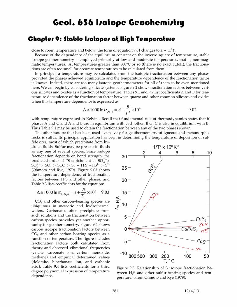
with temperature expressed in Kelvins. Recall that fundamental rule of thermodynamics states that if phases A and C and A and B are in equilibrium with each other, then C is also in equilibrium with B. Thus Table 9.1 may be used to obtain the fractionation between any of the two phases shown. The other isotope that has been used extensively for geothermometry of igneous and metamorphic rocks is sulfur. Its principal application has been in determining the temperature of deposition of sul-fide ores, most of which precipitate from hy-drous fluids. Sulfur may be present in fluids as any one of several species. Since isotope fractionation depends on bond strength, the predicted order of 34S enrichment is: SO4
2 −> SO 3
2 −> SO2 > SCO > Sx ~ H2S ~HS1– > S2–
(Ohmoto and Rye, 1979). Figure 9.03 shows the temperature dependence of fractionation factors between H2S and other phases, and Table 9.3 lists coefficients for the equation:
�
Δ ≅1000 lnαφ−H2S= A+ B
T 2 ×10⁶ 9.03
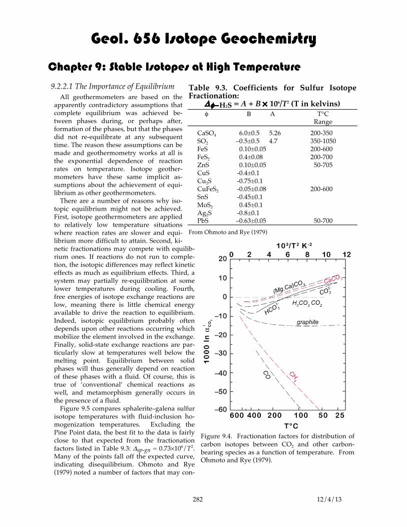
CO2 and other carbon–bearing species are ubiquitous in meteoric and hydrothermal waters. Carbonates often precipitate from such solutions and the fractionation between carbon-species provides yet another oppor-tunity for geothermometry. Figure 9.4 shows carbon isotope fractionation factors between CO2 and other carbon bearing species as a function of temperature. The figure includes fractionation factors both calculated from theory and observed vibrational frequencies (calcite, carbonate ion, carbon monoxide, methane) and empirical determined values (dolomite, bicarbonate ion, and carbonic acid). Table 9.4 lists coefficients for a third degree polynomial expression of temperature dependence.
Figure 9.3. Relationship of S isotope fractionation be-tween H2S and other sulfur-bearing species and tem-perature. From Ohmoto and Rye (1979).
Geol. 656 Isotope Geochemistry
Chapter 9: Stable Isotopes at High Temperature
282 12/4/13
9.2.2.1 The Importance of Equilibrium All geothermometers are based on the apparently contradictory assumptions that complete equilibrium was achieved be-tween phases during, or perhaps after, formation of the phases, but that the phases did not re-equilibrate at any subsequent time. The reason these assumptions can be made and geothermometry works at all is the exponential dependence of reaction rates on temperature. Isotope geother-mometers have these same implicit as-sumptions about the achievement of equi-librium as other geothermometers. There are a number of reasons why iso-topic equilibrium might not be achieved. First, isotope geothermometers are applied to relatively low temperature situations where reaction rates are slower and equi-librium more difficult to attain. Second, ki-netic fractionations may compete with equilib-rium ones. If reactions do not run to comple-tion, the isotopic differences may reflect kinetic effects as much as equilibrium effects. Third, a system may partially re-equilibration at some lower temperatures during cooling. Fourth, free energies of isotope exchange reactions are low, meaning there is little chemical energy available to drive the reaction to equilibrium. Indeed, isotopic equilibrium probably often depends upon other reactions occurring which mobilize the element involved in the exchange. Finally, solid-state exchange reactions are par-ticularly slow at temperatures well below the melting point. Equilibrium between solid phases will thus generally depend on reaction of these phases with a fluid. Of course, this is true of ‘conventional’ chemical reactions as well, and metamorphism generally occurs in the presence of a fluid. Figure 9.5 compares sphalerite–galena sulfur isotope temperatures with fluid-inclusion ho-mogenization temperatures. Excluding the Pine Point data, the best fit to the data is fairly close to that expected from the fractionation factors listed in Table 9.3: Δsp-gn = 0.73×10⁶/T2. Many of the points fall off the expected curve, indicating disequilibrium. Ohmoto and Rye (1979) noted a number of factors that may con-
Table 9.3. Coefficients for Sulfur Isotope Fractionation:
Δφ−H2S = A + B × 106/T2 (T in kelvins) φ Β A T°C Range CaSO4 6.0±0.5 5.26 200-350 SO2 –0.5±0.5 4.7 350-1050 FeS 0.10±0.05 200-600 FeS2 0.4±0.08 200-700 ZnS 0.10±0.05 50-705 CuS -0.4±0.1 Cu2S -0.75±0.1 CuFeS2 -0.05±0.08 200-600 SnS -0.45±0.1 MoS2 0.45±0.1 Ag2S -0.8±0.1 PbS –0.63±0.05 50-700 From Ohmoto and Rye (1979)
Figure 9.4. Fractionation factors for distribution of carbon isotopes between CO2 and other carbon-bearing species as a function of temperature. From Ohmoto and Rye (1979).

Geol. 656 Isotope Geochemistry
Chapter 9: Stable Isotopes at High Temperature
283 12/4/13
tribute to the lack of fit, such as impure mineral separates used in the analysis; for example, 10% of the galena in sphalerite and visa versa would result in an estimated temperature of 215°C if the actual equilibration temperature was 145°C. Different minerals may crystallize at different times and differ-ent temperatures in a hydrothermal system and hence would never be in equilibrium. In general, those minerals in direct contact with each other give the most reliable temperatures. Real disequilibrium may also occur if crys-tallization is kinetically controlled. The generally good fit to the higher temperature sulfides and poor fit to the low temperature ones sug-gests the temperature dependence of reaction kinetics may be the most important factor. Isotope geothermometers do have several advantages over con-ventional chemical ones. First, as we have noted, there is no volume change associated with isotopic ex-change reactions and hence little pressure dependence of the equi-librium constant (however, Rumble has suggested an indirect pressure dependence, wherein the fractiona-tion factor depends on fluid com-position which in turn depends on pressure). Second, whereas con-ventional chemical geothermome-ters are generally based on solid solution, isotope geothermometers can make use of pure phases such as SiO2, etc. Generally, any depen-dence on the composition of phases in isotope geothermometers in-volved is of relatively second order importance. For example, isotopic exchange between calcite and water is independent of the concen-tration of CO2 in the water. Compositional effects can be expected only where composition affects bonds formed by the element involved in the exchange. For example, we noted substitution of Al for Si in plagioclase affects O isotope fractionation factors because the nature of the bond with oxygen. The composition of a CO2 bearing solution, however, should not affect isotopic fractionation between calcite and dissolved carbonate because the oxygen is bonded with C regardless of the presence of other ions
Table 9.4 Isotope Fractionation Factors of Carbon Compounds with Respect to CO2 1000 Ln α = A × 108/T3 + B × 106/T2 + C × 103/T + D φ Α B C D T°C Range CaMg(CO3)2 -8.914 8.737 -18.11 8.44 ≤600 Ca(CO3) -8.914 8.557 -18.11 8.24 ≤600 HCO1–
3 0 -2.160 20.16 -35.7 ≤290 CO2–
3 -8.361 -8.196 -17.66 6.14 ≤100 H2CO3 0 0 0 0 ≤350 CH4 4.194 -5.210 -8.93 4.36 ≤700 CO 0 -2.84 -17.56 9.1 ≤330 C -6.637 6.921 -22.89 9.32 ≤700 From Ohmoto and Rye (1979).
Figure 9.05. Comparison of temperatures determined from sphalerite–galena sulfur isotope fractionation with fluid-in-clusion homogenization temperatures. J: Creede, CO, S: Sun-nyside, O: Finlandia vein, C: Pasto Bueno, G: Kuroko. From Ohmoto and Rye (1979).

Geol. 656 Isotope Geochemistry
Chapter 9: Stable Isotopes at High Temperature
284 12/4/13
(if we define the fractionation as between water and calcite, some effect is possible if the O in the car-bonate radical exchanges with other radicals present in the solution).
9.3 STABLE ISOTOPE COMPOSITION OF THE MANTLE Before we can use stable isotope ratios as indicators of crustal assimilation and tracers of crustal recy-cling, we need to define the stable isotopic composition of “uncontaminated” mantle. It is, however, important to recognize from the outset that, in a strict sense, there may be no such thing. We found in our consideration of radiogenic isotope ratios that no samples of “primitive” mantle have been recov-ered: the mantle, or at least that portion sampled by volcanism, has been pervasively processed. A very considerable amount of oceanic crust has been subducted during this time, perhaps accompanied by sediment. As we shall see, the stable isotopic composition of the oceanic crust is extensively modified by hydrothermal processes and low temperature weathering. Subduction of this material has the potential for modifying the stable isotopic composi-tion of the mantle. Thus while we will attempt to use stable isotope ratios to identify “contamination” of mantle by subduction, we must recognize all of it may have been “contaminated” to some degree. Other problems arise in defining the stable isotope composition of the man-tle. We relied heavily on basalts as mantle samples in defining the radio-genic isotope composition of the man-tle. We could do so because radiogenic isotope ratios are not changed in the magma generation process. This will not be strictly true of stable isotope ra-tios, which can be changed by chemical processes. The effects of the melting process on most stable isotope ratios of interest are small, but not completely negligible. Degassing does significantly affect stable isotope ratios, particularly those of carbon and hydrogen, which compromises the value of magmas as a mantle sample. Once oxides begin to crystallize, fractional crystallization will affect oxygen isotope ratios, al-though the resulting changes are, as we shall see, only a few per mil even in ex-treme cases. Finally, weathering and hydrothermal processes can affect sta-ble isotope ratios of basalts and other igneous rocks. Because hydrogen, car-bon, nitrogen, and sulfur are all trace elements in basalts but are quite abun-
Figure 9.6. Oxygen isotope ratios in olivines and cli-nopyroxenes from mantle peridotite xenoliths. From Mat-tey et al. (1994).
Geol. 656 Isotope Geochemistry
Chapter 9: Stable Isotopes at High Temperature
285 12/4/13
dant at the Earth’s surface, these elements are particularly sus-ceptible to weathering effects. Even oxygen, which constitutes nearly 50% by weight of silicate rocks, is readily affected by weathering. Thus we will have to proceed with some caution in using basalts as samples of the mantle for stable isotope ra-tios.
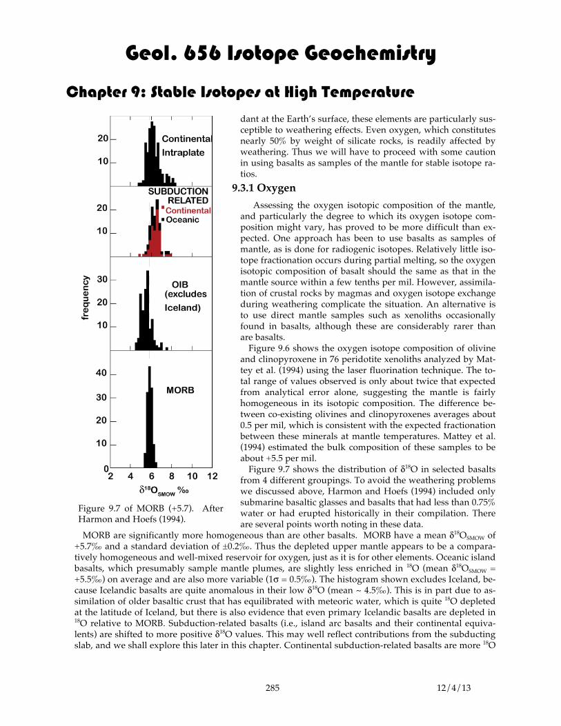
9.3.1 Oxygen Assessing the oxygen isotopic composition of the mantle, and particularly the degree to which its oxygen isotope com-position might vary, has proved to be more difficult than ex-pected. One approach has been to use basalts as samples of mantle, as is done for radiogenic isotopes. Relatively little iso-tope fractionation occurs during partial melting, so the oxygen isotopic composition of basalt should the same as that in the mantle source within a few tenths per mil. However, assimila-tion of crustal rocks by magmas and oxygen isotope exchange during weathering complicate the situation. An alternative is to use direct mantle samples such as xenoliths occasionally found in basalts, although these are considerably rarer than are basalts. Figure 9.6 shows the oxygen isotope composition of olivine and clinopyroxene in 76 peridotite xenoliths analyzed by Mat-tey et al. (1994) using the laser fluorination technique. The to-tal range of values observed is only about twice that expected from analytical error alone, suggesting the mantle is fairly homogeneous in its isotopic composition. The difference be-tween co-existing olivines and clinopyroxenes averages about 0.5 per mil, which is consistent with the expected fractionation between these minerals at mantle temperatures. Mattey et al. (1994) estimated the bulk composition of these samples to be about +5.5 per mil. Figure 9.7 shows the distribution of δ18O in selected basalts from 4 different groupings. To avoid the weathering problems we discussed above, Harmon and Hoefs (1994) included only submarine basaltic glasses and basalts that had less than 0.75% water or had erupted historically in their compilation. There are several points worth noting in these data.
MORB are significantly more homogeneous than are other basalts. MORB have a mean δ18OSMOW of +5.7‰ and a standard deviation of ±0.2‰. Thus the depleted upper mantle appears to be a compara-tively homogeneous and well-mixed reservoir for oxygen, just as it is for other elements. Oceanic island basalts, which presumably sample mantle plumes, are slightly less enriched in 18O (mean δ18OSMOW = +5.5‰) on average and are also more variable (1σ = 0.5‰). The histogram shown excludes Iceland, be-cause Icelandic basalts are quite anomalous in their low δ18O (mean ~ 4.5‰). This is in part due to as-similation of older basaltic crust that has equilibrated with meteoric water, which is quite 18O depleted at the latitude of Iceland, but there is also evidence that even primary Icelandic basalts are depleted in 18O relative to MORB. Subduction-related basalts (i.e., island arc basalts and their continental equiva-lents) are shifted to more positive δ18O values. This may well reflect contributions from the subducting slab, and we shall explore this later in this chapter. Continental subduction-related basalts are more 18O
Figure 9.7 of MORB (+5.7). After Harmon and Hoefs (1994).

Geol. 656 Isotope Geochemistry
Chapter 9: Stable Isotopes at High Temperature
286 12/4/13
rich than their oceanic equivalents, most likely due to assimilation of continental crust. Finally, con-tinental intraplate volcanics are more enriched in 18O than are OIB, again suggestive of crustal assimila-tion.
9.3.2 Carbon The stable isotopes of H, C, N, and S are much more difficult to analyze in igneous rocks. These ele-ments are generally trace elements and are volatile. With rare exceptions, they have a strong tendency to exsolve from the melt and escape as gases as magmas approach the surface of the Earth. Not only are these elements lost during degassing but they also can be isotopically fractionated in the process. Thus there is far less data on the isotopes of these elements in basalts, and the meaning of this data is some-what open to interpretation. Most carbon in basalts is in the form of CO2, which has limited solubility in basaltic liquids at low pressure. As a result, basalts begin to exsolve CO2 before they erupt. Thus virtually every basalt sample has lost some carbon, and subareal basalts have lost virtually all carbon (as well as most other vola-tiles). Therefore, only basalts erupted beneath several km of water provide useful samples of mantle carbon. As a result, the data set is restricted to MORB, samples recovered from Loihi and the submarine part of Kilauea’s East Rift Zone, and a few other seamounts. The question of the isotopic composition of mantle carbon is further complicated by fractionation and contamination. There is a roughly 4‰ fractionation between CO2 dissolved in basaltic melts and the gas phase, with 13C enriched in the gas phase. If Rayleigh distillation occurs, that is if bubbles do not
remain in equilibrium with the liquid, then the basalt that eventually erupts may have carbon that is substantially lighter than the carbon originally dissolved in the melt. Furthermore, MORB are pervasively contaminated with a very 13C-depleted carbon. This carbon is proba-bly organic in origin, and recent observations of an eruption on the East Pacific Rise suggest a source. Following the 1991 eruption at 9°30’ N, there was an enormous ‘bloom’ of bacteria stimulated by the release of H2S. Bacterial mats covered everything. The remains of these bac-teria may be the source of this organic carbon. Fortunately, it appears possible to avoid most of this contamination by the step-wise heating procedure now used by most laboratories. Most of the contaminant carbon is released at temperatures below 600°C, whereas most of the basaltic carbon is released above 900°C. Figure 9.8 shows δ13C in various mantle and mantle-derived materials. MORB have a mean δ13C of -6.5 and a standard deviation of 1.7. Hawaiian basalts appear to have slightly heav-ier carbon. Xenoliths in oceanic island basalts are also slightly heavier than MORB. Whether this reflects a real difference in isotopic compo-sition or merely the effect of fractionation is unclear. The most CO2-rich MORB samples have δ13C of about –4. Since they are the least
Figure 9.8. Carbon isotope ratios in mantle (red) and mantle-derived materials (gray). After Mattey (1987).

Geol. 656 Isotope Geochemistry
Chapter 9: Stable Isotopes at High Temperature
287 12/4/13
degassed, they presumably best represent the isotopic composition of the depleted mantle (Javoy and Pineau, 1991). If this is so, there may be little difference in carbon isotopic composition between MORB and oceanic islands sampled thus far (which include only Hawaii, Reunion, and Kerguelen). Gases re-leased in subduction zone volcanoes have δ13C that ranges from 0 to –10‰, with most values being in the range of –2 to –4‰, comparable to the most gas-rich MORB (Javoy, et al., 1986). Continental xeno-liths are more heterogeneous in carbon isotopic composition than other groups, and the meaning of this is unclear. Carbonatites have somewhat lighter carbon than most MORB. Diamonds show a large range of carbon isotopic compositions (Figure 9.8). Most diamonds have δ13C within the range of -2 to -8‰, hence similar to MORB. However, some diamonds have much lighter carbon. Based on the inclusions they contain, diamonds can be divided between peridotitic and ec-logitic. Most peridotitic diamonds have δ13C close to –5‰, while eclogitic diamonds are much more iso-topically variable. Most, though not all, of the diamonds with very negative δ13C are eclogitic. Many diamonds are isotopically zoned, indicating they grew in several stages. Three hypotheses have been put forward to explain the isotopic heterogeneity in diamonds: pri-mordial heterogeneity, fractionation effects, and recycling of organic carbon from the Earth’s surface into the mantle. Primordial heterogeneity seems unlikely for a number of reasons. Among these are the absence of very negative δ13C in other materials, such as MORB, and the absence of any evidence for primordial heterogeneity from the isotopic compositions of other elements. Boyd and Pillinger (1994) have argued that since diamonds are kinetically sluggish (witness their stability at the surface of the Earth, where they are thermodynamically out of equilibrium), isotopic equilibrium might not achieved during their growth. Large fractionations might therefore occur due to kinetic effects. However, these kinetic fractionations have not been demonstrated, and fractionations of this magnitude (20‰ or so) would be surprising at mantle temperatures. On the other hand, several lines of evidence support the idea that isotopically light carbon in some diamonds had its origin as organic carbon at the Earth’s surface. First, such diamonds are primarily of eclogitic paragenesis and eclogite is the high pressure equivalent of basalt. Subduction of oceanic crust continuously carries large amounts of basalt into the mantle. Oxygen isotope heterogeneity observed in some eclogite xenoliths suggests these eclogites do indeed represent subducted oceanic crust. Second,
the nitrogen isotopic composition of isotopi-cally light diamonds are anomalous relative to nitrogen in other mantle materials yet similar to nitrogen in sedimentary rocks.
9.3.3 Hydrogen Like carbon, hydrogen can be lost from ba-salts during degassing. On the one hand, the problem is somewhat less severe than for carbon because the solubility of water in ba-salt is much greater than that of CO2. Basalts erupted beneath a kilometer of more of water probably retain most of their dissolved water. However, basalts, particularly submarine ba-salts, are far more readily contaminated with hydrogen (i.e., with water) than with carbon. Furthermore, the effect on hydrogen isotopic composition depends on the mode of con-tamination, as Figure 9.9 indicates. Direct ad-dition of water or hydrothermal reactions will raise δD (because there is little fractiona-
Figure 9.9. Effect of degassing and post-eruptive processes on the water content and δD of basalts. From Kyser and O’Neil (1984).
Geol. 656 Isotope Geochemistry
Chapter 9: Stable Isotopes at High Temperature
288 12/4/13
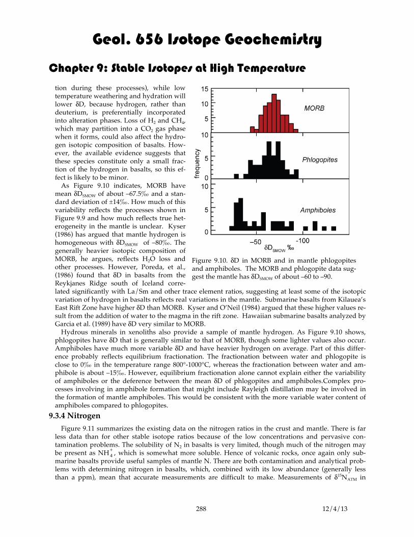
tion during these processes), while low temperature weathering and hydration will lower δD, because hydrogen, rather than deuterium, is preferentially incorporated into alteration phases. Loss of H2 and CH4, which may partition into a CO2 gas phase when it forms, could also affect the hydro-gen isotopic composition of basalts. How-ever, the available evidence suggests that these species constitute only a small frac-tion of the hydrogen in basalts, so this ef-fect is likely to be minor. As Figure 9.10 indicates, MORB have mean δDSMOW of about –67.5‰ and a stan-dard deviation of ±14‰. How much of this variability reflects the processes shown in Figure 9.9 and how much reflects true het-erogeneity in the mantle is unclear. Kyser (1986) has argued that mantle hydrogen is homogeneous with δDSMOW of –80‰. The generally heavier isotopic composition of MORB, he argues, reflects H2O loss and other processes. However, Poreda, et al., (1986) found that δD in basalts from the Reykjanes Ridge south of Iceland corre-lated significantly with La/Sm and other trace element ratios, suggesting at least some of the isotopic variation of hydrogen in basalts reflects real variations in the mantle. Submarine basalts from Kilauea’s East Rift Zone have higher δD than MORB. Kyser and O’Neil (1984) argued that these higher values re-sult from the addition of water to the magma in the rift zone. Hawaiian submarine basalts analyzed by Garcia et al. (1989) have δD very similar to MORB. Hydrous minerals in xenoliths also provide a sample of mantle hydrogen. As Figure 9.10 shows, phlogopites have δD that is generally similar to that of MORB, though some lighter values also occur. Amphiboles have much more variable δD and have heavier hydrogen on average. Part of this differ-ence probably reflects equilibrium fractionation. The fractionation between water and phlogopite is close to 0‰ in the temperature range 800°-1000°C, whereas the fractionation between water and am-phibole is about –15‰. However, equilibrium fractionation alone cannot explain either the variability of amphiboles or the deference between the mean δD of phlogopites and amphiboles.Complex pro-cesses involving in amphibole formation that might include Rayleigh distillation may be involved in the formation of mantle amphiboles. This would be consistent with the more variable water content of amphiboles compared to phlogopites.
9.3.4 Nitrogen Figure 9.11 summarizes the existing data on the nitrogen ratios in the crust and mantle. There is far less data than for other stable isotope ratios because of the low concentrations and pervasive con-tamination problems. The solubility of N2 in basalts is very limited, though much of the nitrogen may be present as NH 4
+ , which is somewhat more soluble. Hence of volcanic rocks, once again only sub-marine basalts provide useful samples of mantle N. There are both contamination and analytical prob-lems with determining nitrogen in basalts, which, combined with its low abundance (generally less than a ppm), mean that accurate measurements are difficult to make. Measurements of δ15NATM in
Figure 9.10. δD in MORB and in mantle phlogopites and amphiboles. The MORB and phlogopite data sug-gest the mantle has δDSMOW of about –60 to –90.

Geol. 656 Isotope Geochemistry
Chapter 9: Stable Isotopes at High Temperature
289 12/4/13
MORB range from about –2 to +12‰. The few available analyses of Hawaiian basalts range up to +20. At present, it is very difficult to decide to what degree this variation reflects contamination (par-ticularly by organic matter), fractionation during degassing, or real mantle hetero-geneity. Perhaps all that can be said is that nitrogen in basalts appears to have positive δ15N on average. Diamonds can contain up to 2000 ppm of N and hence provide an excellent sample of mantle N. As can be seen in Figure 9.11, high δ13C diamonds (the ones most common and usually of peridotitic paragenesis) have δ15N that range from -12 to +5 and average about -3‰, which contrasts with the generally positive val-ues observed in basalts. Low δ13C dia-monds have generally positive δ15N. Since organic matter and ammonia in crustal rocks generally have positive δ15N, this characteristic is consistent with the hypothesis that this group of dia-monds are derived from subducted crustal material. However, since basalts appear to have generally positive δ15N, other interpretations are also possible. Fibrous diamonds, whose growth may be directly related to the kimberlite eruptions that carry them to the surface (Boyd et al., 1994), have more uniform δ15N, with a mean of about -5‰. Since there can be significant isotopic fractionations involved in the incorporation of nitrogen into diamond, the meaning of the diamond data is also uncertain, and the question of the nitrogen isotopic composition of the man-tle remains an open one.
9.3.5 Sulfur There are also relatively few sulfur isotope measurements on basalts, in part because sulfur is lost during degassing, except for those basalts erupted deeper than 1 km below sealevel. In the mantle, sul-fur is probably predominantly or exclusively in the form of sulfide, but in basalts, which tend to be somewhat more oxidized, some of it may be present as SO2 or sulfate. Equilibrium fractionation should lead to SO2 being a few per mil lighter than sulfate. If H2S is lost during degassing the remaining sulfur would become heavier; if SO2 or SO 4
2 − is lost, the remaining sulfur would become lighter. Total sulfur in MORB has δ34SCDT in the range of +1.3 to –1‰, with most values in the range 0 to +1‰. Sakai et al. (1984) found that sulfate in MORB, which constitutes 10-20% of total sulfur, was 3.5 to 9‰ heavier than sulfide. Basalts from Kilauea’s East Rift Zone have a very restricted range of δ34S of +0.5 to +0.8 (Sakai, et al., 1984). Chaussidon et al. (1989) analyzed sulfides present as inclusions in minerals, both in basalts and in xenoliths, and found a wide range of δ34S (–5 to +8‰). Low Ni sulfides in oceanic island basalts, kim-berlites, and pyroxenites had more variable δ34S than sulfides in peridotites and peridotite minerals. They argued there is a fractionation of +3‰ between sulfide liquid and sulfide dissolved in silicate
Figure 9.11. Isotopic composition of nitrogen in rocks and minerals of the crust and mantle. Modified from Boyd and Pillinger (1994).

Geol. 656 Isotope Geochemistry
Chapter 9: Stable Isotopes at High Temperature
290 12/4/13
melt. Carbonatites have δ34S between +1 and –3‰ (Hoefs, 1986; Kyser, 1986). Overall, it appears the mantle has a mean δ34S in the range of 0 to +1‰, which is very similar to meteorites, which average about +0.1‰. Chaussidon, et al. (1987) found that sulfide inclusions in diamonds of peridotitic paragenesis (δ13C ~ -4‰) had δ34S of about +1‰ while eclogitic diamonds had higher, and much more variable δ34S (+2 to +10‰). Eldridge et al. (1991) found that δ34S in diamond inclusions was related to the Ni content of the sulfide. High Ni sulfide inclusions, which they argued were of peridotitic paragenesis, had δ34S be-tween +4‰ and –4‰. Low Ni sulfides, which are presumably of eclogitic paragenesis, had much more variable δ34S (+14‰ to –10). These results are consistent with the idea that eclogitic diamonds are de-rived from subducted crustal material.
9.4 OXYGEN ISOTOPES IN MAGMATIC PROCESSES As we found earlier, the equilibrium constant of isotope exchange reactions, K, is proportional to the inverse square temperature and consequently isotopic fractionation at high temperature is small. In magmatic systems, another factor limiting the fractionation of stable isotopes is the limited variety of bonds that O is likely to form. Most of the oxygen in silicates and in silicate liquids is not present as free ions, but is bound to silicon atoms to form silica tetrahedra, which will be linked to varying degrees depending on the composition of the mineral or the composition of the melt. The silica tetrahedra and the Si–O bonds in a silicate melt are essentially identical to those in silicate minerals. Thus we would expect the fractionation of oxygen isotopes between silicate liquids (magmas) and silicate minerals crys-tallizing from those liquids to be rather limited. We would expect somewhat greater fractionation when non-silicates such as magnetite (Fe3O4) crystallize. In general, crystallization of quartz will lead to a de-pletion of 18O in the melt, crystallization of silicates such as olivine, pyroxene, hornblende, and biotite will lead to slight enrichment of the melt in 18O, and crystallization of oxides such as magnetite and il-menite will lead to a more pronounced enrichment of the melt in 18O (however, oxides such as magnet-ite are generally only present at the level of a few percent in igneous rocks, which limits their effect). Crystallization of feldspars can lead to either enrichment or depletion of 18O, depending on the tem-perature and the composition of the feldspar and the melt. Because quartz generally only crystallizes
very late, the general effect of fractional crystallization on magma is generally to increase δ18O slightly, generally not more than a few per mil. On the other hand, water-rock in-teraction at low to moderate temperatures at the surface of the Earth, produces much larger O isotopic changes, gen-erally enriching the rock in 18O. Consequently, crustal rocks show significant variability in δ18O. As we have seen, the range of δ18OSMOW in the fresh, young basalts and other mantle mate-rials is about +4.5 to +7. Be-cause this range is narrow, and the range of those crustal mate-rials is much greater, O isotope
Figure 9.12. Plot of δ18O versus fraction of magma solidified dur-ing Rayleigh fractionation, assuming the original δ18O of the magma was +6. After Taylor and Sheppard (1986).

Geol. 656 Isotope Geochemistry
Chapter 9: Stable Isotopes at High Temperature
291 12/4/13
ratios are a sensitive indicator of crustal assimilation. Isotope ratios outside this range suggest, but do not necessarily prove, the magmas have assimilated crust (or that post-eruptional isotopic exchange has occurred).
9.4.1 Oxygen Isotope Changes during Crystallization The variation in O isotope composition produced by crystallization of magma will depend on the manner in which crystallization proceeds. The simplest, and most unlikely, case is equilibrium crys-tallization. In this situation, the crystallizing minerals remain in isotopic equilibrium with the melt until crystallization is complete. At any stage during crystallization, the isotopic composition of a mineral and the melt will be related by the fractionation factor, α. Upon complete crystallization, the rock will have precisely the same isotopic composition as the melt initially had. At any time during the crystalli-zation, the isotope ratio in the remaining melt will be related to the original isotope ratio as:
RR0
=1
f +α(1− f ) ; α =
Rs
R 9.4
where Rl is the ratio in the liquid, Rs is the isotope ratio of the solid, R0 is the isotope ratio of the original magma, ƒ is the fraction of melt remaining. This equation is readily derived from mass balance, the definition of α, and the assumption that the O concentration in the magma is equal to that in the crys-tals; an assumption valid to about 10%. Since we generally do not work with absolute ratios of stable isotopes, it is more convenient to express 9.04, in terms of δ:
Δ = δmelt − δ0 ≅1
ƒ +α(1− ƒ)−1⎡
⎣⎢⎤⎦⎥×1000 9.5
where δmelt is the value of the magma after a fraction ƒ-1 has crystallized and δo is the value of the origi-nal magma. For silicates, α is not likely to be much less than 0.998 (i.e., ∆ = δ18Omelt – δ18Oxtals ≤ 2). For α = 0.999, even after 99% crystallization, the isotope ratio in the remaining melt will change by only 1 per mil. Fractional crystallization is a process analogous to Rayleigh distillation. Indeed, it is governed by the same equation (8.80), which we can rewrite as:
Δ = 1000( f α−1 −1) 9.6 The key to the operation of either of these processes is that the product of the reaction (vapor in the case of distillation, crystals in the case of crystallization) is only instantane-ously in equilibrium with the origi-nal phase. Once it is produced, it is removed from further opportunity to equilibrate with the original phase. This process is more efficient at pro-ducing isotopic variations in igneous rocks, but its effect remains limited because α is generally not greatly dif-ferent from 1. Figure 9.12 shows cal-culated changes in the isotopic com-position of melt undergoing frac-tional crystallization for various val-
Figure 9.13. δ18O as a function of SiO2 in a tholeiitic suite from the Galapagos Spreading Center (GSC) (Muehlenbachs and Byerly, 1982) and an alkaline suite from Ascension Island (Sheppard and Harris, 1985). Dashed line shows model calcu-lation for the Ascension suite.

Geol. 656 Isotope Geochemistry
Chapter 9: Stable Isotopes at High Temperature
292 12/4/13
ues of ∆ (≈ 1000(α–1)). In reality, ∆ will change during crystallization because of (1) changes in tem-perature (2) changes in the minerals crystallizing, and (3) changes in the liquid composition. The changes will generally mean that the effective ∆ will increase as crystallization proceeds. We would ex-pect the greatest isotopic fractionation in melts crystallizing non-silicates such as magnetite and melts crystallizing at low temperature, such as rhyolites, and the least fractionation for melts crystallizing at highest temperature, such as basalts. Figure 9.13 shows observed δ18O as a function of temperature in two suites: one from a propagating rift on the Galapagos Spreading Center (GSC), the other from the island of Ascension. There is a net change in δ18O between the most and least differentiated rocks in the GSC of about 1.3‰; the change in the Ascension suite is only about 0.5‰. These, and other suites, indicate the effective ∆ is generally small, on the order of 0.1 to 0.3‰. We can generalize the temperature dependence of stable isotopes by saying that at low temperature (ambient temperatures at the surface of the Earth up to the temperature of hydrothermal systems, 300-400° C), stable isotope ratios are changed by chemical processes. The amount of change can be used as an indication the nature of the process involved, and, under equilibrium conditions, of the temperature at which the process occurred. At high temperatures (temperatures of the interior of the Earth or mag-matic temperatures), chemical processes only minimally affect stable isotope ratios; they can therefore be used as tracers much as radiogenic isotope ratios are. These generalizations lead to a final axiom: igneous rocks whose oxygen isotopic compositions show signifi-cant variations from the primordial value (~6) must either have been affected by low temperature processes, or must contain a component that was at one time at the surface of the earth (Taylor and Sheppard, 1986). Rocks that have equilibrated with water at the surface of the Earth, e.g., sediments, tend to have δ18O values significantly higher than +6. Water on the surface of the Earth typically has δ18O significantly lower than +6 (0 for seawater, generally lower for meteoric water as we found in the last Chapter). In-terestingly, the δD values of sedimentary rocks and mantle-derived igneous rocks are rather similar (- 50 to -85). This may be coincidental since the δD of sediments are controlled by fractionation between minerals and water, whereas δD of igneous rocks reflects the isotopic composition of mantle hydrogen (mantle water). One the other hand, it is possible that it is not coincidental. Plate tectonics results in the return of water-being rocks from the surface of the Earth to the mantle (i.e., via subduction). It may well be that after 4.5 billion years, the subduction process essentially con-trols the isotopic composition of H in the upper mantle.
9.4.2 Combined Fractional Crystallization and Assimilation
Because oxygen isotope ratios of man-tle-derived magmas are uniform (with a few per mil) and generally different from rocks that have equilibrated with water at the surface of the Earth, oxygen iso-topes are a useful tool in identifying and studying the assimilation of country rock by intruding magma. We might think of this process as simple mixing between two components: magma and country
Figure 9.14. Variation in δ18O of a magma undergoing AFC vs. fraction crystallized computed using equation 9.07. Ini-tial δ18O of the magma is +6, δ18O of the assimilant is +18, ∆ = +1. R is the ratio of mass assimilated to mass crystallized.

Geol. 656 Isotope Geochemistry
Chapter 9: Stable Isotopes at High Temperature
293 12/4/13
rock. In reality, it is always at least a three-component problem, involving country rock, magma, and minerals crystallizing from the magma. Magmas are essentially never superheated; hence the heat re-quired to melt and assimilate surrounding rock can only come from the latent heat of crystallization of the magma. Approximately 1000 J/g would be required to heat rock from 150° C to 1150°C and another 300 J/g would be required to melt it. If the latent heat of crystallization is 400 J/g, crystallization of 3.25 g of magma would be required to assimilate 1 g of cold country rock. Since some heat will be lost by simple conduction to the surface, we can conclude that the amount of crystallization will inevitably be greater than the amount of assimilation (the limiting case where mass crystallized equals mass assimi-lated could occur only at very deep layers of the crust where the rock is at its melting point to begin with). The change in isotopic composition of a melt undergoing the combined process of assimilation and fractional crystallization (AFC) is given by:
δm −δ 0 = [δ a −δ 0 ]+∆R
⎛⎝⎜
⎞⎠⎟ 1− f −R/(R−1){ } 9.7
where R is the mass ratio of material assimilated to material crystallized, ∆ is the difference in isotope ratio between the crystals and the magma (δmagma-δcrystals), ƒ is the fraction of liquid remaining, δm is the δ18O of the magma, δo is the initial δ18O of the magma, and δa is the δ18O of the material being assimi-lated. (This equation is from DePaolo (1981) but differs slightly because we changed the definition of ∆.) The assumption is made that the concentration of oxygen is the same in the crystals, magma, and as-similant, which is a reasonable assumption. This equation breaks down at R = 1, but as discussed above, this is unlikely: R will always be less than 1. Figure 9.14 shows the variation of δ18O of a magma with an initial δ18O = 5.7 as crystallization and assimilation proceed.
9.4.3 Combining Radiogenic and Oxygen Isotopes A more powerful tool for the study of assimilation processes can result if O isotopes are combined with a radiogenic isotope ratio such as 87Sr/86Sr. There are several reasons for this. First, radiogenic iso-topes and stable isotopes each have their own ad-vantages. In the case of ba-saltic magmas, radiogenic elements, particularly Nd and Pb, often have lower concentrations in the magma than in the assimi-lant. This means a small amount of assimilant will have a large effect on the radiogenic isotope ratios. On the other hand, oxygen will be present in the magma and assimilant at nearly the same concentra-tion, making calculation of the mass assimilated fairly straightforward. Also, it is easier to uniquely charac-terize the assimilant using both radiogenic and stable isotope ratios, as suggested
Figure 9.15. δ18O vs. 87Sr/86Sr showing range of isotopic composition in various terrestrial rocks. After Taylor and Sheppard (1986).
Geol. 656 Isotope Geochemistry
Chapter 9: Stable Isotopes at High Temperature
294 12/4/13
in Figure 9.15. The equation governing a radiogenic isotope ratio in a magma during AFC is different from 9.7 be-cause we cannot assume the concentration of the element is the same in all the components. On the other hand, there is no fractionation between crystals and melt. The general equation describing the variation of the concentration of an element in a magma during AFC is:
Cm
Cm0 = f − z + R
R −1⎛⎝⎜
⎞⎠⎟Ca
Cm0 (1− f − z ) 9.8
where Cm and the concentration of the element in the magma, Co is the original magma concentration, ƒ is as defined for equation 9.7 above, and z is as:
z =R + D −1R −1
9.9
where D is the solid/liquid partition coefficient. The isotopic composition of the magma is the given by (DePaolo, 1981):
�
εm =
RR−1
⎛ ⎝ ⎜
⎞ ⎠ ⎟ Ca
z(1− f −z )εa +Cm
0 f −zε0
RR−1
⎛ ⎝ ⎜
⎞ ⎠ ⎟ Ca
z(1− f −z )+Cm
0 f −z 9.10
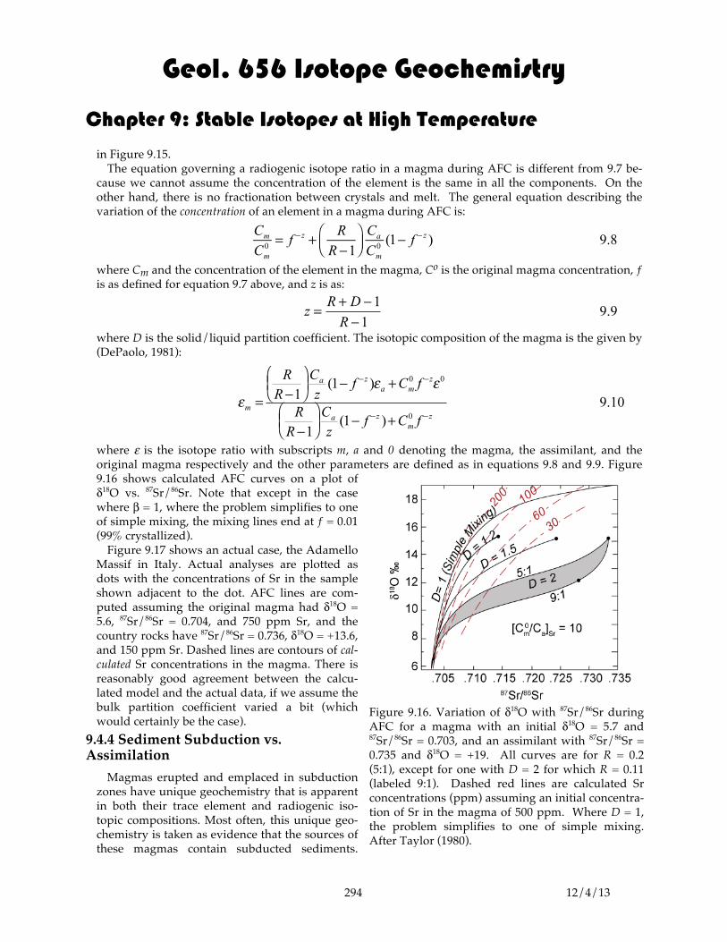
where ε is the isotope ratio with subscripts m, a and 0 denoting the magma, the assimilant, and the original magma respectively and the other parameters are defined as in equations 9.8 and 9.9. Figure 9.16 shows calculated AFC curves on a plot of δ18O vs. 87Sr/86Sr. Note that except in the case where β = 1, where the problem simplifies to one of simple mixing, the mixing lines end at ƒ = 0.01 (99% crystallized). Figure 9.17 shows an actual case, the Adamello Massif in Italy. Actual analyses are plotted as dots with the concentrations of Sr in the sample shown adjacent to the dot. AFC lines are com-puted assuming the original magma had δ18O = 5.6, 87Sr/86Sr = 0.704, and 750 ppm Sr, and the country rocks have 87Sr/86Sr = 0.736, δ18O = +13.6, and 150 ppm Sr. Dashed lines are contours of cal-culated Sr concentrations in the magma. There is reasonably good agreement between the calcu-lated model and the actual data, if we assume the bulk partition coefficient varied a bit (which would certainly be the case).
9.4.4 Sediment Subduction vs. Assimilation
Magmas erupted and emplaced in subduction zones have unique geochemistry that is apparent in both their trace element and radiogenic iso-topic compositions. Most often, this unique geo-chemistry is taken as evidence that the sources of these magmas contain subducted sediments.
Figure 9.16. Variation of δ18O with 87Sr/86Sr during AFC for a magma with an initial δ18O = 5.7 and 87Sr/86Sr = 0.703, and an assimilant with 87Sr/86Sr = 0.735 and δ18O = +19. All curves are for R = 0.2 (5:1), except for one with D = 2 for which R = 0.11 (labeled 9:1). Dashed red lines are calculated Sr concentrations (ppm) assuming an initial concentra-tion of Sr in the magma of 500 ppm. Where D = 1, the problem simplifies to one of simple mixing. After Taylor (1980).

Geol. 656 Isotope Geochemistry
Chapter 9: Stable Isotopes at High Temperature
295 12/4/13
However, in many instances, this interpreta-tion is non-unique. The geochemical signa-ture of subducted sediment is, in many re-spects, simply the signature of continental crust. In general, it is just as plausible that magmas have acquired this signature through assimilation of continental crust as by partial melting of a mantle containing subducted sediment. Magaritz et al. (1978) pointed out that by combining radiogenic isotope and oxygen isotope analyses, it is possible to distinguish between these two possibilities. Magaritz et al. reasoned as follows. First, many continental materials have oxygen iso-tope ratios that are quite different from man-tle values (e.g., Figure 9.18). Then they noted that all rocks have similar oxygen concentra-tions. Because of this, addition of 10% sedi-ment with δ18O of +20 to the mantle (+6) fol-lowed by melting of that mantle produces a magma with the same δ18O (+8.4), as adding 10% sediment directly to the magma (i.e., in this case the magma also ends up with δ18O = +8.4). However, addition of 10% sediment to the mantle, followed by melting of that mantle produces a magma with a very different Sr iso-tope ratio than does adding 10% sediment di-rectly to the magma. The reason for this differ-ence is that the Sr concentration of the magma is much higher (an order of magnitude or more higher) than that of the mantle. Thus addition of sediment to magma affects the Sr isotope ra-tio less than addition of sediment to the mantle. Indeed, most subduction-related magmas are richer in Sr (~ 400 ppm) than most continental materials and sediments; but sediments in-variably have more Sr than does the mantle (10-40 ppm). This point is illustrated in a more quantita-tive fashion in Figure 9.18. We discussed mix-ing trajectories earlier and noted that when two materials are mixed in varying proportions, a curve results on a plot of one ratio against an-other. The degree and sense of curvature depended on the ratio of the ratio of the two denominators in the two end-members. Since the concentration of oxygen is approximately the same in most rocks, the ratio of 16O in the two end-members can be taken as 1. So, for example, in plot of 87Sr/86Sr vs. oxygen isotope ratio, the degree of curvature depends only on the ratio of Sr in the two end-members. In Figure 9.18, when the ratio of Sr in end-member M (magma or mantle) to Sr in end-member C (crust or sed-
Figure 9.18. Mixing curves on a plot of δ18O vs. 87Sr/86Sr. The labels on the lines refer to different ratios of Sr concentration in the two end-members. After James (1981).
Figure 9.17. Variation of δ18O with 87Sr/86Sr in the Ada-mello Massif in Italy compared with model AFC process using equation 9.07- 9.10. After Taylor and Sheppard (1986).

Geol. 656 Isotope Geochemistry
Chapter 9: Stable Isotopes at High Temperature
296 12/4/13
iment) is greater than 1, a concave down-ward mixing curve results. If that ratio is less than 1 (i.e., concentration of Sr in C is greater than in M), a concave upward curve results. Assimilation of crust by magma essentially corresponds to the concave downward case (SrM > SrC) and mixing of subducted sediment and man-tle corresponds to the concave upward case (SrM < SrC). Thus these two processes are readily distinguished on such a plot. Figure 9.19 shows the data of Magaritz et al. (1978) for the Banda arc. These data fall roughly along a mixing curve for SrC/SrM = 3. The samples are mainly ba-saltic andesites and andesites and have reasonably high Sr concentrations (150-500 ppm). Magaritz et al. (1978) argued that the apparent 3:1 concentration ratio between the C and M members was more consistent with mixing of pelitic sedi-ments (which have 100-150 ppm Sr) with mantle than assimilation of crust by magma. The two triangles represent the
isotopic composition of corderite-bearing lavas from the island of Ambon. The petrology and compo-sition of these lavas suggest they are produced directly by melting of pelitic sediments in the deep crust. Thus their isotopic compositions were taken as potentially representative of the assimilant. Considerable care must be exercised in the interpretation of oxygen isotope ratios in igneous rocks, particularly when the rocks come from a tropical region such as the Banda Arc. In such regions, rocks quickly begin to react with water and primary phases in the groundmass are replaced with various sec-ondary minerals. The isotopic composition of such minerals will be much higher (as high as δ18O ≈ + 20 to +30) than the original ones. Thus the O isotopic composition of weathered igneous rocks will be higher than that of the original magma. Thus in their study, Magaritz et al. (1978) also analyzed plagio-clase phenocrysts. Phenocrysts generally weather less rapidly than does the groundmass and alteration effects can be easily identified visually, which is not always the case with the groundmass. Thus phe-nocrysts often provide a better measure of the oxygen isotopic composition of the original magma than does the whole rock. This is true even though there might have been a small equilibrium fractionation between the magma and the phenocryst. The amount of subducted sediment implied by the mixing curve in Figure 9.19 is much greater than has been inferred to be involved in other arcs (about 1-3%). The Banda arc is directly adjacent to the Australian continent, so extensive involvement of sediment and crustal material is perhaps to be ex-pected. On the other hand, the amount of sediment, or crustal material in the mixture is sensitive to as-sumptions about the oxygen isotope composition of that material. If the δ18O of the crustal material is assumed to be +22 rather than +14, the calculated percentage of sediment involved would decrease by 50%.
Figure 9.19. Oxygen and Sr isotopic composition of Banda arc magmas. Mixing curve constructed assuming a concentration ratio of SrC/SrM = 3. End member M has 87Sr/86Sr = 0.7035 and δ18O = +6; end member C has 87Sr/86Sr = .715 and δ18O = +14. Ticks indicate the per-centage of end member C in the mixture.

Geol. 656 Isotope Geochemistry
Chapter 9: Stable Isotopes at High Temperature
297 12/4/13
The mean δ18O of Marianas lavas is, in contrast to Banda, about +6.2 (Ito and Stern, 1986; Woodhead et al., 1987). This implies the amount of sediment involved in the source is less than 1%, which is consis-tent with the amount inferred from radiogenic isotope studies. In contrasting situation, James and Murcia (1984) used radiogenic and stable isotope systematics to argue for extensive assimilation of crust by magmas in the northern Andes. As shown in Figure 9.20, andesites from Nevado del Ruiz and Galeras volcanoes in Columbia define a steep array on plots of δ18Ο vs. 87Sr/86Sr and 143Nd/144Nd. Comparing this with Figure 9.18, we see that such steep arrays imply mixing between magma and crust rather than mantle and sediment. As we observed in the previous section, assimilation will inevitably be accompanied by fractionation crystallization. James and Murcia (1984) modeled this assimilation using the equations similar to 9.7- 9.10 and the assumed concentra-tions listed in Table 9.5. The model fits the data reasonably well and implies assimilation of up to about 12% country rock. An R of 0.33 provided the best fit, though James and Murcia (1984) noted this pa-rameter was not well constrained. A high value of R suggests the assimilation is occurring at moderate depth (< 10 km), because it suggests only moderate input of heat in melting the country rock. On a broader basis, Harmon et al. (1984) used O isotope ratios to show that extent of crustal assimila-tion in Andean magmas varies regionally and correlates with crustal thickness. The Andes are divided into 3 distinct volcanic provinces. In the north, the subduction zone is steeply dipping, and the vol-
canoes are located approximately 140 km over the Benioff zone. The crust in this Northern Volcanic Zone (NVZ), located in Columbia and Ecuador, is approximately 40 km thick and is mainly Cretaceous and Cenozoic in age. Volcanics are pri-marily basaltic andesites and ande-sites. In the Central Volcanic Zone (CVZ), which extends from south-ern Peru to northern Chile and Ar-gentina, the crust is 50 to 70 km thick and Precambrian to Paleozoic in age. The Benioff Zone lies ap-
Table 9.5: Parameters for Ruiz Assimilation Model Original Magma Assimilant δ18O 6.5‰ 11‰ ∆ 0.5‰ 87Sr/86Sr 0.7041 0.710 βSr 0.2 Sr, ppm 650 100 143Nd/144Nd 0.51288 0.5122 Nd, ppm 20 20 βNd 0.2 R 0.33
Figure 9.20. Sr, Nd, and O isotopes in lavas from Nevado del Ruiz Volcano in Columbia and an AFC model calculation. Dashed line shows AFC trajectory for another Colombian volcano, Galeras. After James and Murcia (1984).
Geol. 656 Isotope Geochemistry
Chapter 9: Stable Isotopes at High Temperature
298 12/4/13
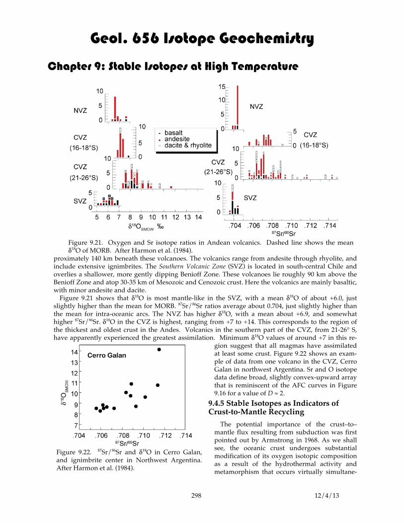
proximately 140 km beneath these volcanoes. The volcanics range from andesite through rhyolite, and include extensive ignimbrites. The Southern Volcanic Zone (SVZ) is located in south-central Chile and overlies a shallower, more gently dipping Benioff Zone. These volcanoes lie roughly 90 km above the Benioff Zone and atop 30-35 km of Mesozoic and Cenozoic crust. Here the volcanics are mainly basaltic, with minor andesite and dacite. Figure 9.21 shows that δ18O is most mantle-like in the SVZ, with a mean δ18O of about +6.0, just slightly higher than the mean for MORB. 87Sr/86Sr ratios average about 0.704, just slightly higher than the mean for intra-oceanic arcs. The NVZ has higher δ18O, with a mean about +6.9, and somewhat higher 87Sr/86Sr. δ18O in the CVZ is highest, ranging from +7 to +14. This corresponds to the region of the thickest and oldest crust in the Andes. Volcanics in the southern part of the CVZ, from 21-26° S, have apparently experienced the greatest assimilation. Minimum δ18O values of around +7 in this re-
gion suggest that all magmas have assimilated at least some crust. Figure 9.22 shows an exam-ple of data from one volcano in the CVZ, Cerro Galan in northwest Argentina. Sr and O isotope data define broad, slightly convex-upward array that is reminiscent of the AFC curves in Figure 9.16 for a value of D ≈ 2.
9.4.5 Stable Isotopes as Indicators of Crust-to-Mantle Recycling
The potential importance of the crust–to–mantle flux resulting from subduction was first pointed out by Armstrong in 1968. As we shall see, the oceanic crust undergoes substantial modification of its oxygen isotopic composition as a result of the hydrothermal activity and metamorphism that occurs virtually simultane-
Figure 9.22. 87Sr/86Sr and δ18O in Cerro Galan, and ignimbrite center in Northwest Argentina. After Harmon et al. (1984).
Figure 9.21. Oxygen and Sr isotope ratios in Andean volcanics. Dashed line shows the mean δ18O of MORB. After Harmon et al. (1984).

Geol. 656 Isotope Geochemistry
Chapter 9: Stable Isotopes at High Temperature
299 12/4/13
ously with formation of the oceanic crust and as a re-sult of low-temperature reactions with seawater. The hydrothermal activity tends to lower the δ18O of the middle and lower oceanic crust, while the low-temperature weathering raises the δ18O of the upper oceanic crust. As we’ll discuss in a subsequent section, there is little or no net change in oxygen isotope com-position of the oceanic crust as a result of these proc-esses. Thus subduction of the crystalline portion of the oceanic crust should have no net effect on the oxygen isotopic composition of the mantle as a whole, but it might increase isotopic heterogeneity. The subduction process may influence the compo-sition of the subcontinental lithosphere. As may be seen in Figure 9.23, eclogite* xenoliths from the Roberts Vic-tor Mine (South Africa) kimberlite have remarkably variable oxygen isotope compositions (MacGregor and Manton (1986). The range in δ18O is similar to that of “mature” oceanic crust (i.e., subsequent to hy-drothermal low temperature metamorphism), and con-trasts with the homogeneity of olivines in peridotite xenoliths (Figure 9.6), many of which also come from
kimberlites. Since eclogites are the high pressure equivalent of basalts, this suggests the ecolgites come from subducted oceanic crust. Further evidence to this effect is the correlation observed between O isotope ratios, Sr isotope ratios, and K and Rb concentrations, as these will also be affected by metamor-phism of the oceanic crust. Geo-barometry indicates these eclogites last equilibrated at depths of 165-190 km. Radiogenic isotope evi-dence suggests they are 2.47 Ga old. We examined the radiogenic iso-tope evidence for mantle hetero-geneity in Chapter 6. One inter-pretation is that this heterogeneity results from recycling of oceanic crust and sediment into the mantle. Since sediment, and, to a lesser degree, oceanic crust (as we shall see in the next section) differ in
* Eclogite is a rock consisting primarily of Na-rich pyroxene and garnet that forms only at high pressures. Composi-tionally these eclogites are similar to basalts, as are most.
Figure 9.23. Oxygen isotope ratios in eclogite xenoliths from the Roberts Victor Mine kim-berlite.
Figure 9.24. δ18O in olivines from oceanic island basalts and MORB. See Section 6.4 for the definition of EM1, EM2, and HIMU. Shaded areas shows the range of δ18O in upper man-tle peridotites (e.g., Figure 21.6). From Eiler et al. (1997).

Geol. 656 Isotope Geochemistry
Chapter 9: Stable Isotopes at High Temperature
300 12/4/13
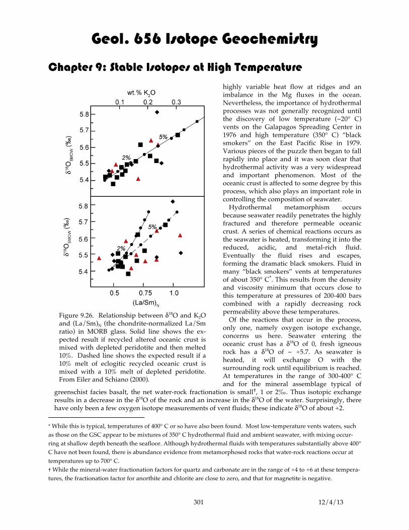
thier oxygen isotopic compositions from normal mantle material, we might expect this recycling to produce variations in O isotope composition of basalts. As Figure 9.24 shows, this is indeed observed. EM2 basalts (defined by their radiogenic isotopic compositions as shown in Figures 6.11 and 6.12) show systematically higher δ18O than MORB, while HIMU and low 3He/4He basalts (many HIMU basalts have low 3He/4He) have systematically low δ18O. It is in EM2 basalts, such as those from Samoa the Society Islands, where the best evidence for a recycled sedimentary compon-ent is seen (e.g. Figure 6.18). As we noted in Chapter 6, extremely radiogenic Sr was reported in lavas from Samoa by Jackson et al. (2007). Workman et al. (2008) found that δ18O was well correlated with 87Sr/86Sr in these lavas (Figure 9.25), further strengthening the case that the Samoan plume contains anciently subducted sediment. One ad-vantage of oxygen isotope ratios is that most rocks have rather similar oxygen concentrations. Thus, as-suming isotopic compositions of the end-members, we can easily calculate the fraction of each in a mix-ture. Workman et al. (2008) considered two models: one is which mantle (with olivine δ18O = +5.2‰ and 87Sr/86Sr ≈ 0.7045) mixes with anciently subducted upper continental crust (δ18O = +10‰, 87Sr/86Sr = 0.75), the other in which depleted mantle mixes with anciently subducted marine sediment (δ18O = +25‰, 87Sr/86Sr = 0.75). The curve for the latter mixing model is shown in Figure 9.25: up to about 2% sediment in the mixture would explain the isotopic compositions observed. Some Samoan lavas have even more radiogenic Sr, but those lack olivine phenocrysts and were not analyzed in this study. Ex-trapolating the model to those compositions implies their source contains 5 to 8% sediment. Even among MORB there is a correlation between incompatible element enrichment and δ18O (Figure 9.26). Since δ18O should be effectively insensitive to the extent of partial melting and fractional crystalli-zation, this correlation is likely to reflect a correlation between these properties in the MORB source. Since O isotope ratios can be changed only at low temperatures near the Earth’s surface, Eiler and Schi-ano (2000) interpret this as evidence of a recycled component in MORB.
9.5 OXYGEN ISOTOPES IN HYDROTHERMAL SYSTEMS 9.5.1 Ridge Crest Hydrothermal Activity and Metamorphism of the Oceanic Crust
Early studies of “greenstones” dredged from mid-ocean ridges and fracture zones revealed they were depleted in 18O relative to fresh basalts. Partitioning between of oxygen isotopes between various min-erals, such as carbonates, epidote, quartz and chlorite, in these greenstones suggested they had equili-brated at about 300° C (Muehlenbachs and Clayton, 1972). This was the first, but certainly not the only, evidence that the oceanic crust underwent hydrothermal metamorphism at depth. Other clues included
Figure 9.25. Oxygen and strontium isotope ratios in lavas from the Samoan archipelago (Savaii and Upolu are islands, the remainder are seamounts). Also shown is the mixing curve of the sedi-ment_mantle mixing model of Workman et al. (2008). After Workman et al. (2008).
Geol. 656 Isotope Geochemistry
Chapter 9: Stable Isotopes at High Temperature
301 12/4/13
highly variable heat flow at ridges and an imbalance in the Mg fluxes in the ocean. Nevertheless, the importance of hydrothermal processes was not generally recognized until the discovery of low temperature (~20° C) vents on the Galapagos Spreading Center in 1976 and high temperature (350° C) “black smokers” on the East Pacific Rise in 1979. Various pieces of the puzzle then began to fall rapidly into place and it was soon clear that hydrothermal activity was a very widespread and important phenomenon. Most of the oceanic crust is affected to some degree by this process, which also plays an important role in controlling the composition of seawater. Hydrothermal metamorphism occurs because seawater readily penetrates the highly fractured and therefore permeable oceanic crust. A series of chemical reactions occurs as the seawater is heated, transforming it into the reduced, acidic, and metal-rich fluid. Eventually the fluid rises and escapes, forming the dramatic black smokers. Fluid in many “black smokers” vents at temperatures of about 350° C*. This results from the density and viscosity minimum that occurs close to this temperature at pressures of 200-400 bars combined with a rapidly decreasing rock permeability above these temperatures. Of the reactions that occur in the process, only one, namely oxygen isotope exchange, concerns us here. Seawater entering the oceanic crust has a δ18O of 0, fresh igneous rock has a δ18O of ~ +5.7. As seawater is heated, it will exchange O with the surrounding rock until equilibrium is reached. At temperatures in the range of 300-400° C and for the mineral assemblage typical of
greenschist facies basalt, the net water-rock fractionation is small†, 1 or 2‰. Thus isotopic exchange results in a decrease in the δ18O of the rock and an increase in the δ18O of the water. Surprisingly, there have only been a few oxygen isotope measurements of vent fluids; these indicate δ18O of about +2.
* While this is typical, temperatures of 400° C or so have also been found. Most low-temperature vents waters, such as those on the GSC appear to be mixtures of 350° C hydrothermal fluid and ambient seawater, with mixing occur-ring at shallow depth beneath the seafloor. Although hydrothermal fluids with temperatures substantially above 400° C have not been found, there is abundance evidence from metamorphosed rocks that water-rock reactions occur at temperatures up to 700° C. † While the mineral-water fractionation factors for quartz and carbonate are in the range of +4 to +6 at these tempera-tures, the fractionation factor for anorthite and chlorite are close to zero, and that for magnetite is negative.
Figure 9.26. Relationship between δ18O and K2O and (La/Sm)N (the chondrite-normalized La/Sm ratio) in MORB glass. Solid line shows the ex-pected result if recycled altered oceanic crust is mixed with depleted peridotite and then melted 10%. Dashed line shows the expected result if a 10% melt of eclogitic recycled oceanic crust is mixed with a 10% melt of depleted peridotite. From Eiler and Schiano (2000).

Geol. 656 Isotope Geochemistry
Chapter 9: Stable Isotopes at High Temperature
302 12/4/13
At the same time hydrothermal metamorphism occurs deep in the crust, low-temperature weathering proceeds at the surface. This also involves isotopic exchange. However, for the temperatures (~2° C) and minerals produced by these reactions (smectites, zeolites, etc.), fractionations are quite large (some-thing like 20‰). The result of these reactions is to increase the δ18O of the shallow oceanic crust and de-crease the δ18O of seawater. Thus the effects of low temperature and high temperature reactions are opposing. Muehlenbachs and Clayton (1976) and Muehlenbachs and Furnas (2003) have argued that these op-posing reactions actually buffered the isotopic composition of seawater at a δ18O of ~0. According to them, the net of low and high temperature fractionations was about +6, just the observed difference be-tween the oceanic crust and the oceans. Thus, the oceanic crust ends up with an average δ18O value about the same as it started with, and the net effect on seawater must be close to zero also. Could this be coincidental? One should always be suspicious of apparent coincidences in science, and they were. Let’s think about this a little. Let’s assume the net fractionation is 6, but suppose the δ18O of the ocean was –10 rather than 0. What would happen? Assuming a sufficient amount of oceanic crust available and a simple batch reaction with a finite amount of water, the net of high and low temperature basalt-seawater reactions would leave the water with δ18O of –10 + 6 = –4. Each time a piece of oceanic crust is allowed to equilibrate with seawater, the δ18O of the ocean will increase a bit. If the process is repeated enough, the δ18O of the ocean will eventually reach a value of 6 – 6 = 0. Actually, what is required of seawater–oceanic crust interaction to maintain the δ18O of the ocean at 0‰ is a net increase in isotopic composition of seawater by perhaps 1–2‰. This is because low-temperature continental weathering has the net effect of decreasing the δ18O of the hydrosphere. This is what Muehlenbachs and Clayton proposed. The “half-time”, defined as the time required for the disequilibrium to decrease by half, for this proc-ess, has been estimated to be about 46 Ma. For example, if the equilibrium value of the ocean is 0 ‰ and the actual value is -2 ‰, the δ18O of the ocean should increase to –1 ‰ in 46 Ma. It would then re-quire another 46 Ma to bring the oceans to a δ18O of –0.5‰, etc. Over long time scales, this should keep the isotopic composition of oceanic crust constant. We’ll see in the next chapter that the oxygen isotopic composition of the ocean varies on times scales of thousands to tens of thousands of years due to changes in ice volume. The isotopic exchange with oceanic crust is much too slow to dampen these short-term variations. That water-rock interaction pro-duces essentially no net change in the isotopic composition of the oce-anic crust, and therefore of seawater was apparently confirmed by the first thorough oxygen isotope study of an ophiolite by Gregory and Tay-lor (1981). Their results for the Samail Ophiolite in Oman are shown in Figure 9.26. As expected, they found the upper part of the crust had higher δ18O than fresh MORB and while the lower part of the section had δ18O lower than MORB. Their es-timate for the δ18O of the entire sec-tion was +5.8, which is essentially identical to fresh MORB. At Ocean Drilling Project (ODP) Site 1256 in the equatorial eastern the oceanic
Figure 9.27. δ18O of the Samail Ophiolite in Oman as a func-tion of stratigraphic height. After Gregrory and Taylor (1981).

Geol. 656 Isotope Geochemistry
Chapter 9: Stable Isotopes at High Temperature
303 12/4/13
crust was cored to a depth of 1500 m, just penetrating into the gabbroic layer. Oxygen isotope ratios show much the same pattern as the Samail ophiolite (Figure 9.28), with heavy oxygen in the volcanic zone and light oxygen in the dikes and gabbros. The shift in isotopic composition is coincident with a shift in the style of alteration from low- to high-temperature apparent from petrographic examination. If the Muehlenbachs and Clayton hypothesis is correct, and assuming a steady-state tectonic environment, the δ18O of the oceans should remain constant over geologic time. Whether it has or not, is controversial. Based on analyses of marine carbonates, Jan Veizer and his colleagues have argued that it is not (e.g., Veizer et al., 1999). The basis of their argument was that that δ18O in marine carbonates increases over Phanerozoic time (Figure 9.29). More recently, however, Came et al. (2007) have used isotopic clumping analysis to calculate the isotopic composition of seawater from these Silurian and Carboniferous marine carbonates and found that seawater at the time indeed had values close to modern ones, implying the Muehlenbachs and Clayton hypothesis is correct. We’ll consider this in more detail in Chapter 11.
9.5.2 Meteoric Geothermal Systems Hydrothermal systems occur not only in the ocean, but just about everywhere that magma is intruded into the crust. In the 1950’s a debate raged about the rate at which the ocean and atmosphere were created by degassing of the Earth’s interior. W. W. Rubey assumed that water in hydrothermal systems such as Yellowstone was magmatic and argued that the ocean and atmosphere were created quite gradually through magmatic degassing. Rubey turned out to be wrong about hydrothermal systems. One of the first of many important contributions of stable isotope geo-chemistry to understanding hydrothermal systems was the demonstration by Craig (1963) that water in these systems was meteoric, not magmatic. The argument is based upon the data shown in Figure 9.30. For each geothermal system, the δD of the “chloride” type geothermal waters is the nearly same as the local precipitation and groundwater, but the δ18O is shifted to higher values. The shift in δ18O results from “high” temperature (~300°C) reaction of the local meteoric water with hot rock. However, because concentration of hydrogen in rocks is nearly 0 (more precisely because ratio of the mass of hydrogen in the water to mass of hydrogen in the reacting rocks is extremely high), there is essentially no change in the hydrogen isotopic composition of the water. If the water involved in these systems was magmatic, it would not have the same δD as local meteoric water (though it is possible that these systems contain a few percent magmatic water).
Figure 9.28. Oxygen isotope ratios measured in cores from ODP Site 1256 in the equatorial east-ern Pacific. Cross-hatched area is the lava-dike transition zone. The volcanic section has mostly elevated δ18O as a consequence of low-temperature interaction with seawater while the dikes and gabbros have mostly lowered δ18O as a consequence of hydrothermal interaction. Data from Gao et al. (2012).

Geol. 656 Isotope Geochemistry
Chapter 9: Stable Isotopes at High Temperature
304 12/4/13
Acidic, sulfide-rich water from these systems does have δD that is different from local meteoric wa-ter. This shift occurs when hydrogen isotopes are fractionated during boiling of geothermal waters. The steam produced is enriched in sulfide, accounting for their acidic character. The water than con-denses from this steam the mixes with meteoric water to produce the mixing lines observed.
9.5.3 Water-Rock Reaction: Theory Very often in geology it is difficult to observe the details of processes occurring today and our under-standing of many of Earth processes comes from observing the effects these processes have had in the past, i.e., the record they have left in the rocks. So it is with hydrothermal systems. In present systems, we very often can observe only the water venting, we cannot observe the reactions with rocks or the pattern of circulation. However, these, as well as temperatures involved and water-rock ratios, can be inferred from the imprint left by ancient hydrothermal systems. Estimating temperatures at which ancient hydrothermal systems operated is a fairly straightforward application of isotope geothermometry, which we have already discussed. If we can measure the oxy-gen (or carbon or sulfur) isotopic composition of any two phases that were in equilibrium, and if we know the fractionation factor as a function of temperature for those phases, we can estimate the tem-perature of equilibration. We will focus now on water-rock ratios, which may also be estimated using stable isotope ratios. For a closed hydrothermal system, we can write two fundamental equations. The first simply de-scribes equilibrium between water and rock:
Δ = δwf −δ r
f 9.11 where we use the subscript w to indicate water, and r to indicate rock. The superscript f indicates the final value. So equation 9.10 just says that the difference between the final isotopic composition of wa-ter and rock is equal to the fractionation factor (we implicitly assume equilibrium). The second equation is just a statement of mass balance for a closed system: the amount of the isotope present before reac-tion must be the same as after reaction:
Figure 9.29. δ18O in marine carbonates (brachiopods, belemites, oysters, and foraminifera shells) over Phanerozoic time. After Veizer et al. (1999).

Geol. 656 Isotope Geochemistry
Chapter 9: Stable Isotopes at High Temperature
305 12/4/13
cwWδwi + crRδr
i = cwWδwf + crRδr
f 9.12 where c indicates concentration (we assume concentrations do not change, which is valid for oxygen, but not generally valid for other elements), W indicates the mass of water involved, R the mass of rock involved, and the superscript i denotes the initial isotope ratio. Substituting equation 9.10 and rearranging, we derive the following equation:
W
R=
δrf − δr
i
δwi − δr
f − Δcrcw
9.13
The term on the left is the ratio of water to rock in the reaction. Notice that the r.h.s. does not include the final isotopic composition of the water, information that we would generally not have. The initial oxygen isotope composition of the water can be estimated in various ways. For example, we can deter-mine the hydrogen isotopic composition (of rocks) and from that determine the oxygen isotope compo-sition using the δD– δ18O meteoric water line. The initial δ18O of rock can generally be inferred from un-altered samples, and the final isotopic composition of the rock can be measured. The fractionation fac-tor can be estimated if we know the temperature and the phases in the rock. For oxygen, the ratio of concentration in the rock to water will be close to 0.5 in all cases. Equation 9.13 is for a closed system, i.e., a batch reaction where we equilibrate W grams of water with R grams of rock. That is not very geo-logically realistic. In fact, a completely open system, where water makes one pass through hot rock, would be more realistic. In this case, we might suppose that a small parcel of water, dW, passes through the system and induces and in-cremental change in the isotopic compo-sition of the rock, dδr. In this case, we can write:
Rcrdδr = δwi − Δ + δr[ ]( )cwdW 9.14
This equation states that the mass of iso-tope exchanged by the rock is equal to the mass of isotope exchanged by the wa-ter (we have substituted ∆ + δr for δf
w ). Rearranging and integrating, we have:
�
WR
= lnδr
f −δri
−δrf +δw
i −Δ+1
⎛
⎝ ⎜
⎞
⎠ ⎟ crcw
9.15
Thus it is possible to deduce the water rock ratio for an open system as well as a closed one. Using this kind of approach, Gregory and Taylor (1981) estimated water/rock ratios of ≤ 0.3 for the gabbros of the Oman ophiolite. It should be empha-sized, however, that this can be done with other isotope systems as well. For example, McCulloch et al. (1981) used Sr isotope ratios to estimate water/rock ra-
Figure 9.30. δD and δ18O in meteoric hydrothermal systems. Closed circles show the composition of meteoric water in the vicinity of Yellowstone, Steamboat Springs (Colorado), Mt. Lassen (California), Iceland, Larderello (Italy), and The Geysers (California), and open circles show the isotopic composition of chloride-type geothermal waters at those locations. Open triangles show the location of acidic, sul-fide-rich geothermal waters at those locations. Solid lines connect the meteoric and chloride waters, dashed lines con-nect the meteoric and acidic waters. The “Meteoric Water Line” shows the correlation between δD and δ18O observed in precipitation shown in Figure 8.11.

Geol. 656 Isotope Geochemistry
Chapter 9: Stable Isotopes at High Temperature
306 12/4/13
tios varying from 0.5 to 40 for different parts of the Oman ophiolite.
9.5.4 The Skaergaard Intrusion A classic example of a meteoric hydro-thermal system is the Early Tertiary Skaer-gaard intrusion in East Greenland. The Skaergaard has been studied for nearly 75 years as a classic mafic layered intrusion. Perhaps ironically, the initial motivation for isotopic study of the Skaergaard was deter-mination of primary oxygen and hydrogen isotopic compositions of igneous rocks. The results, however, showed that the oxygen isotope composition of the Skaergaard has been pervasively altered by hydrothermal fluid flow. This was the first step in another important contribution of stable isotope geo-chemistry, namely the demonstration that most igneous intrusions have reacted exten-sively with water subsequent to crystalliza-tion. Figure 9.31 shows a map of the Skaergaard with contours of δ18O superimposed on it. Figure 9.31 shows a restored cross section of the intrusion with contours of δ18O. There are several interesting features. First, it is clear that circulation of water was strongly con-trolled by permeability. The impermeable basement gneiss experienced little exchange, as did the part of the intrusion beneath the contact of the gneiss with the overlying ba-salt. The basalt, which is typically highly fractured, is quite permeable and allowed
water to flow freely through it and into the intrusion. Figures 9.31 and 9.32 de-fine zones of low δ18O, which are the re-gions of hydrothermal upwelling. Water was apparently drawn into the sides of the intrusion and then rose above. This is just the sort of pattern observed with finite element models of fluid flow through the intrusion.
Figure 9.31. Restored cross-section of the Skaergaard in-trusion with contours of δ18O.
Figure 9.31. Oxygen isotope variations in the Skaer-gaard Intrusion. LZ, MZ, and UZ refer to the ‘lower zone, ‘middle zone’ and ‘upper zone’ of the intrusion, which dips 20-25° to the southeast. UBZ refer to the ‘upper border group’. The δ18O = +6 contour corre-sponds more or less to the trace of the gneiss-basalt contact through the intrusion (SW to NE). The gneiss is essentially impermeable, while the basalt is highly fractured. Thus most water flow was above this con-tact, and the gabbro below it retained its original ‘man-tle’ isotopic signature (+6). After Taylor (1974).

Geol. 656 Isotope Geochemistry
Chapter 9: Stable Isotopes at High Temperature
307 12/4/13
Calculated water-rock ratios for the Skaergaard were 0.88 in the basalt, 0.52 in the upper part of the intrusion and 0.003 for the gneiss, demonstrat-ing the importance of the basalt in conduction the water into the intru-sion and the inhibiting effect of the gneiss. Models of the cooling history of the intrusion suggest that each cm3 of rock was exposed to between 105 and 5 × 106 cm3 of water over the 500,000 year cooling history of the in-trusion. This would seem to conflict with the water/rock ratios estimated from oxygen isotopes. The difference is a consequence of each cm3 of water flowing through many cm3 of rock, but not necessarily reacting with it. Once water had flowed through enough grams of rock to come to iso-topic equilibrium, it would not react further with the rock through which it subsequently flowed (assuming constant temperature and mineral-ogy). Thus it is important to distin-
guish between W/R ratios calculated from isotopes, which reveal only the mass (or molar) ratio of water and rock in the net reaction, to flow models. Nevertheless, the flow models demonstrate that each gram of rock in such a system is exposed to an enormous amount of water. Figure 9.33 is a cartoon illustrat-ing the hydrothermal system deduced from the oxygen isotope study.
9.5.5 Oxygen Isotopes and Mineral Exploration Oxygen isotope studies can be a valuable tool in mineral exploration. Mineralization is very often (though not exclusively) associated with the region of greatest water flux, such as areas of upward moving hot water above intrusions. Such areas are likely to have the lowest values of δ18O. To under-stand this, let’s solve equ. 9.15, the final value of δ18O:
δ r
f = (δ ri −δw
i −∆)e−(W /R)(cw /cr ) +δwi +∆ 9.16
If we assume a uniform initial isotopic composition of the rocks and the water, then all the terms on the r.h.s. are constants except W/R and ∆, which is a function of temperature. Thus the final values of δ18O, i.e., the values we measure in an area such as the Skaergaard, are functions of the temperature of equilibration, and an exponential function of the W/R ratio. Figure 9.34 shows δ18Of
r plotted as a func-tion of W/R and ∆, where δ18Oi
r is assumed to be +6 and δ18Oiw is assumed to be -13.
Figure 9.35 shows another example of the δ18O imprint of an ancient hydrothermal system: the Bo-hemia mining district in Lane County, Oregon, where Tertiary volcanic rocks of the Western Cascades have been intruded by a series of dioritic plutons. Approximately $1,000,000 worth of gold was re-moved from the region between 1870 and 1940. δ18O contours form a bull’s eye pattern, and the region of low δ18O corresponds roughly with the area of prophylitic (i.e., greenstone) alteration. Notice that this region is broader than the contact metamorphic aereole. The primary area of mineralization occurs within the δ18O < 0 contour. In this area relatively large volumes of gold-bearing hydrothermal solu-tion, cooled, perhaps to mixing with ground water, and precipitated gold. This is an excellent example
Figure 9.33. Cartoon illustrating the hydrothermal system in the Skaergaard intrusion. After Taylor (1968).
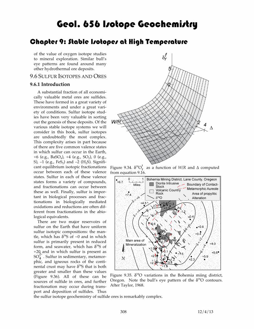
Geol. 656 Isotope Geochemistry
Chapter 9: Stable Isotopes at High Temperature
308 12/4/13
of the value of oxygen isotope studies to mineral exploration. Similar bull’s eye patterns are found around many other hydrothermal ore deposits.
9.6 SULFUR ISOTOPES AND ORES 9.6.1 Introduction
A substantial fraction of all economi-cally valuable metal ores are sulfides. These have formed in a great variety of environments and under a great vari-ety of conditions. Sulfur isotope stud-ies have been very valuable in sorting out the genesis of these deposits. Of the various stable isotope systems we will consider in this book, sulfur isotopes are undoubtedly the most complex. This complexity arises in part because of there are five common valence states in which sulfur can occur in the Earth, +6 (e.g., BaSO4), +4 (e.g., SO2), 0 (e.g., S), –1 (e.g., FeS2) and –2 (H2S). Signifi-cant equilibrium isotopic fractionations occur between each of these valence states. Sulfur in each of these valence states forms a variety of compounds, and fractionations can occur between these as well. Finally, sulfur is impor-tant in biological processes and frac-tionations in biologically mediated oxidations and reductions are often dif-ferent from fractionations in the abio-logical equivalents. There are two major reservoirs of sulfur on the Earth that have uniform sulfur isotopic compositions: the man-tle, which has δ34S of ~0 and in which sulfur is primarily present in reduced form, and seawater, which has δ34S of +20 and in which sulfur is present as SO2-
4 . Sulfur in sedimentary, metamor-phic, and igneous rocks of the conti-nental crust may have δ34S that is both greater and smaller than these values (Figure 9.36). All of these can be sources of sulfide in ores, and further fractionation may occur during trans-port and deposition of sulfides. Thus the sulfur isotope geochemistry of sulfide ores is remarkably complex.
Figure 9.34. δ18Of
r as a function of W/R and ∆ computed from equation 9.16.
Figure 9.35. δ18O variations in the Bohemia miing district, Oregon. Note the bull’s eye pattern of the δ18O contours. After Taylor, 1968.

Geol. 656 Isotope Geochemistry
Chapter 9: Stable Isotopes at High Temperature
309 12/4/13
9.6.2 Sulfur Isotope Fractionations in Magmatic Processes
Sulfur is present in peridotites as trace sulfides, and that is presumably its primary form in the mantle. At temperatures above about 400 °C, H2S and SO2 are the stable forms of sulfur in fluids and melts. In basaltic melts, sulfur occurs pre-dominantly as dissociated H2S: HS–. It is unlikely that significant fractionation occurs between these forms during melting. Indeed, as we have seen, the mean δ34S in basalts (~+0.1) is close to the value in meteorites, which is presumably also the mantle value. The solubility of H2S in silicate melts is related to the Fe content, decreasing with decreasing Fe. The solubility of H2S in basalt ap-pears to be only slightly less than that of water, so that under moderate pressure, essentially all sulfur will remain dissolved in basaltic liquids.
As basalts rise into the crust, cool, and crystallize, several processes can affect the oxidation state and solubility of sulfur and the produce isotopic frac-tionations. First, the decreasing pressure results in some of the sulfide partitioning into the gas (or fluid) phase. In addition, H2 can be lost from the melt through diffusion. This increases the ƒO2 of the melt, and as result, some of the sulfide will be oxi-dized to SO2, which is very much less soluble in silicate melts than H2S. Decreasing Fe content as a consequence of fractional crystallization will also decrease the solubility of S in the melt, increasing its concentration in a coexisting fluid or gas phase. Isotope fractionation will occur between the three species (dissolved HS–, H2S, SO2). The isotopic composition of the fluid (gas) will differ from that of the melt, and can be computed as:
�
δ 34Sfluid =δ 34Smelt −ΔHS−+ ΔSO2
RR+1
⎛ ⎝ ⎜
⎞ ⎠ ⎟ 9.17
where ∆HS is the fractionation factor between HS– and H2S, ∆SO2 is the fractionation factor between H2S and SO2, and R is the mole fraction ratio SO2/H2S and is given by:
�
R =XSO2
XH2S
=KνH2S
ƒO2
3/2
PfνH2OXH2O
νSO2
9.18
where ν are the fugacity or activity coefficients, Pf is the fluid pressure (generally equal to total pres-sure), ƒO2 is oxygen fugacity, and K is the equilib-rium constant for the reaction:
Figure 9.36. δ34SCDT in various geologic materials (after Hoefs, 1987).
Figure 9.37. Fractionation of sulfur isotopes be-tween fluid and melt (shown by dashed curves) as a function of oxygen fugacity and temperature for PH2O = 1 kB. Solid lines show equal concen-tration boundaries for quartz + magnetite ® fay-alite (QM-F), H2S ® SO2, and Magnetite ® Hema-tite (M-H). After Ohmoto and Rye (1979).

Geol. 656 Isotope Geochemistry
Chapter 9: Stable Isotopes at High Temperature
310 12/4/13
H2S(g) + 32 O2 ® H2O(g) + SO2(g) 9.19
Figure 9.37 shows the sulfur isotope fractionation between fluid and melt calculated from equations 9.17 and 9.18 as a function of function of temperature and ƒO2 for PH2O = 1 kB. At the temperatures and ƒO2 of most basalts, sulfur will be present primarily as H2S in the fluid (gas phase) and HS– in the melt. The fractionation between these species is small (~ 0.6 ‰), so the isotopic composition of fluid phase will not be very different that of the melt. For rhyolites and dacites, a significant fraction of the sulfur can be present as SO2, so that greater fractionation between melt and fluid is possible. An interesting feature of the above equations is that the fractionation between fluid and melt depends on the water pressure. Figure 9.37 is valid only for PH2O = 1 kB. A decrease in Pf or XH2O (the mole fraction of water in the fluid) will shift the SO2/H2S equal concentration boundary and the δ34S contours to lower ƒO2. Conversely, an increase the in the water content will shift to boundary toward higher ƒO2. Both the eruptions of El Chichón in 1983 and Pinatubo in 1991 release substantial amounts of SO2, which resulted in global climate cooling. The SO2–rich nature of these eruptions is thought to result from mixing of a mafic, S-bearing magma with a more oxidized dacitic magma, which resulted in oxi-dation of the sulfur, and consequent increase of SO2 in the fluid phase. There are a number of other processes that affect the solubility and oxidation state of sulfur in the melt, and hence isotopic fractiona-tion. Wall rock reactions could lead to either oxidation or reduction of sulfur, crystallization of sulfides or sulfates could cause relatively small fractionations and additionally affect the SO2/H2S ratio of the fluid. Depending on the exact evolutionary path taken by the magma and fluid, δ34S of H2S may be up to –13‰ lower than that of the original magma. Thus variations in the isotopic composition of sulfur are possible even in a mantle-derived magma whose initial δ34S was that of the mantle (~ 0‰). Variabil-ity of sulfur isotopic compositions do, however, give some indication of the ƒO2 history of a magma. Constant δ34S of magmatic sulfides suggests ƒO2 remained below the SO2/H2S boundary; variability in isotopic composition suggests a higher ƒO2.
9.6.3 Sulfur Isotope Fractionation in Hydrothermal Systems Although some sulfide ore deposits are magmatic, most were deposited by precipitation from aque-ous solution at low to moderate temperature. At temperatures below about 400° C, sulfide species (H2S and HS–) are joined by sulfate (SO 4
2 − , HSO41− , KSO4
1− , NaSO 41− , CaSO4 and MgSO4) as the dominant
forms of aqueous sulfur. The ratio of sulfide to sulfate will depend on the oxidation state of the fluid. Small fractionations occur among the various sulfide and sulfate species, but there is a major fractiona-tion between sulfide and sulfate. Neglecting the small fractionation between H2S and HS– and among sulfate species, δ34SH2S of the fluid can be expressed as:
�
δ 34SH2S =δ 34Sfluid −ΔSO42− ×
′ R ′ R +1
⎛ ⎝ ⎜
⎞ ⎠ ⎟ 9.20
where ΔSO42− is the fractionation between H2S and SO4
2 − and R´ is the molar ratio of sulfide to sulfate:
�
′ R = ΣSO42−
ΣH2S 9.21
In general, R’ will be a function of ƒO2, pH, fluid composition and temperature. Figure 9.38 shows the
difference between δ34S in sulfide and δ34S in the total fluid as a function of pH and ƒO2. Only under
conditions of low pH and low ƒO2, will the δ34S of pyrite (FeS2) be the same as the δ34S of the fluid from
which it precipitated. For conditions of relatively high ƒO2 or high pH, substantial differences between
the δ34S of pyrite and the δ34S of the fluid from which it precipitated are possible. Figure 9.39 shows the difference between δ34S in sulfide and δ34S in the total fluid as a function of the sulfate/sulfide ratio (R´) and temperature. When the fluid is sulfide dominated, the δ34S of the sulfide and that of the bulk fluid
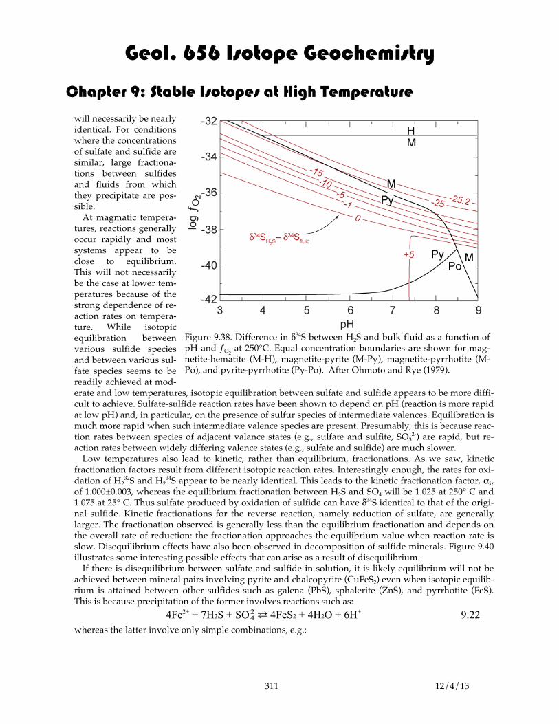
Geol. 656 Isotope Geochemistry
Chapter 9: Stable Isotopes at High Temperature
311 12/4/13
will necessarily be nearly identical. For conditions where the concentrations of sulfate and sulfide are similar, large fractiona-tions between sulfides and fluids from which they precipitate are pos-sible. At magmatic tempera-tures, reactions generally occur rapidly and most systems appear to be close to equilibrium. This will not necessarily be the case at lower tem-peratures because of the strong dependence of re-action rates on tempera-ture. While isotopic equilibration between various sulfide species and between various sul-fate species seems to be readily achieved at mod-erate and low temperatures, isotopic equilibration between sulfate and sulfide appears to be more diffi-cult to achieve. Sulfate-sulfide reaction rates have been shown to depend on pH (reaction is more rapid at low pH) and, in particular, on the presence of sulfur species of intermediate valences. Equilibration is much more rapid when such intermediate valence species are present. Presumably, this is because reac-tion rates between species of adjacent valance states (e.g., sulfate and sulfite, SO3
2-) are rapid, but re-action rates between widely differing valence states (e.g., sulfate and sulfide) are much slower. Low temperatures also lead to kinetic, rather than equilibrium, fractionations. As we saw, kinetic fractionation factors result from different isotopic reaction rates. Interestingly enough, the rates for oxi-dation of H2
32S and H234S appear to be nearly identical. This leads to the kinetic fractionation factor, αk,
of 1.000±0.003, whereas the equilibrium fractionation between H2S and SO4 will be 1.025 at 250° C and 1.075 at 25° C. Thus sulfate produced by oxidation of sulfide can have δ34S identical to that of the origi-nal sulfide. Kinetic fractionations for the reverse reaction, namely reduction of sulfate, are generally larger. The fractionation observed is generally less than the equilibrium fractionation and depends on the overall rate of reduction: the fractionation approaches the equilibrium value when reaction rate is slow. Disequilibrium effects have also been observed in decomposition of sulfide minerals. Figure 9.40 illustrates some interesting possible effects that can arise as a result of disequilibrium. If there is disequilibrium between sulfate and sulfide in solution, it is likely equilibrium will not be achieved between mineral pairs involving pyrite and chalcopyrite (CuFeS2) even when isotopic equilib-rium is attained between other sulfides such as galena (PbS), sphalerite (ZnS), and pyrrhotite (FeS). This is because precipitation of the former involves reactions such as: 4Fe2+ + 7H2S + SO4
2 ® 4FeS2 + 4H2O + 6H+ 9.22 whereas the latter involve only simple combinations, e.g.:
Figure 9.38. Difference in δ34S between H2S and bulk fluid as a function of pH and ƒO2
at 250°C. Equal concentration boundaries are shown for mag-netite-hematite (M-H), magnetite-pyrite (M-Py), magnetite-pyrrhotite (M-Po), and pyrite-pyrrhotite (Py-Po). After Ohmoto and Rye (1979).

Geol. 656 Isotope Geochemistry
Chapter 9: Stable Isotopes at High Temperature
312 12/4/13
Zn2+ + H2S + ® ZnS + 2H+ 9.23
9.6.4 Isotopic Composition of Sulfide Ores A number of important sulfide deposits were apparently produced by reduction of sulfate that was ultimately de-rived from seawater. The expected isotopic compositions of such deposits are shown in Figure 9.41. The isotopic com-position of these sulfides depends on the reduction mecha-nism, temperature, and whether the system was open or closed to sulfate and sulfide. At temperatures less than 50° C, the only mechanism for reduction of sulfate is bacterial. Optimal temperatures for such reduction are around 30 to 50° C. Deep euxinic basins such as the Black Sea are good examples of systems that are open to SO4 but closed to H2S and where reduction is bacterial. In these cases, reduction occurs slowly at the bottom, but SO4 is continuously sup-plied from the water mass above. In such environments, sulfides appear to have a δ34S of 40 to 60‰ less than that of contemporaneous seawater (the sulfur isotopic composition of seawater has varied through time). A good example of
such a deposit is the Kupfershiefer in Germany, where the most common δ34S is about –40‰, which is about 50‰ less than Permian seawater (+10‰). In systems closed to SO4 but open to H2S, the process is similar to Rayleigh distillation. This would be the case, for example, where sulfate reduction oc-curs much more rapidly than sulfate is supplied to the system, but sulfide is ef-fectively lost from the system by crys-tallization of sulfide minerals. The com-position of the sulfate, as a function of the fraction of sulfate remaining, ƒ, is given by:
δ 34S
SO42− = δ 34S
SO42−
0
+1000(ƒ1−α −1) 9.24
The composition of the sulfide at any time, t, is related to that of sulfate by:
Figure 9.39. Difference in δ34S between H2S and bulk fluid as a function of tem-perature and sulfate/sulfide ratio in a pH neutral fluid. Equal concentration boundaries M: magnetite, H: hematite, Py: pyrite, Po: pyrrhotite, Bn: bornite (Cu5FeS4), Cp: chalcopyrite. After Oh-moto and Rye (1979).
Figure 9.40. Isotopic relationships between coexisting H2S and SO4
-2 as a function of sulfate/sulfide ratio. (a) Equilib-
rium conditions at 250° C where δ34Sfluid = 0 ‰. (b) Non-equilibrium oxidation of H2S. Isotopic composition of H2S remains constant, but that of sulfate changes due to addition of sulfate derived from non-equilibrium oxidation of H2S. (c) Non-equilibrium mixing of H2S-rich fluid A and SO4-rich fluid B. δ34SH2S remains constant (equilibrium fractionation is achieved during reduction), but δ34SSO4 varies due to addi-tion of sulfate derived from oxidation of sulfide. After Oh-moto and Rye (1979).
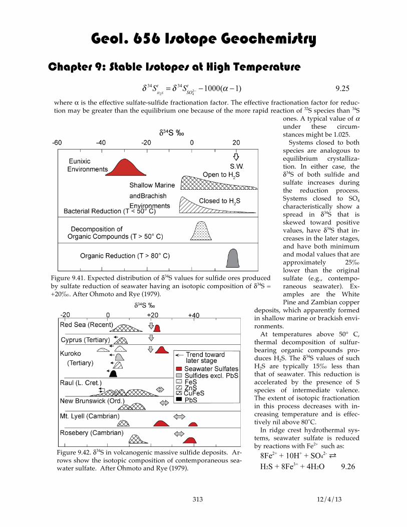
Geol. 656 Isotope Geochemistry
Chapter 9: Stable Isotopes at High Temperature
313 12/4/13
δ 34SH2S
t = δ 34SSO4
2−t −1000(α −1) 9.25
where α is the effective sulfate-sulfide fractionation factor. The effective fractionation factor for reduc-tion may be greater than the equilibrium one because of the more rapid reaction of 32S species than 34S
ones. A typical value of α under these circum-stances might be 1.025. Systems closed to both species are analogous to equilibrium crystalliza-tion. In either case, the δ34S of both sulfide and sulfate increases during the reduction process. Systems closed to SO4 characteristically show a spread in δ34S that is skewed toward positive values, have δ34S that in-creases in the later stages, and have both minimum and modal values that are approximately 25‰ lower than the original sulfate (e.g., contempo-raneous seawater). Ex-amples are the White Pine and Zambian copper
deposits, which apparently formed in shallow marine or brackish envi-ronments. At temperatures above 50° C, thermal decomposition of sulfur-bearing organic compounds pro-duces H2S. The δ34S values of such H2S are typically 15‰ less than that of seawater. This reduction is accelerated by the presence of S species of intermediate valence. The extent of isotopic fractionation in this process decreases with in-creasing temperature and is effec-tively nil above 80˚C. In ridge crest hydrothermal sys-tems, seawater sulfate is reduced by reactions with Fe2+ such as: 8Fe2+ + 10H+ + SO4
2- ® H2S + 8Fe3+ + 4H2O 9.26
Figure 9.41. Expected distribution of δ34S values for sulfide ores produced by sulfate reduction of seawater having an isotopic composition of δ34S = +20‰. After Ohmoto and Rye (1979).
Figure 9.42. δ34S in volcanogenic massive sulfide deposits. Ar-rows show the isotopic composition of contemporaneous sea-water sulfate. After Ohmoto and Rye (1979).
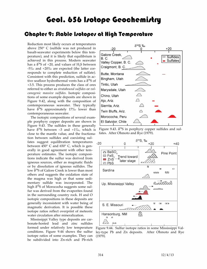
Geol. 656 Isotope Geochemistry
Chapter 9: Stable Isotopes at High Temperature
314 12/4/13
Reduction most likely occurs at temperatures above 250° C (sulfide was not produced in basalt-seawater experiments below this tem-perature), and it is likely that equilibrium is achieved in this process. Modern seawater has a δ34S of +20, and values of H2S between -5‰ and +20‰ are expected (the latter cor-responds to complete reduction of sulfate). Consistent with this prediction, sulfide in ac-tive seafloor hydrothermal vents has a δ34S of +3.5. This process produces the class of ores referred to either as stratabound sulfides or vol-canogenic massive sulfides. Isotopic composi-tions of some example deposits are shown in Figure 9.42, along with the composition of contemporaneous seawater. They typically have δ34S approximately 17‰ lower than contemporaneous seawater. The isotopic compositions of several exam-ple porphyry copper deposits are shown in Figure 9.43. The sulfides in these generally have δ34S between –3 and +1‰, which is close to the mantle value, and the fractiona-tion between sulfides and coexisting sul-fates suggest equilibration temperatures between 450° C and 650° C, which is gen-erally in good agreement with other tem-perature estimates. The isotopic composi-tions indicate the sulfur was derived from igneous sources, either as magmatic fluids or by dissolution of igneous sulfides. The low δ34S of Galore Creek is lower than most others and suggests the oxidation state of the magma was high or that some sedi-mentary sulfide was incorporated. The high δ34S of Morococha suggests some sul-fur was derived from the evaporites found in the surrounding country rock. H and O isotopic compositions in these deposits are generally inconsistent with water being of magmatic derivation. It is possible these isotope ratios reflect overprint of meteoric water circulation after mineralization. Mississippi Valley type deposits are car-bonate-hosted lead and zinc sulfides formed under relatively low temperature conditions. Figure 9.44 shows the sulfur isotope ratios of some examples. They can be subdivided into Zn-rich and Pb-rich
Figure 9.43. δ34S in porphyry copper sulfides and sul-fates. After Ohmoto and Rye (1979).
Figure 9.44. Sulfur isotope ratios in some Mississippi Val-ley-type Pb and Zn deposits. After Ohmoto and Rye (1979).
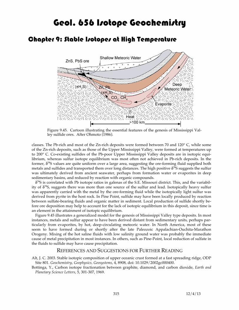
Geol. 656 Isotope Geochemistry
Chapter 9: Stable Isotopes at High Temperature
315 12/4/13
classes. The Pb-rich and most of the Zn-rich deposits were formed between 70 and 120° C, while some of the Zn-rich deposits, such as those of the Upper Mississippi Valley, were formed at temperatures up to 200° C. Co-existing sulfides of the Pb-poor Upper Mississippi Valley deposits are in isotopic equi-librium, whereas sulfur isotope equilibrium was most often not achieved in Pb-rich deposits. In the former, δ34S values are quite uniform over a large area, suggesting the ore-forming fluid supplied both metals and sulfides and transported them over long distances. The high positive δ34S suggests the sulfur was ultimately derived from ancient seawater, perhaps from formation water or evaporites in deep sedimentary basins, and reduced by reaction with organic compounds. δ34S is correlated with Pb isotope ratios in galenas of the S.E. Missouri district. This, and the variabil-ity of δ34S, suggests there was more than one source of the sulfur and lead. Isotopically heavy sulfur was apparently carried with the metal by the ore-forming fluid while the isotopically light sulfur was derived from pyrite in the host rock. In Pine Point, sulfide may have been locally produced by reaction between sulfate-bearing fluids and organic matter in sediment. Local production of sulfide shortly be-fore ore deposition may help to account for the lack of isotopic equilibrium in this deposit, since time is an element in the attainment of isotopic equilibrium. Figure 9.45 illustrates a generalized model for the genesis of Mississippi Valley type deposits. In most instances, metals and sulfur appear to have been derived distant from sedimentary units, perhaps par-ticularly from evaporites, by hot, deep-circulating meteoric water. In North America, most of these seem to have formed during or shortly after the late Paleozoic Appalachian-Ouchita-Marathon Orogeny. Mixing of the hot saline fluids with low salinity ground water was probably the immediate cause of metal precipitation in most instances. In others, such as Pine-Point, local reduction of sulfate in the fluids to sulfide may have cause precipitation.
REFERENCES AND SUGGESTIONS FOR FURTHER READING Alt, J. C. 2003. Stable isotopic composition of upper oceanic crust formed at a fast spreading ridge, ODP
Site 801. Geochemistry, Geophysics, Geosystems, 4, 8908, doi: 10.1029/2002gc000400. Bottinga, Y., Carbon isotope fractionation between graphite, diamond, and carbon dioxide, Earth and
Planetary Science Letters, 5, 301-307, 1969.
Figure 9.45. Cartoon illustrating the essential features of the genesis of Mississippi Val-ley sulfide ores. After Ohmoto (1986).
Geol. 656 Isotope Geochemistry
Chapter 9: Stable Isotopes at High Temperature
316 12/4/13
Came, R. E., Eiler, J. M., Veizer, J., Azmy, K., Brand, U. & Weidman, C. R. 2007. Coupling of surface temperatures and atmospheric CO2 concentrations during the Palaeozoic era. Nature, 449, 198-201, doi: 10.1038/nature06085.
Chacko, T., D. Cole and J. Horita,Equilibrium oxygen, hydrogen and carbon isotope fractionation facty-ors applicable to geologic systems, in J. W. Valley (ed.), Stable Isotope Geochemistry, , Mineralogical So-ciety of America, Washington, pp 1-61, 2001.
Chaussidon, M., S. M. F. Sheppard and A. Michard, Hydrogen, sulfur and neodymium isotope varia-tions in the mantle beneath the EPR at 12°50´N, in Stable Isotope Geochemistry: A Tribute to Samuel Ep-stein, edited by H. P. Taylor, J. R. O’Niel and I. R. Kaplan, p. 325-338, Geochemical Society, San Anto-nio, 1991.
Craig, H., The isotopic composition of water and carbon in geothermal areas, in Nuclear Geology on Geo-thermal Areas, ed. by E. Tongiorgi, p. 17-53, CNR Lab. Geol. Nucl., Pisa, 1963.
Criss, R. E. and H. P. Taylor, Meteoric-hydrothermal systems, in Stable Isotopes in High Temperature Geo-logical Processes, Reviews in Mineralogy 16, ed. by J. W. Valley, H. P. Taylor and J. R. O'Neil, p. 373-424, Mineral. Soc. Am., Washington, 1986.
DePaolo, D. J. 1981. Trace element and isotopic effects of combined wallrock assimilation and fractional crystallization. Earth and Planetary Science Letters, 53, 189-202, doi: 10.1016/0012-821X(81)90153-9.
Des Marais, D. J. and J. G. Moore, 1984. Carbon and its isotopes in mid-oceanic basaltic glasses, Earth and Planetary Science Letters, 69, 43-57.
Eiler, J. M. and Schiano, 2000. Oxygen-isotope evidence for recycled crust in the sources of mid-ocean ridge basalts, Nature, 403: 530-533.
Eiler, J. M., K. A. Farley, J. W. Valley, E. Hauri, H. Craig, S. R. Hart and E. Stolper, 1997. Oxygen isotope variations in oceanic basalt phenocrysts, Geochimica Cosmochimica Acta, 61:2281-2293.
Gao, Y., Vils, F., Cooper, K. M., Banerjee, N., Harris, M., Hoefs, J., Teagle, D. A. H., Casey, J. F., Elliott, T., Laverne, C., Alt, J. C. & Muehlenbachs, K. 2012. Downhole variation of lithium and oxygen iso-topic compositions of oceanic crust at East Pacific Rise, ODP Site 1256. Geochemistry, Geophysics, Geo-systems, 13, Q10001, doi:10.1029/2012gc004207.
Garcia, M. O., D. W. Muenow, K. E. Aggrey, and J. R. O'Neil, 1989. Major element, volatile, and stable isotope geochemistry of Hawaaian submarine tholeiitic glasses, Journal of Geophysical Research, 94, 10525-10538.
Gregory, R. T. and H. P. Taylor, 1981. An oxygen isotope profile in a section of Cretaceous oceanic crust, Samail Opiolite, Oman: Evidence for δ18O buffering of the oceans by deep (>5 km) seawater-hy-drothermal circulation at mid-ocean ridges, Journal of Geophysical Research, 86, 2737-2755.
Harmon, R. S. & Hoefs, J. 1995. Oxygen isotope heterogeneity of the mantle deduced from global δ18O systematics of basalts from different geotectonic settings. Contributions to Mineralogy and Petrology, 120, 95-114, doi: 10.1007/bf00311010.
Harmon, R. S., B. A. Barreiro, S. Moorbath, J. Hoefs, P. W. Francis, et al., 1984. Regional O-, S-, and Pb-isotope relationships in late Cenozoic calc-alkaline lavas of the Andean Cordillera, J. Geol. Soc. Lond., 141, 803-822.
Hoefs, J., Stable Isotope Geochemistry, 3rd ed., Springer Verlag, Berlin, 241 p., 1987. Hofmann, A. W. and W. M. White, 1982. Mantle Plumes from ancient oceanic crust, Earth and Planetary
Science Letters, 57, 421-436. Ito, E. and R. J. Stern, 1986. Oxygen and strontium isotopic investigations of subduction zone volcan-
ism: the case of the Volcano Arc and the Marianas Island arc, Earth and Planetary Science Letters, 76, 312-320.
James, D. E. and A. Murcia, 1984. Crustal contamination in northern Andean volcanics, Journal of the Geological Society of London, 141, 823-830.
James, D. E., The combined use of oxygen and radiogenic isotopes as indicators of crustal contamina-tion. Annual Reviews of Earth and Planetary Sciences, 9, 311-344, 1981.

Geol. 656 Isotope Geochemistry
Chapter 9: Stable Isotopes at High Temperature
317 12/4/13
Javoy, M. and F. Pineau, 1991. The volatile record of a “popping” rock from the Mid-Atlantic Ridge at 14° N: chemical and isotopic composition of the gas trapped in the vesicles, Earth and Planetary Science Letters, 107, 598-611.
Javoy, M., F. Pineau and D. Demaiffe, 1984. Nitrogen and carbon isotopic composition in the diamonds of Mbuji Mayi (Zaire), Earth and Planetary Science Letters 68, 399-412.
Javoy, M., F. Pineau and H. Delorme, Carbon and nitrogen isotopes in the mantle, Chem. Geol., 57, 41-62, 1986.
Javoy, M., Stable isotopes and geothermometry, 1977. Journal of the Geological Society of London, 133, 609-639.
Kyser, K. T. and J. R. O’Neil, 1984. Hydrogen isotopes systematics of submarine basalts, Geochimica Cosmochimica Acta, 48, 2123-2133.
Kyser, K. T., Stable isotope variations in the mantle, in Stable Isotopes in High Temperature Geologic Proc-esses, edited by J. W. Valley, B. E. Taylor and J. R. O’Neil, p. 141-164, Mineralogical Society of Amer-ica, Washington, 1986.
MacGregor, I. D. and W. I. Manton, 1986. Robert Victor Eclogites: ancient oceanic crust, Journal of Geo-physical Research, 91, 14063-14079.
Magaritz, M., D. J. Whitford and D. E. James, 1978. Oxygen isotopes and the origin of high 87Sr/86Sr an-desites, Earth and Planetary Science Letters, 40, 220-230.
Marty, B. and A. Jambon, 1987. C/3He in volatile fluxes from the solid Earth: implications for carbon geodynamics, Earth and Planetary Science Letters, 83, 16-26.
McCulloch, M. T., R. T. Gregory, G. J. Wasserburg and H. P. T. Jr., 1981. Sm-Nd, Rb-Sr and 18O/16O iso-topic systematics in an oceanic crustal section: evidence for the Samail ophiolite, Journal of Geophysical Research, 86, 2721.
Muehlenbachs, C. & Furnas, H. 2003. Ophiolites as faithful records of the oxygen isotope ratio of an-cient seawater: the Solund-Stavfjord Ophiolite Complex as a Late Ordovician example. Ophiolites in Earth History. London: Geological Society of London.
Muehlenbachs, K. and G. Byerly, 1982. 18O enrichment of silicic magmas caused by crystal fractionation at the Galapagos Spreading Center, Contributions to Mineralogy and Petrology, 79, 76-79.
Muehlenbachs, K. and R. Clayton, 1972. Oxygen isotope geochemistry of submarine greenstones, Cana-dian Journal of Earth Sciences, 9, 471-478.
Muehlenbachs, K., 1976. Oxygen isotope composition of the oceanic crust and its bearing on seawater, Journal of Geophysical Research, 81, 4365-4369.
O'Neil, J. R., 1986. Theoretical and experimental aspects of isotopic fractionation, in Stable Isotopes in High Temperature Geologic Processes, Reviews in Mineralogy Volume 16, J. W. Valley, et al., eds., Wash-ington: Mineralogical Society of America, pp. 1-40.
Ohmoto, H. and R. O. Rye, Isotopes of Sulfur and Carbon, 1979. in Geochemistry of Hydrothermal Ore De-posits, edited by H. Barnes, p. John Wiley and Sons, New York.
Ohomoto, H., Stable isotope geochemistry of ore deposits, 1986. in Stable Isotopes in High Temperature Geological Processes, Reviews in Mineralogy 16, edited by J. W. Valley, H. P. Taylor and J. R. O'Neil, p. 491-560, Washington: Mineralogical Society of America.
Pineau, F. and M. Javoy, Carbon isotopes and concentrations in mid-ocean ridge basalts, Earth and Planetary Science Letters, 62, 239-257, 1983.
Porcelli, D. R., R. K. O’Nions, S. J. G. Galer, A. S. Cohen and D. P. Mattey, 1992. Isotopic relationships of volatile and lithophile trace elements in continental ultramafic xenoliths, Contributions to Mineralogy and Petrology, 110, 528-538.
Poreda, R., J. G. Schilling and H. Craig, Helium and hydrogen isotopes in ocean-ridge basalts north and sourth of Iceland, Earth and Planetary Science Letters, 78, 1-17, 1986.
Sakai, H., D. J. Des Marais, A. Ueda and J. G. Moore, 1984. Concentrations and isotope ratios of carbon, nitrogen, and sulfur in ocean-floor basalts, Geochimica Cosmochimica Acta, 48, 2433-2442.

Geol. 656 Isotope Geochemistry
Chapter 9: Stable Isotopes at High Temperature
318 12/4/13
Šoštarić, S. B., Palinkaš, L. A., Topa, D., Spangenberg, J. E. & Prochaska, W. 2011. Silver–base metal epi-thermal vein and listwaenite types of deposit Crnac, Rogozna Mts., Kosovo. Part I: Ore mineral geo-chemistry and sulfur isotope study. Ore Geology Reviews, 40, 65-80, doi: 10.1016/j.oregeorev.2011.05.002.
Sheppard, S. M. F. and C. Harris, 1985. Hydrogen and oxygen isotope geochemistry of Ascension Is-land lavas and granites: variation with fractional crystallization and interaction with seawater, Con-tributions to Mineralogy and Petrology, 91, 74-81.
Smyth, J. R., 1989. Electrostatic characterization of oxygen site potentials in minerals, Geochimica Cosmo-chimica Acta, 53:1101-1110.
Taylor, H. P. and S. M. F. Sheppard, 1986. Igneous rocks: I. Processes of isotopic fractionation and iso-tope systematics, in Stable Isotopes in High Temperature Geological Processes, edited by J. W. Valley, H. P. Taylor and J. R. O'Neil, p. 227-271, Washington: Mineralogical Society of America.
Taylor, H. P. Jr., 1968. The oxygen isotope geochemistry of igneous rocks, Contributions to Mineralogy and Petrology, 19, 1-71.
Taylor, H. P. Jr., 1974. The application of oxygen and hydrogen studies to problems of hydrothermal al-teration and ore deposition, Economic Geology, 69, 843-883.
Taylor, H. P., 1980. The effects of assimilation of country rocks by magmas on 18O/16O and 87Sr/86Sr sys-tematics in igneous rocks, Earth and Planetary Science Letters, 47, 243-254.
Trull, T., S. Nadeau, F. Pineau, M. Polvé and M. Javoy, 1993. C-He systematics in hotspot xenoliths: Im-plications for mantle carbon contents and recycling, Earth and Planetary Science Letter, 118, 43-64.
Valley, J. W. & Cole, D. R. (eds.) 2001. Stable Isotope Geochemistry, Reviews in Mineralogy V. 43, Washing-ton: Mineralogical Society of America.
Veizer, J., D. Ala, K. Azmy, P. Bruchschen, D. Buhl, F. Bruhn, G. Carden, A. Diener, S. Ebneth, Y. God-deris, et al., 87Sr/86Sr, δ13C, and δ18O evolution of Phanerozoic seawater, Chem. Geol., 161: 59-88, 1999.
Wallmann, K., 2001. The geological water cycle and the evolution of marine δ18O values, Geochimica Cosmochimica Acta, 65: 2469-2485.
Woodhead, J. D., R. S. Harmon and D. G. Fraser, 1987. O, S, Sr, and Pb isotope variations in volcanic rocks from the Northern Mariana Islands: implications for crustal recycling in intra-oceanic arcs, Earth and Planetary Science Letters, 83, 39-52.
Workman, R. K., Eiler, J. M., Hart, S. R. & Jackson, M. G. 2008. Oxygen isotopes in Samoan lavas: Con-firmation of continent recycling. Geology, 36, 551-554, doi: 10.1130/g24558a.1.
Zhang, Y.-F. , 1999. Calculation of oxygen isotope fractionation in minerals, Episodes, 22:99-106.
PROBLEMS 1. Šoštarić et al. (2011) measured the following δ34S data on sphalerite (ZnS)-galena (PbS) pairs in a
hydrothermal silver-base metal ore deposit in the Rogozna Mountains of Kosovo. Using the coef-ficients in Table 9.3, calculate the equilibration temperature for each pair.
Sphalerite δ34S Galena δ34S 3/2/V 2.9 0.4 3/6/V 4.2 1.7 12/1/V 4.2 1.2 6/1/IV 4.9 2.3 6/4/IV 4.3 2.9
2. Make a plot using equation 9.7 similar to Figure 9.14 comparing AFC evolution where ∆=0 and
∆=+2. Use a value of R = 0.15 in both cases and an initial δ18O = 6.

Geol. 656 Isotope Geochemistry
Chapter 9: Stable Isotopes at High Temperature
319 12/4/13
3. Plot the evolution of δ18O vs. 87Sr/86Sr in a magma undergoing assimilation-fractional crystalliza-tion. Assume the magma initially has δ18O =6‰ and 87Sr/86Sr = .703, that the assimilant has δ18O = +18 and 87Sr/86Sr = 0.720. Use Sr concentrations for the initial magma and the assimilant of 500 and 100 ppm, respectively.
4. Figure 9.28 shows that δ18O reaches a minimum at Site 1256 of -3‰ just above the base of the sheeted dike complex. Assuming that the bulk fractionation factor, Δ between water and rock is +1.5‰ and that the initial δ18O of the water and rock is 0 and +5.7‰, respectively, estimate the ef-fective water/rock ratio that these rocks experienced.
5. The fractionation between HS– and H2S has a temperature dependence of ∆ = -0.06×10⁶/T2; that between SO2 and H2S is ∆ = -0.5 + 4.7×10⁶/T2. Estimate the δ34S of pyrrhotite (FeS) crystallizing in equilibrium with an H2S fluid that in turn is equilibrium with magmatic sulfur with δ34S at 850˚C whose mole fraction ratio SO2/H2S (R) is 0.1.
6. What would the R (mole fraction ratio SO2/H2S) have to be for pyrite to precipitate with δ34S = +4.9 from a magma at 700˚C whose bulk δ34S is 0? (Assume that the pyrite is in equilibrium with an H2S fluid in equilibrium with the magma.) What is the δ34S of that fluid? Comparing your re-sult with Figure 9.37, roughly estimate the log ƒO2 of the magma.