Chapter 9Wildfire Spread Simulation

Forest fires, whether naturally occurring or prescribed, are potential risks forecosystems and human settlements. These risks can be managed by monitoringthe weather, prescribing fires to limit available fuel, and creating firebreaks. Withcomputer simulations we can predict and explore how fires may spread. We canexplore scenarios and test different fire management strategies under differentweather conditions. Using Tangible Landscape and the GRASS GIS wildfire toolsetwe simulated several wildfire scenarios. We tested different configurations offirebreaks on the physical model and evaluated their effectiveness.

9.1 Fire Spread Modeling Methods

Fire spread across landscapes is a complex, highly dynamic process influenced byweather, topography, and fuel. The fire spread models predict the rate of fire spreadand fire perimeter growth using a combination of physical principles such as energyconservation and empirical parameters derived from observations and experimentaldata. For reviews of physical and empirical models of fire spread and methods ofimplementing fire simulation please refer to Sullivan (2009a,b,c).

9.1.1 Input Data

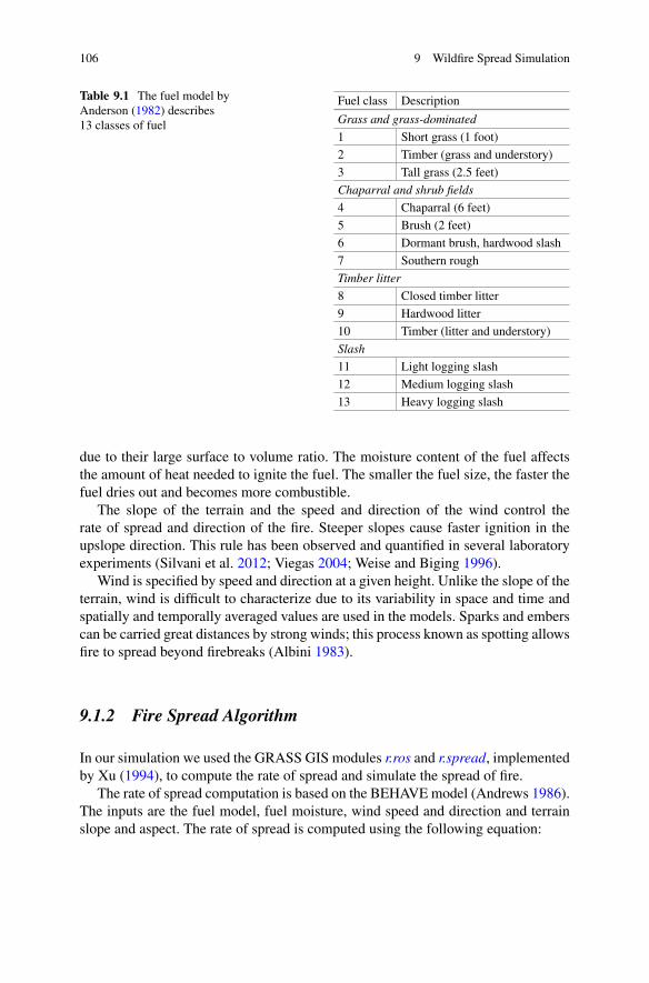
The fuel model is one of the most important input variables for fire simulation.Albini (1976) and Anderson (1982) describe 13 classes of fuel (Table 9.1), whichdiffer in fuel loads and the distribution of fuel particle size classes. The size ofindividual pieces of fuel influences the fire; heat is absorbed faster by small twigs

© The Author(s) 2015A. Petrasova et al., Tangible Modeling with Open Source GIS,DOI 10.1007/978-3-319-25775-4_9

105

106 9 Wildfire Spread Simulation

Table 9.1 The fuel model byAnderson (1982) describes13 classes of fuel

Fuel class Description

Grass and grass-dominated

1 Short grass (1 foot)

2 Timber (grass and understory)

3 Tall grass (2.5 feet)

Chaparral and shrub fields

4 Chaparral (6 feet)

5 Brush (2 feet)

6 Dormant brush, hardwood slash

7 Southern rough

Timber litter

8 Closed timber litter

9 Hardwood litter

10 Timber (litter and understory)

Slash

11 Light logging slash

12 Medium logging slash

13 Heavy logging slash

due to their large surface to volume ratio. The moisture content of the fuel affectsthe amount of heat needed to ignite the fuel. The smaller the fuel size, the faster thefuel dries out and becomes more combustible.

The slope of the terrain and the speed and direction of the wind control therate of spread and direction of the fire. Steeper slopes cause faster ignition in theupslope direction. This rule has been observed and quantified in several laboratoryexperiments (Silvani et al. 2012; Viegas 2004; Weise and Biging 1996).

Wind is specified by speed and direction at a given height. Unlike the slope of theterrain, wind is difficult to characterize due to its variability in space and time andspatially and temporally averaged values are used in the models. Sparks and emberscan be carried great distances by strong winds; this process known as spotting allowsfire to spread beyond firebreaks (Albini 1983).

9.1.2 Fire Spread Algorithm

In our simulation we used the GRASS GIS modules r.ros and r.spread, implementedby Xu (1994), to compute the rate of spread and simulate the spread of fire.

The rate of spread computation is based on the BEHAVE model (Andrews 1986).The inputs are the fuel model, fuel moisture, wind speed and direction and terrainslope and aspect. The rate of spread is computed using the following equation:

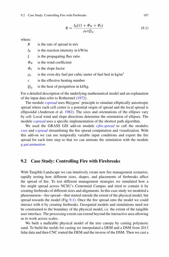
9.2 Case Study: Controlling Fire with Firebreaks 107

R D IR�.1 C ˚W C ˚S/

�b"Qig(9.1)

where:R is the rate of spread in m/s

IR is the reaction intensity in kW/m

� is the propagating flux ratio

˚W is the wind coefficient

˚S is the slope factor

�b is the oven-dry fuel per cubic meter of fuel bed in kg/m3

" is the effective heating number

Qig is the heat of preignition in kJ/kg.

For a detailed description of the underlying mathematical model and an explanationof the input data refer to Rothermel (1972).

The module r.spread uses Huygens’ principle to simulate elliptically anisotropicspread where each cell center is a potential origin of spread and the local spread isellipsoidal (Anderson et al. 1982). The sizes and orientations of the ellipses varyby cell. Local wind and slope directions determine the orientation of ellipses. Themodule r.spread uses a specific implementation of the shortest path algorithm.

We used the GRASS GIS add-on module r.fire.spread to call the modulesr.ros and r.spread streamlining the fire spread computation and visualization. Withthis add-on we can use temporally variable input conditions and export the firespread for each time step so that we can animate the simulation with the moduleg.gui.animation.

9.2 Case Study: Controlling Fire with Firebreaks

With Tangible Landscape we can intuitively create new fire management scenarios,rapidly testing how different sizes, shapes, and placements of firebreaks affectthe spread of fire. To test different management strategies we simulated how afire might spread across NCSU’s Centennial Campus and tried to contain it bycreating firebreaks of different sizes and alignments. In this case study we modeled aphenomenon—fire spread—that started outside the extent of the physical model, butspread towards the model (Fig. 9.1). Once the fire spread onto the model we couldinteract with it by creating firebreaks. Geospatial models and simulations need notbe constrained to the boundary of the physical model, i.e. the extent of the tangibleuser interface. The processing extent can extend beyond the interactive area allowingus to work across scales.

We built a malleable physical model of the tree canopy by casting polymericsand. To build the molds for casting we interpolated a DEM and a DSM from 2013lidar data and then CNC routed the DEM and the inverse of the DSM. Then we cast a

108 9 Wildfire Spread Simulation

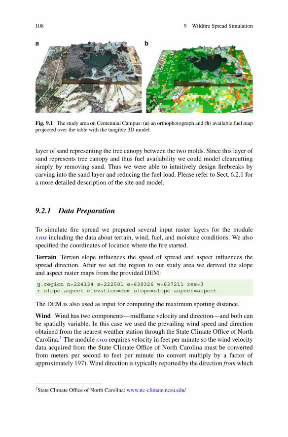
Fig. 9.1 The study area on Centennial Campus: (a) an orthophotograph and (b) available fuel mapprojected over the table with the tangible 3D model

layer of sand representing the tree canopy between the two molds. Since this layer ofsand represents tree canopy and thus fuel availability we could model clearcuttingsimply by removing sand. Thus we were able to intuitively design firebreaks bycarving into the sand layer and reducing the fuel load. Please refer to Sect. 6.2.1 fora more detailed description of the site and model.

9.2.1 Data Preparation

To simulate fire spread we prepared several input raster layers for the moduler.ros including the data about terrain, wind, fuel, and moisture conditions. We alsospecified the coordinates of location where the fire started.

Terrain Terrain slope influences the speed of spread and aspect influences thespread direction. After we set the region to our study area we derived the slopeand aspect raster maps from the provided DEM:

g.region n=224134 s=222501 e=639326 w=637211 res=3r.slope.aspect elevation=dem slope=slope aspect=aspect

The DEM is also used as input for computing the maximum spotting distance.

Wind Wind has two components—midflame velocity and direction—and both canbe spatially variable. In this case we used the prevailing wind speed and directionobtained from the nearest weather station through the State Climate Office of NorthCarolina.1 The module r.ros requires velocity in feet per minute so the wind velocitydata acquired from the State Climate Office of North Carolina must be convertedfrom meters per second to feet per minute (to convert multiply by a factor ofapproximately 197). Wind direction is typically reported by the direction from which

1State Climate Office of North Carolina: www.nc-climate.ncsu.edu/

9.2 Case Study: Controlling Fire with Firebreaks 109

it originates, clockwise from the north. The module r.ros, however, requires the “to”direction (also clockwise from north). To simulate spatial variability we applied arandom effect, for example, using the module r.surf.gauss to produce a raster mapof Gaussian deviates with a specified mean and standard deviation:

r.surf.gauss output=wind_speed_avg mean=542 sigma=30r.surf.gauss output=wind_dir mean=75 sigma=20

Fuel The module r.ros uses Anderson’s 13 standard fire behavior fuel models.Fuel data layers at 30 m resolution for the USA are publicly accessible via theLANDFIRE website.2 Most of our study site falls into fuel classes 8 and 9, i.e.timber litter (Fig. 9.1b).

Moisture Since fuel moisture data were not readily available for our site wegenerated the required, spatially variable raster maps of 1-h fuel moisture and livefuel moisture percentage for dry conditions:

r.surf.gauss output=moisture_1h mean=10 sigma=5r.surf.gauss output=moisture_live mean=20 sigma=5

Starting Location The starting sources of the fire are represented as raster cellsand can be created by digitizing points or importing coordinates from a file andconverting them to a raster. We provided the fire starting location in a text file withthe point coordinates (for example 638097,222934) and converted them to araster with the module v.to.rast:

v.in.ascii input=source.txt output=source separator=commav.to.rast input=source output=source type=point use=cat

9.2.2 Scenario with Multiple Firebreaks

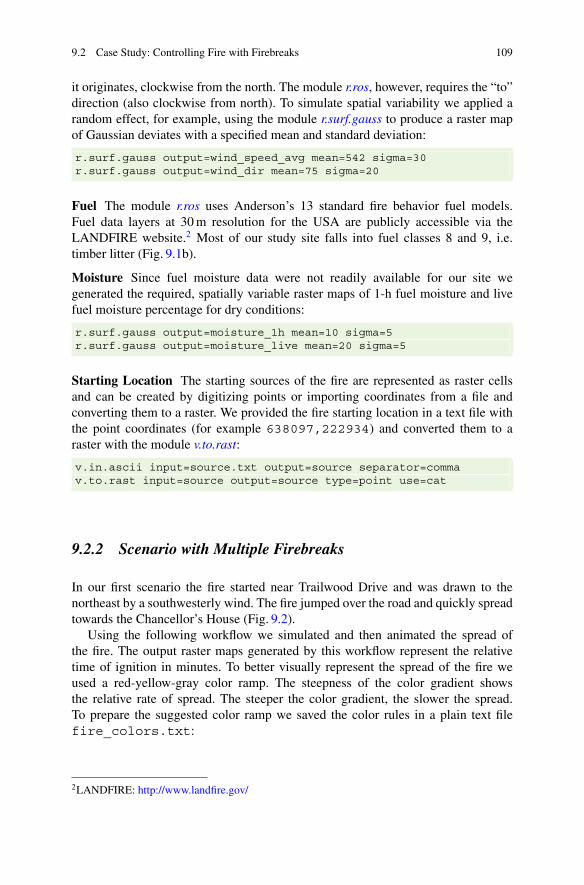
In our first scenario the fire started near Trailwood Drive and was drawn to thenortheast by a southwesterly wind. The fire jumped over the road and quickly spreadtowards the Chancellor’s House (Fig. 9.2).

Using the following workflow we simulated and then animated the spread ofthe fire. The output raster maps generated by this workflow represent the relativetime of ignition in minutes. To better visually represent the spread of the fire weused a red-yellow-gray color ramp. The steepness of the color gradient showsthe relative rate of spread. The steeper the color gradient, the slower the spread.To prepare the suggested color ramp we saved the color rules in a plain text filefire_colors.txt:

2LANDFIRE: http://www.landfire.gov/

110 9 Wildfire Spread Simulation

Fig. 9.2 The spread of the fire without intervention

0% 50:50:5060% yellow100% red

To run the simulation we called the module r.ros once and then r.spread with thedesired time lag parameter specifying the length of the simulation. To see theintermediate states we can run the module r.spread multiple times and assign ourcolor ramp to the resulting spread raster map:

r.ros model=fuel moisture_1h=moisture_1h \moisture_live=moisture_live velocity=wind_speed_avg \direction=wind_dir slope=slope aspect=aspect \elevation=elevation base_ros=out_base_ros \max_ros=out_max_ros direction_ros=out_dir_ros \spotting_distance=out_spotting

r.spread -s base_ros=out_dir_ros max_ros=out_max_ros \direction_ros=out_dir_ros start=source \spotting_distance=out_spotting wind_speed=wind_speed_avg \fuel_moisture=moisture_1h output=spread_1 lag=20

r.spread -s -i base_ros=out_dir_ros max_ros=out_max_ros \direction_ros=out_dir_ros start=spread_1 \spotting_distance=out_spotting wind_speed=wind_speed_avg \fuel_moisture=moisture_1h output=spread_2 lag=20

r.spread ...

9.2 Case Study: Controlling Fire with Firebreaks 111

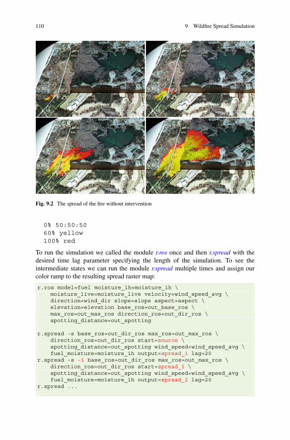
Fig. 9.3 Creating a firebreak by (a) manually removing sand and then (b) scanning and detectingthe change

r.null map=spread_1 setnull=0r.colors map=spread_1 rules=fire_colors.txt

Alternatively we can use the add-on module r.fire.spread, which conveniently wrapsthe previous sequence of commands into a single command:

r.fire.spread -s start=source times=0 end_time=1600 \time_step=20 output=spread model=fuel \moisture_1h=moisture_1h moisture_live=moisture_live \direction=wind_dir slope=slope aspect=aspect \elevation=elevation speed=wind_speed_avg

After simulating the initial spread of the fire we attempted to prevent fire fromspreading towards Chancellor’s House by creating firebreaks. First we scanned themodel to save the unmodified state. Next we manually removed sand (representingcanopy) from the location where we want to have a firebreak (see Fig. 9.3a).We scanned the modified model and vertically matched the new scan to theunmodified scan using the function defined in code snippet 4.2.2. We derived thenew fuel raster layer based on the difference between the two scans introducing nodata values into the copy of the original fuel model using a simple raster algebraexpression:

adjust_scan(’scan_before’, ’scan_after’, ’scan_adjusted’)gscript.mapcalc("changed_fuel = if(scan_before - scan_adjusted

> 0, null(), fuel)")

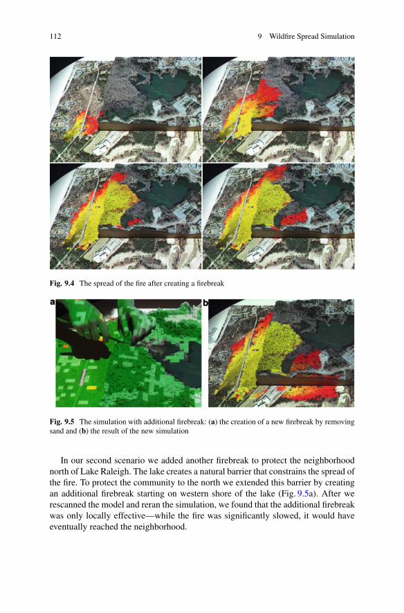
We repeated our simulation using the new fuel raster layer. The resultingfire spread in Fig. 9.4 shows that our attempt was only a partial success. Whilewe significantly slowed the spread of the fire, potentially giving firefighters moretime to act, the fire jumped over the firebreak and started to spread towardsChancellor’s House suggesting that a wider firebreak would be needed. With moreprecise data about fire behavior we could control and limit the spotting effect in thesimulation.

112 9 Wildfire Spread Simulation

Fig. 9.4 The spread of the fire after creating a firebreak

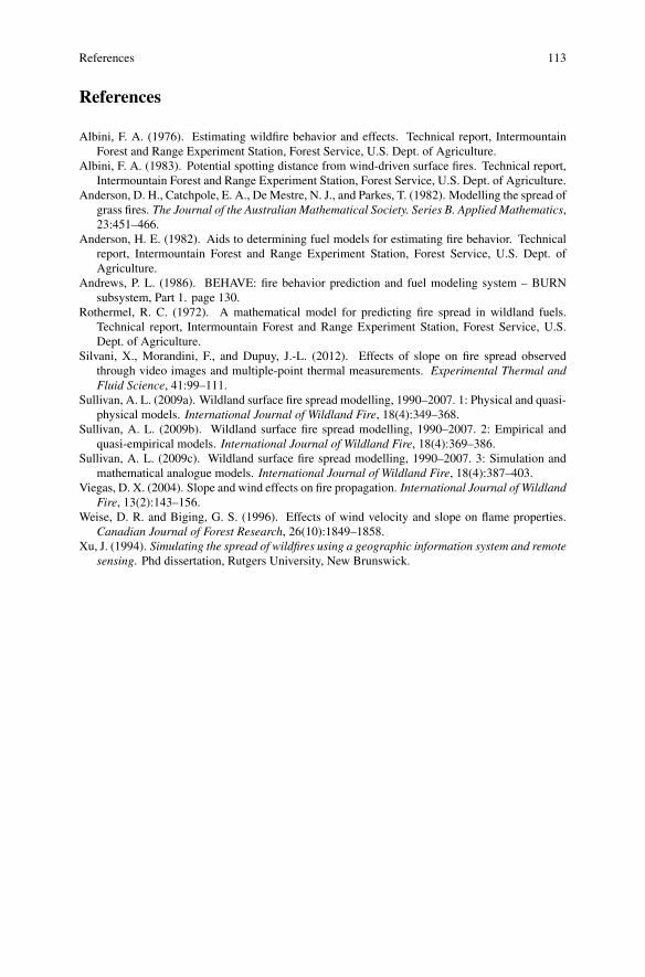
Fig. 9.5 The simulation with additional firebreak: (a) the creation of a new firebreak by removingsand and (b) the result of the new simulation

In our second scenario we added another firebreak to protect the neighborhoodnorth of Lake Raleigh. The lake creates a natural barrier that constrains the spread ofthe fire. To protect the community to the north we extended this barrier by creatingan additional firebreak starting on western shore of the lake (Fig. 9.5a). After werescanned the model and reran the simulation, we found that the additional firebreakwas only locally effective—while the fire was significantly slowed, it would haveeventually reached the neighborhood.

References 113

References

Albini, F. A. (1976). Estimating wildfire behavior and effects. Technical report, IntermountainForest and Range Experiment Station, Forest Service, U.S. Dept. of Agriculture.

Albini, F. A. (1983). Potential spotting distance from wind-driven surface fires. Technical report,Intermountain Forest and Range Experiment Station, Forest Service, U.S. Dept. of Agriculture.

Anderson, D. H., Catchpole, E. A., De Mestre, N. J., and Parkes, T. (1982). Modelling the spread ofgrass fires. The Journal of the Australian Mathematical Society. Series B. Applied Mathematics,23:451–466.

Anderson, H. E. (1982). Aids to determining fuel models for estimating fire behavior. Technicalreport, Intermountain Forest and Range Experiment Station, Forest Service, U.S. Dept. ofAgriculture.

Andrews, P. L. (1986). BEHAVE: fire behavior prediction and fuel modeling system – BURNsubsystem, Part 1. page 130.

Rothermel, R. C. (1972). A mathematical model for predicting fire spread in wildland fuels.Technical report, Intermountain Forest and Range Experiment Station, Forest Service, U.S.Dept. of Agriculture.

Silvani, X., Morandini, F., and Dupuy, J.-L. (2012). Effects of slope on fire spread observedthrough video images and multiple-point thermal measurements. Experimental Thermal andFluid Science, 41:99–111.

Sullivan, A. L. (2009a). Wildland surface fire spread modelling, 1990–2007. 1: Physical and quasi-physical models. International Journal of Wildland Fire, 18(4):349–368.

Sullivan, A. L. (2009b). Wildland surface fire spread modelling, 1990–2007. 2: Empirical andquasi-empirical models. International Journal of Wildland Fire, 18(4):369–386.

Sullivan, A. L. (2009c). Wildland surface fire spread modelling, 1990–2007. 3: Simulation andmathematical analogue models. International Journal of Wildland Fire, 18(4):387–403.

Viegas, D. X. (2004). Slope and wind effects on fire propagation. International Journal of WildlandFire, 13(2):143–156.

Weise, D. R. and Biging, G. S. (1996). Effects of wind velocity and slope on flame properties.Canadian Journal of Forest Research, 26(10):1849–1858.

Xu, J. (1994). Simulating the spread of wildfires using a geographic information system and remotesensing. Phd dissertation, Rutgers University, New Brunswick.