Embed Size (px)
Citation preview
Chapter 6
Estimates and Sample Sizes

Lesson 6-1/6-2, Part 1
Estimating a Population Proportion
This chapter begins the beginning of inferential statistics.
1. Estimate the value of a population
parameter (proportions, means and
variances).
2. Test some claim (or hypothesis) about a
population.
There are two major applications of inferential
statistics involve the use of sample data to:
Overview
Introduce methods for estimating values of these important population parameters: proportions, means, and variances.
Present methods for determining samples sizes necessary to estimate those parameters.
Assumptions
Randomization condition – Were the data sampled at random or generated from a properly randomization experiment?
10% Condition (N ≥ 10n) – Samples are almost always drawn without replacement. If the sample exceeds 10% of the population, the probability of a success changes so much during the sampling that our Normal model may no longer be appropriate.
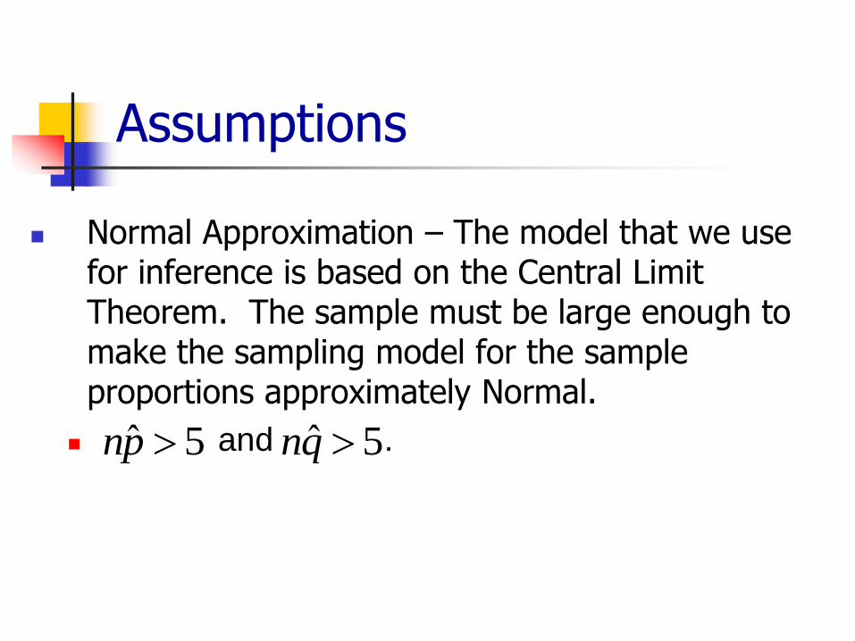
Assumptions
Normal Approximation – The model that we use for inference is based on the Central Limit Theorem. The sample must be large enough to make the sampling model for the sample proportions approximately Normal.
and .ˆ 5np ˆ 5nq
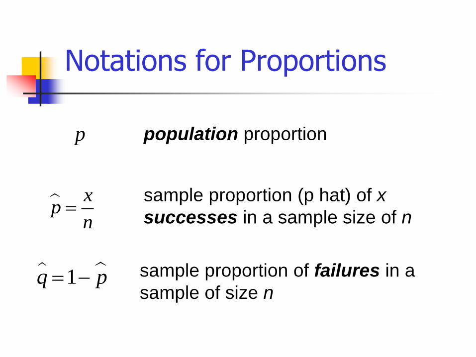
Notations for Proportions
xp
n
sample proportion (p hat) of x
successes in a sample size of n
1q p sample proportion of failures in a
sample of size n
population proportionp
Point Estimate
A point estimate is a single value (or point) used to approximate a population parameter.
The sample proportion is the best point estimate of the population proportion .
p̂ p
Confidence Interval or Interval Estimate
A confidence interval (or interval estimate) is a range (or an interval) of values used to estimate the true value of a population parameter.
A confidence interval is sometimes abbreviated as CI.
Confidence Interval
A confidence level is the probability 1 – α (often
expressed as the equivalent percentage value) that
is the proportion of times that confidence interval
actually does contain the population parameter,
assuming that the estimate process is repeated a
large number of times.
This is usually 90% (α = 10%), 95% (α = 5%) or 99%
(α = 1%)
The confidence level is also called the degree of
confidence, or the confidence coefficient.
Interpreting the Confidence Level
The statement “95% confident” means in repeated sampling, 95 percent of the intervals produced using this method will contain the proportion of adult Minnesotans who would respond no to the question “photo cop legislation.”
If 1000 samples of size 829 were taken about 1000(0.95) = 950 of the intervals would contain the parameter p and about 50 would not.
What can we really say about p?
“51 % of all Minnesotans are opposed to photo-cop legislations.” It would be nice to be able to make absolute statements
about population values with certainty, but we just don’t have enough information do that.
There’s no way to be sure that the population proportion is the same as the sample proportion; in fact, it almost certainly isn’t. Observations vary. Another sample would yield a different sample proportion.
What can we really say about p?
“It is probably true that 51 % of all Minnesotans are opposed to photo-cop legislations.” No. In fact we can be pretty sure that whatever the true
proportion is, it’s not exactly 51%. So the statement is not true.
What can we really say about p?
“We don’t know exactly what proportion of Minnesotans are opposed to photo-cop legislations but we know that it’s between the interval from 48% and 54%.”
This it getting closer, but we still can’t certain. We can’t know for sure that the true proportion is in this range – or any particular range.
What can we really say about p?
“We don’t know exactly what proportion of Minnesotans are opposed to photo-cop legislations but interval from 48% and 54% probably contains the true value.”
We’ve now fudge twice – first by giving an interval and second by admitting that we only think the interval “probably” contains the true value. This statement is true.
What can we really say about p?
The last statement may be true, but it’s a bit wishy-washy. We can tighten it up bit quantifying what we meant by “probably”.
We are 95% confident that between 48% and 54% of Minnesotans opposed photo-cop legislation.
Critical Value
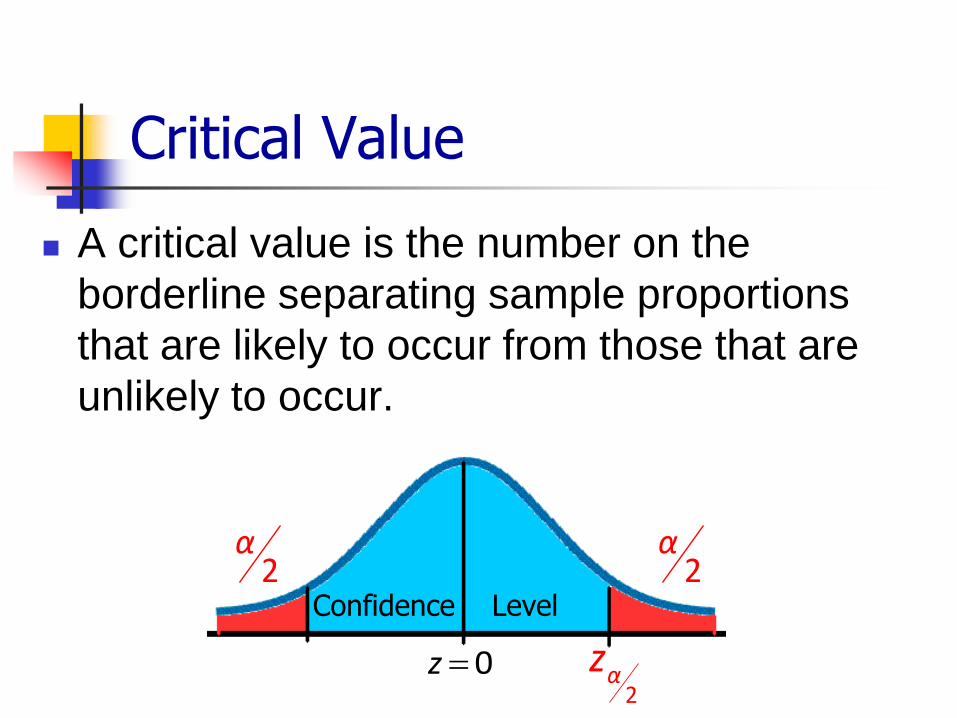
A critical value is the number on the
borderline separating sample proportions
that are likely to occur from those that are
unlikely to occur.
2α
2α
0z 2
αz
Confidence Level
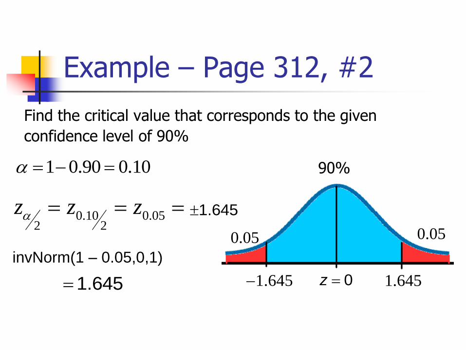
Example – Page 312, #2
Find the critical value that corresponds to the given
confidence level of 90%
1 0.90 0.10
0.10 0.052 2
z z z
1.645 1.645
0.050.05
invNorm(1 – 0.05,0,1)
90%
z 01.645
1.645
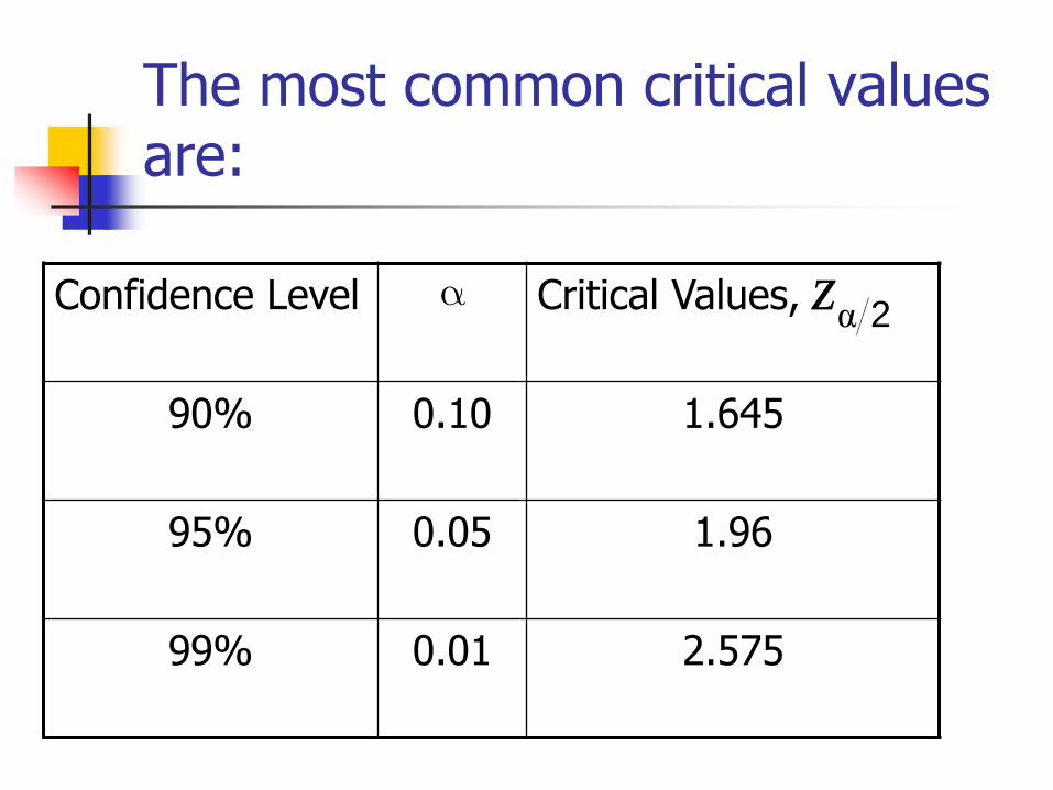
The most common critical values are:
Confidence Level Critical Values,
90% 0.10 1.645
95% 0.05 1.96
99% 0.01 2.575
α 2z
Margin of Error
When data from a simple random sample are used to estimate a population proportion p, the margin of error, denoted by E, is the maximum likely (with probability 1 – α) difference
between the observed proportion
and the true value of the population
proportion p.
p̂
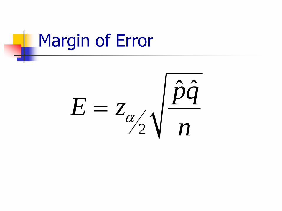
Margin of Error
2
ˆ ˆ
pqE z
n
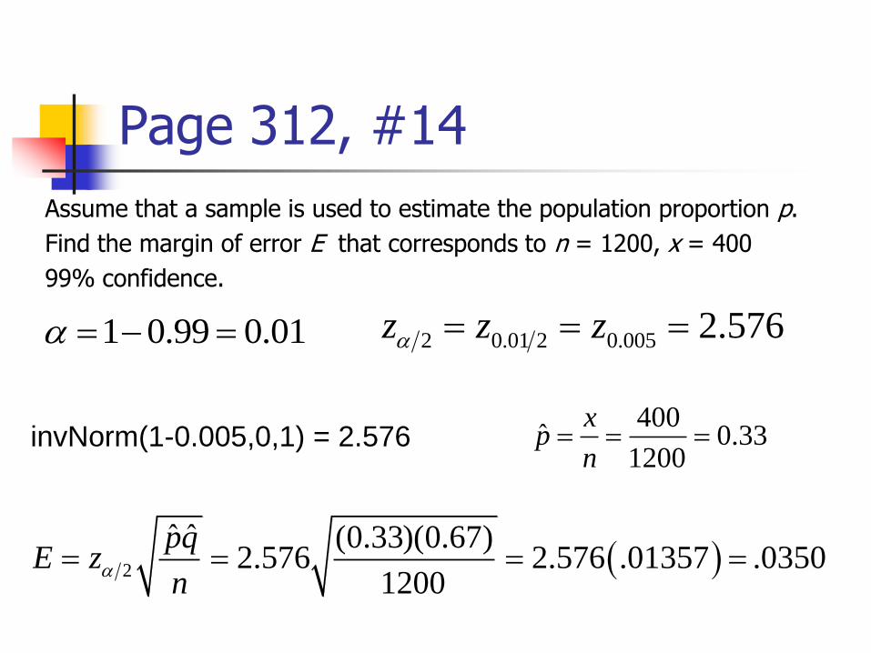
Page 312, #14
Assume that a sample is used to estimate the population proportion p.
Find the margin of error E that corresponds to n = 1200, x = 400
99% confidence.
1 0.99 0.01
400ˆ 0.33
1200
xp
n
2
ˆ ˆ (0.33)(0.67)2.576 2.576 .01357 .0350
1200
pqE z
n
2 0.01 2 0.005 2.576 z z z
invNorm(1-0.005,0,1) = 2.576
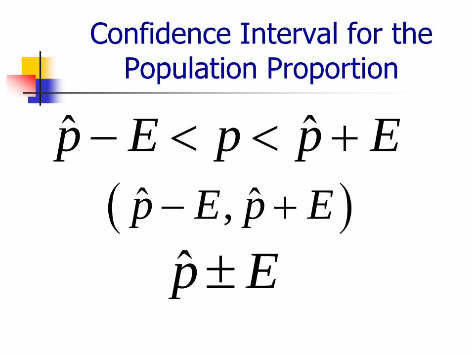
Confidence Interval for thePopulation Proportion
ˆ ˆ p E p p E
ˆ p E
ˆ ˆ, p E p E
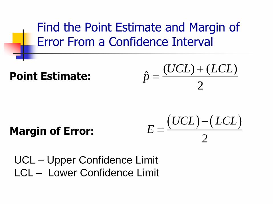
Find the Point Estimate and Margin of Error From a Confidence Interval
( ) ( )ˆ
2
UCL LCLp
2
UCL LCLE
UCL – Upper Confidence Limit
LCL – Lower Confidence Limit
Point Estimate:
Margin of Error:
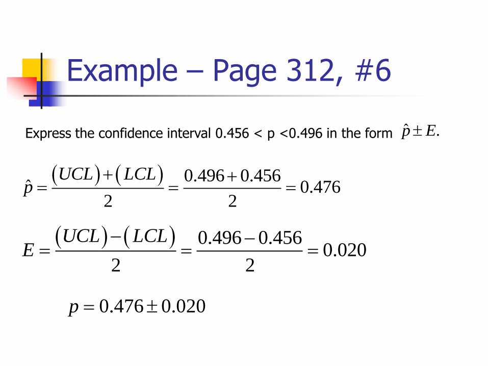
Example – Page 312, #6
ˆ .p E
0.496 0.456ˆ 0.476
2 2
UCL LCLp
0.496 0.4560.020
2 2
UCL LCLE
0.476 0.020p
Express the confidence interval 0.456 < p <0.496 in the form
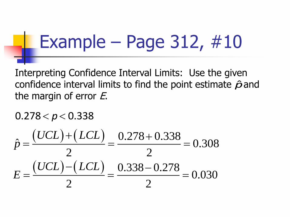
Example – Page 312, #10
Interpreting Confidence Interval Limits: Use the given confidence interval limits to find the point estimate andthe margin of error E.
p̂
0.278 0.338p
0.278 0.338ˆ 0.308
2 2
UCL LCLp
0.338 0.2780.030
2 2
UCL LCLE
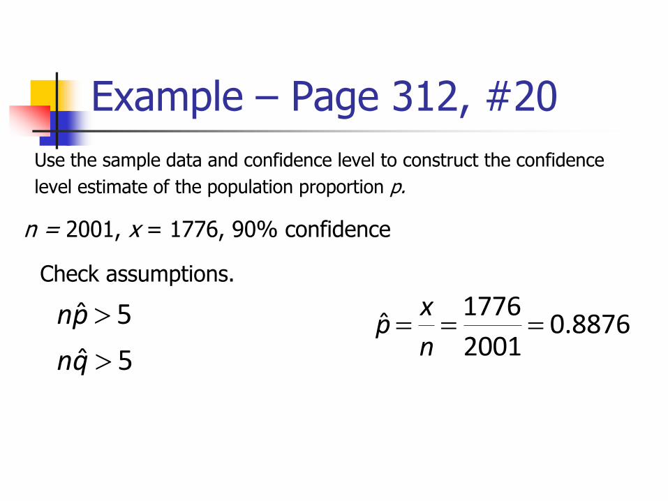
Example – Page 312, #20
Use the sample data and confidence level to construct the confidence
level estimate of the population proportion p.
n = 2001, x = 1776, 90% confidence
Check assumptions.
ˆ 5
ˆ 5
np
nq
1776ˆ 0.8876
2001
xp
n
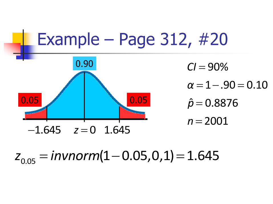
Example – Page 312, #20
90%
1 .90 0.10
ˆ 0.8876
2001
CI
α
p
n
0.90
0.050.05
0z
0.05 (1 0.05,0,1) 1.645z invnorm
1.645 1.645
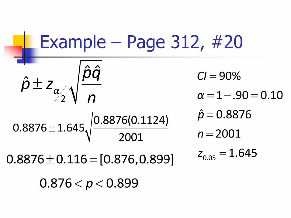
Example – Page 312, #20
0.05
90%
1 .90 0.10
ˆ 0.8876
2001
1.645
CI
α
p
n
z
2
ˆ ˆˆ α
pqp z
n
0.8876(0.1124)0.8876 1.645
2001
0.8876 0.116 [0.876,0.899]
0.876 0.899p
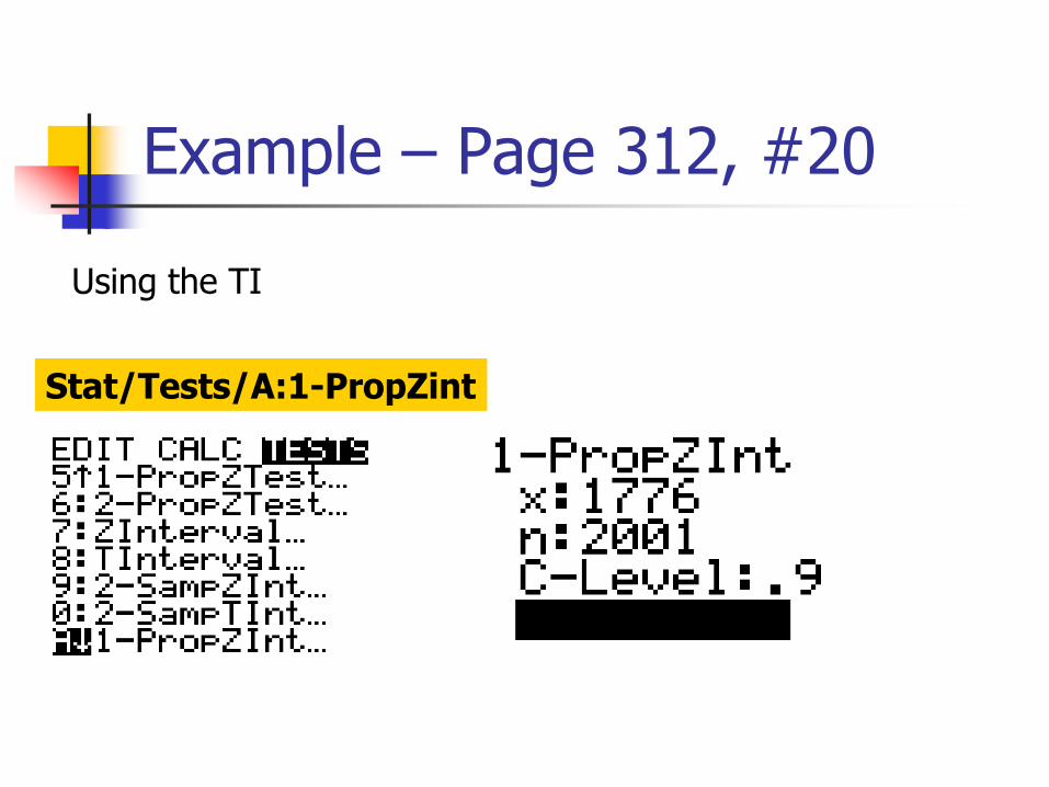
Example – Page 312, #20
Stat/Tests/A:1-PropZint
Using the TI
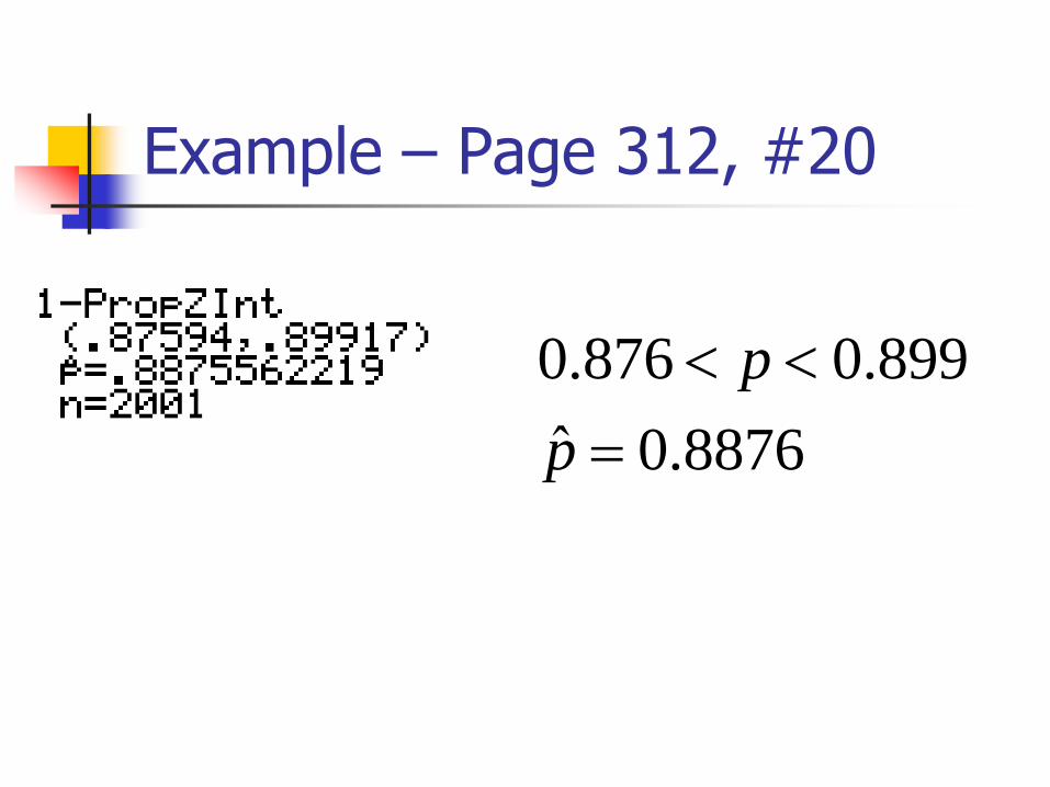
Example – Page 312, #20
0.876 0.899
ˆ 0.8876
p
p
Lesson 6-1/6-2, Part 2
Estimating a Population Proportion
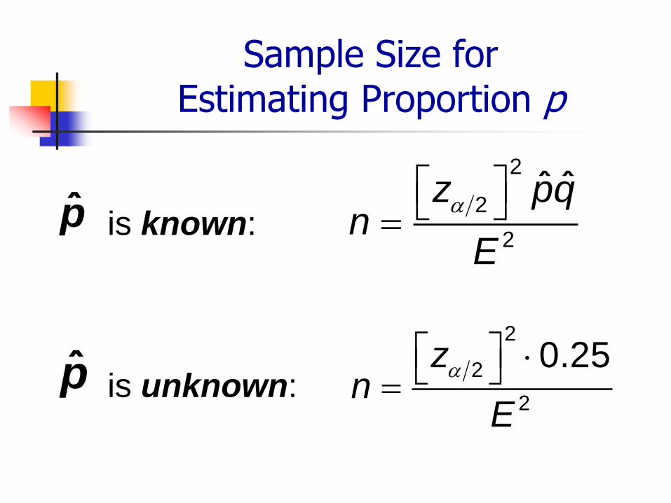
Sample Size for Estimating Proportion p
is known:p̂
2
2
2
ˆ ˆz pq
nE
p̂ is unknown:z
nE
2
2
2
0.25
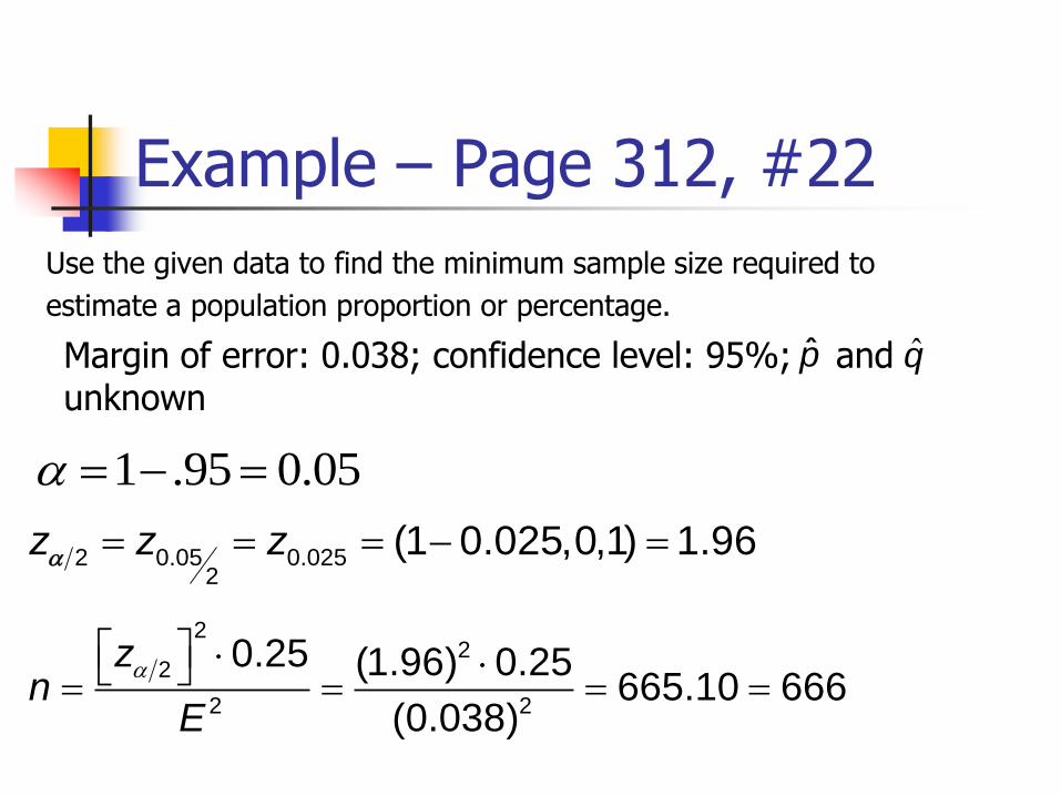
Example – Page 312, #22
Use the given data to find the minimum sample size required to
estimate a population proportion or percentage.
p̂
zn
E
22
2
2 2
0.25 (1.96) 0.25665.10 666
(0.038)
q̂
1 .95 0.05
2 0.05 0.0252
(1 0.025,0,1) 1.96z z z
Margin of error: 0.038; confidence level: 95%; and unknown
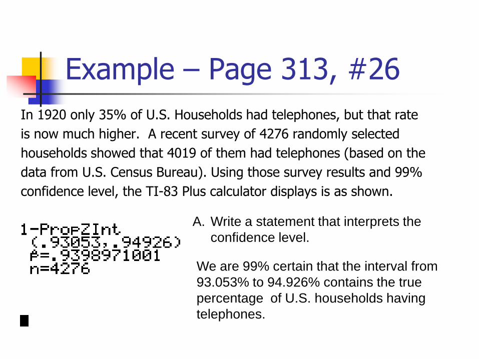
Example – Page 313, #26
In 1920 only 35% of U.S. Households had telephones, but that rate
is now much higher. A recent survey of 4276 randomly selected
households showed that 4019 of them had telephones (based on the
data from U.S. Census Bureau). Using those survey results and 99%
confidence level, the TI-83 Plus calculator displays is as shown.
A. Write a statement that interprets the
confidence level.
We are 99% certain that the interval from
93.053% to 94.926% contains the true
percentage of U.S. households having
telephones.
Example – Page 313, #26
B. Based on the preceding results, should pollsters be concerned about results from surveys conducted by phone.
Yes. Based on the results from part (a), about 5% to 7%of the population does not have telephone, so those people are missed.
Procedure for Constructing a Confidence Interval for p
Identify the population of interest and the parameter you want to draw conclusions about.
Choose the appropriate inference procedure. Verify the conditions for using the selected procedure.
If the conditions are met, carry out the inference.
Interpret your results in the context of the problem.
Example – Page 313, #28
Death Penalty Survey: In a Gallup Poll, 491 randomly selected adults
were asked whether they are in favor of the death penalty for a person
convicted of murder, and 65% of them said that they were in favor.
A. Find the point estimate of the percentage of adults
who are in favor of this death penalty.
65% is the point estimate
Example – Page 313, #28
B. Find a 95% confidence interval estimate of the percentage of adults who are in favor of this death penalty.
p = proportion of adults who are in favor of the death penalty for a person convicted of murder
Step 1 – Identify the population of interest and parameter you want to draw conclusion about.
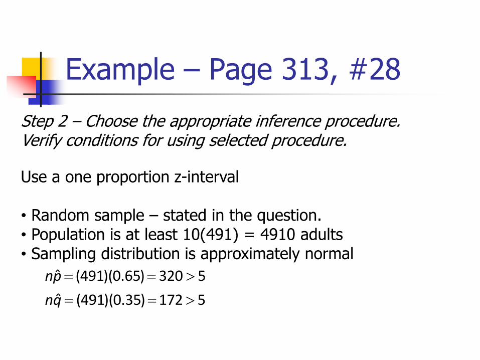
Example – Page 313, #28
Step 2 – Choose the appropriate inference procedure. Verify conditions for using selected procedure.
Use a one proportion z-interval
• Random sample – stated in the question.• Population is at least 10(491) = 4910 adults• Sampling distribution is approximately normal
ˆ (491)(0.65) 320 5
ˆ (491)(0.35) 172 5
np
nq
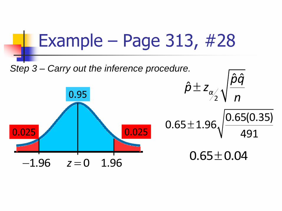
Example – Page 313, #28
0.95
0.0250.025
0z 1.96 1.96
Step 3 – Carry out the inference procedure.
2
ˆ ˆˆ α
pqp z
n
0.65(0.35)0.65 1.96
491
0.65 0.04
Example – Page 313, #28
We 95% confident that the proportion of adults who are in favor of the death penalty for a person convicted of murderis between 61% and 69%.
Step 4 – Interpret you results in the context of the problem.
Example – Page 313, #28
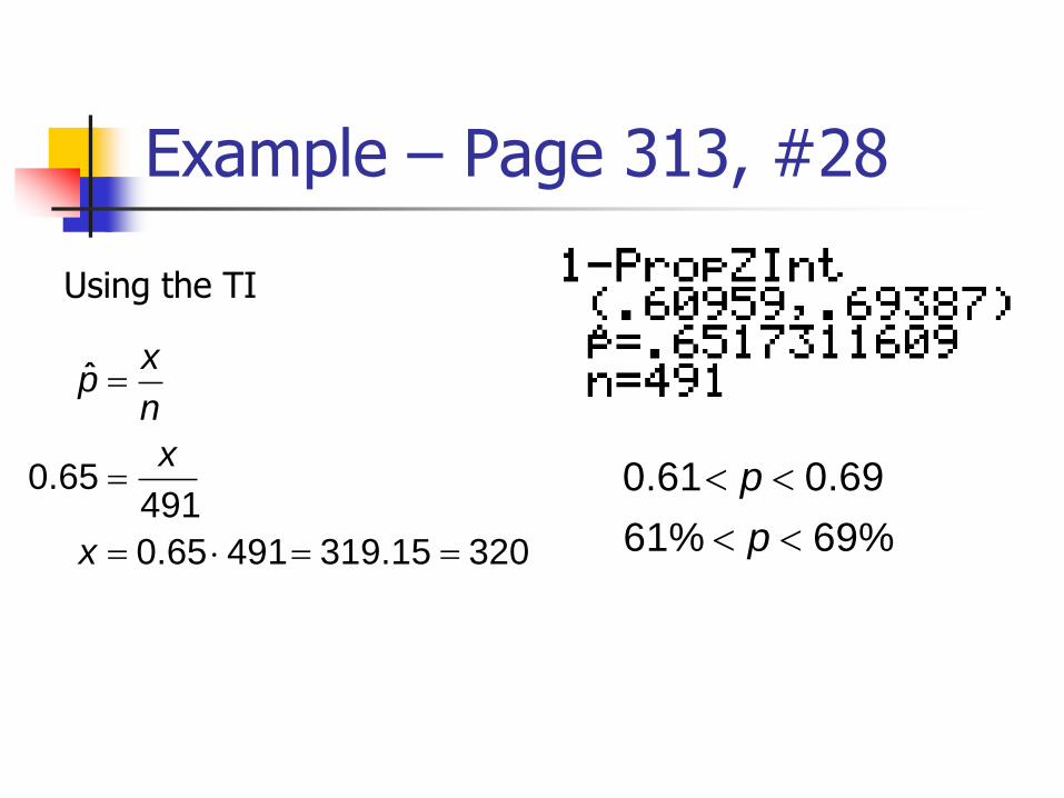
ˆ
0.65491
0.65 491 319.15 320
xp
n
x
x
p
p
0.61 0.69
61% 69%
Using the TI
C. Can we safely conclude that the majority of adults are
in favor of this death penalty? Explain
Example – Page 313, #28
Yes, since the interval in which we have 95%
confidence is entirely above 50%
Example – Page 314, #34
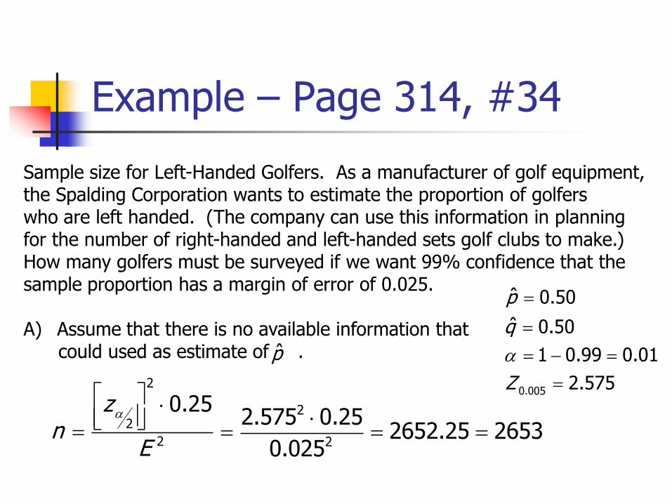
Sample size for Left-Handed Golfers. As a manufacturer of golf equipment,the Spalding Corporation wants to estimate the proportion of golferswho are left handed. (The company can use this information in planningfor the number of right-handed and left-handed sets golf clubs to make.)How many golfers must be surveyed if we want 99% confidence that thesample proportion has a margin of error of 0.025.
A) Assume that there is no available information that could used as estimate of .p̂
2
2
2
0.25zn
E
2
2
2.575 0.252652.25 2653
0.025
0.005
ˆ 0.50
ˆ 0.50
1 0.99 0.01
2.575
p
q
Z
Example – Page 314, #34
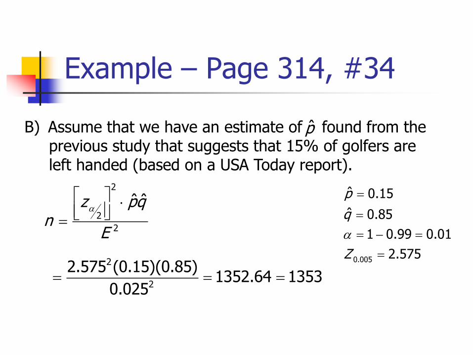
B) Assume that we have an estimate of found from the previous study that suggests that 15% of golfers areleft handed (based on a USA Today report).
p̂
2
2
2
ˆˆz pqn
E
2
2
2.575 (0.15)(0.85)1352.64 1353
0.025
0.005
ˆ 0.15
ˆ 0.85
1 0.99 0.01
2.575
p
q
Z
Example – Page 314, #34
C) Assume that instead of using randomly selected golfers, thesample data are obtained by asking TV viewers of the golfingchannel to call an “800” phone number to report whetherthey are left-handed or right-handed. How are the resultsaffected?
Self selected samples are not valid. It is not appropriateto assume that those who respond will be representative ofthe general population.
Lesson 6-3
Estimating a Population Mean: σ Known
Assumptions
Sample is a simple random sample
Values of the population standard deviation σ is known
The population is normally distributed or n >30.
Example – Page 327, #6
Verify the assumptions. Determine whether the givenconditions justify using the margin of error when findinga confidence interval estimate of the population mean μ
The sample size is n = 5 and σ not known.
No, n is not greater than 30 and standard deviation is not known.
Example – Page 327, #8
Verify the assumptions. Determine whether the givenconditions justify using the margin of error when findinga confidence interval estimate of the population mean μ
The sample size is n = 9, σ not known and the originalpopulation is normally distributed.
No, because σ not known.
Definitions
Estimator is a formula or process for using sample data to estimate a population parameter.
Estimate is a specific value or range of values used to approximate a population parameter.
Point Estimate is a single value (or point) used to approximate a population parameter.
The sample mean is the best point estimate of the population mean μ.
x
Confidence Interval
As we saw in Section 6-2, a confidence interval is a range (or an interval) of values used to estimate the true value of the population parameter.
The confidence level gives us the success rate of the procedure used to construct the confidence interval.
Level of Confidence
As describe in Section 6-2, The confidence level is often expressed as the probability 1 – α, where α is the complement of the
confidence level.
For a 0.95 (95%) confidence level, α = 0.05
For a 0.99 (99%) confidence level, α = 0.01
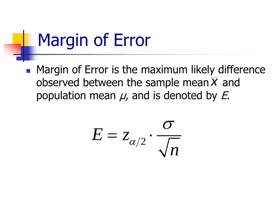
Margin of Error
Margin of Error is the maximum likely difference observed between the sample mean and population mean μ, and is denoted by E.
2
E z
n
x
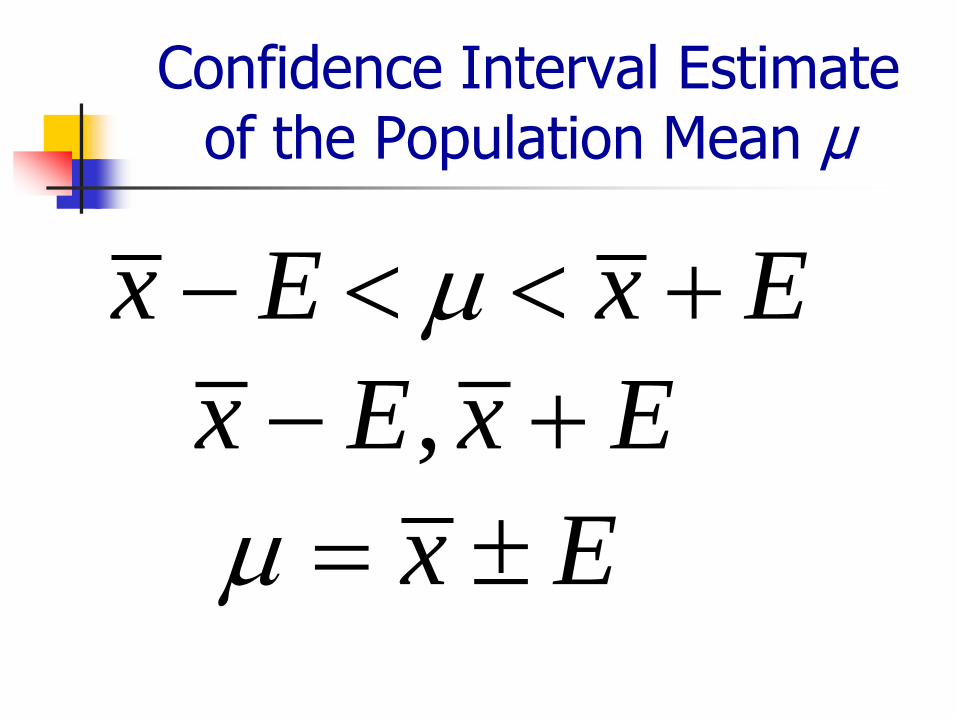
Confidence Interval Estimate of the Population Mean μ
x E x E
x E
, x E x E
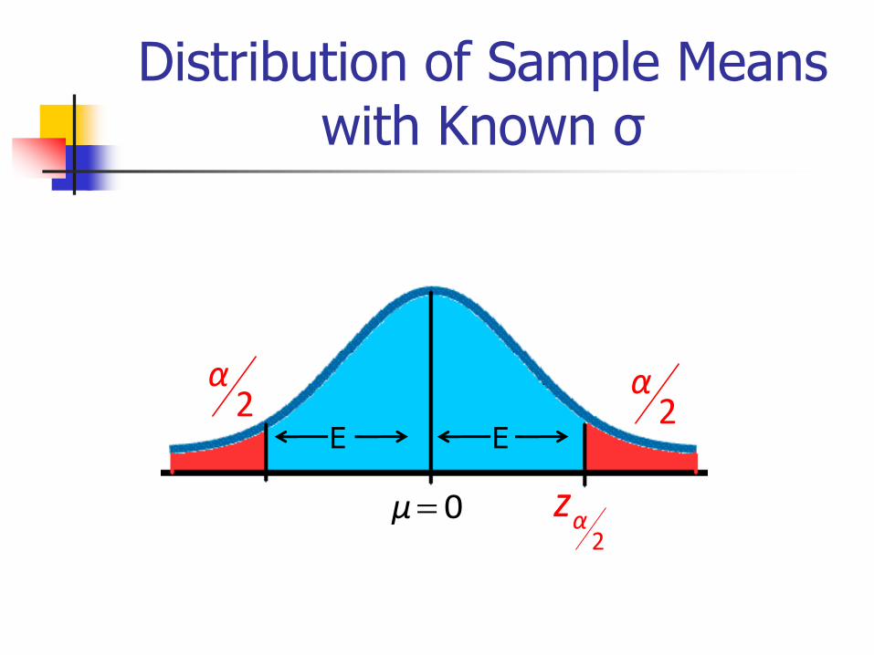
Distribution of Sample Means with Known σ
2α
2α
0μ2
αz
E E
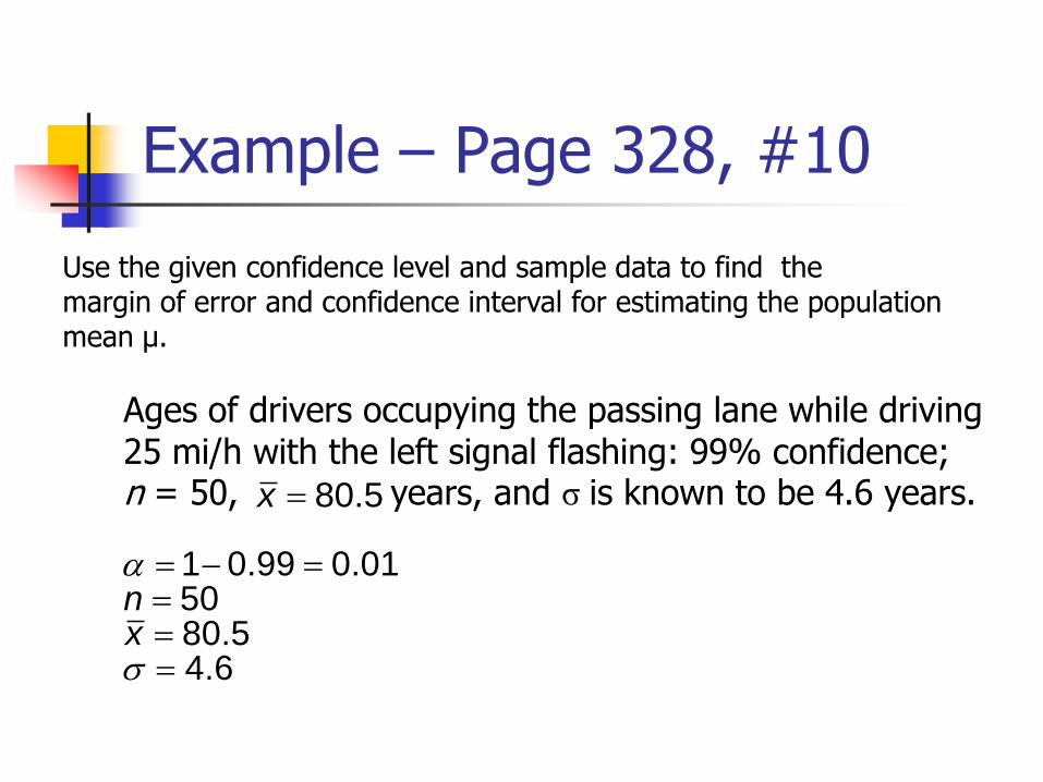
Example – Page 328, #10
Use the given confidence level and sample data to find the margin of error and confidence interval for estimating the populationmean μ.
Ages of drivers occupying the passing lane while driving25 mi/h with the left signal flashing: 99% confidence;n = 50, years, and σ is known to be 4.6 years.80.5x
1 0.99 0.015080.54.6
nx
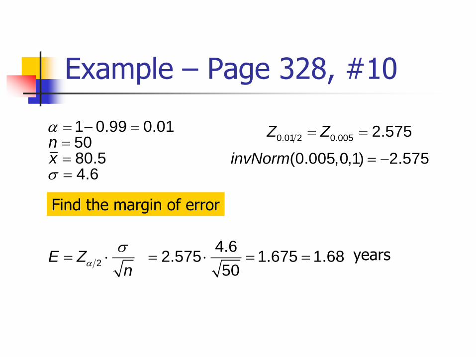
Example – Page 328, #10
1 0.99 0.015080.54.6
nx
Find the margin of error
2E Zn
0.01 2 0.005 2.575Z Z
(0.005,0,1) 2.575invNorm
4.62.575 1.675 1.68
50 years
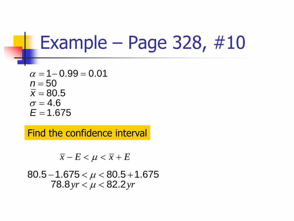
Example – Page 328, #10
1 0.99 0.015080.54.61.675
nx
E
Find the confidence interval
x E x E
80.5 1.675 80.5 1.67578.8 82.2
yr yr
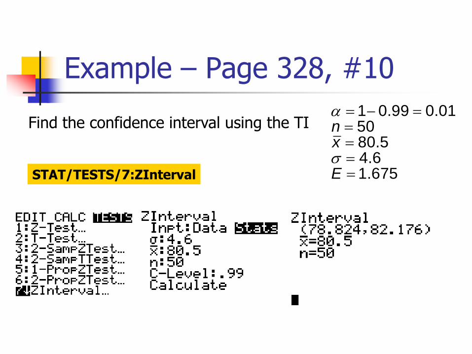
Example – Page 328, #10
1 0.99 0.015080.54.61.675
nx
E
Find the confidence interval using the TI
STAT/TESTS/7:ZInterval
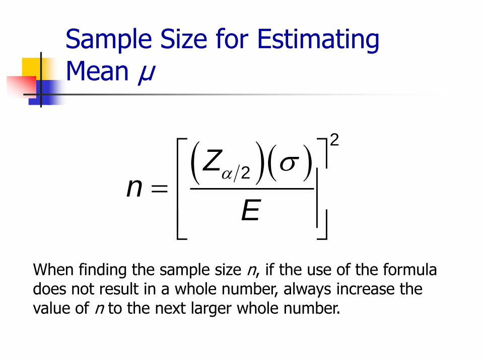
Sample Size for Estimating Mean μ
2
2Zn
E
When finding the sample size n, if the use of the formuladoes not result in a whole number, always increase thevalue of n to the next larger whole number.
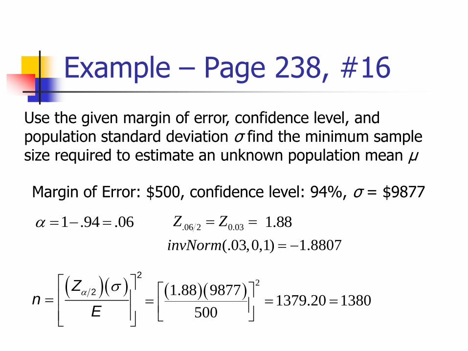
Example – Page 238, #16
Use the given margin of error, confidence level, and population standard deviation σ find the minimum samplesize required to estimate an unknown population mean μ
Margin of Error: $500, confidence level: 94%, σ = $9877
1 .94 .06 .06 2 0.03Z Z 1.88
(.03,0,1) 1.8807 invNorm
2
2Zn
E
2
1.88 98771379.20 1380
500
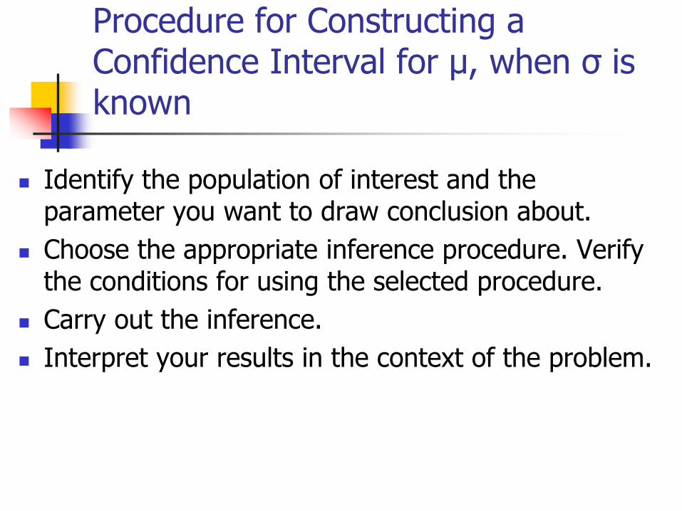
Procedure for Constructing a Confidence Interval for μ, when σ is known
Identify the population of interest and the parameter you want to draw conclusion about.
Choose the appropriate inference procedure. Verify the conditions for using the selected procedure.
Carry out the inference.
Interpret your results in the context of the problem.
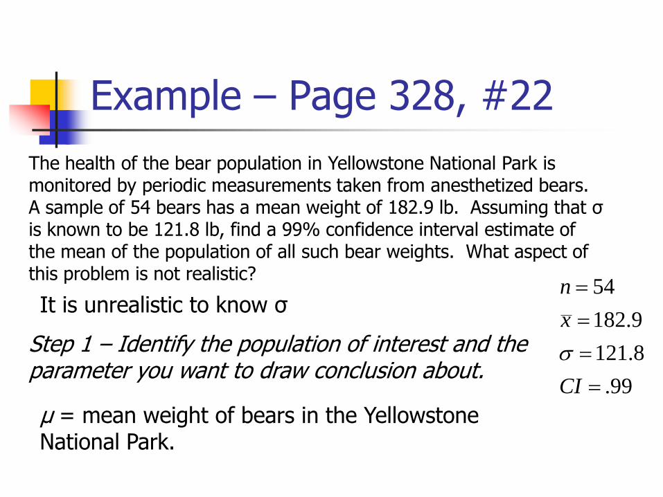
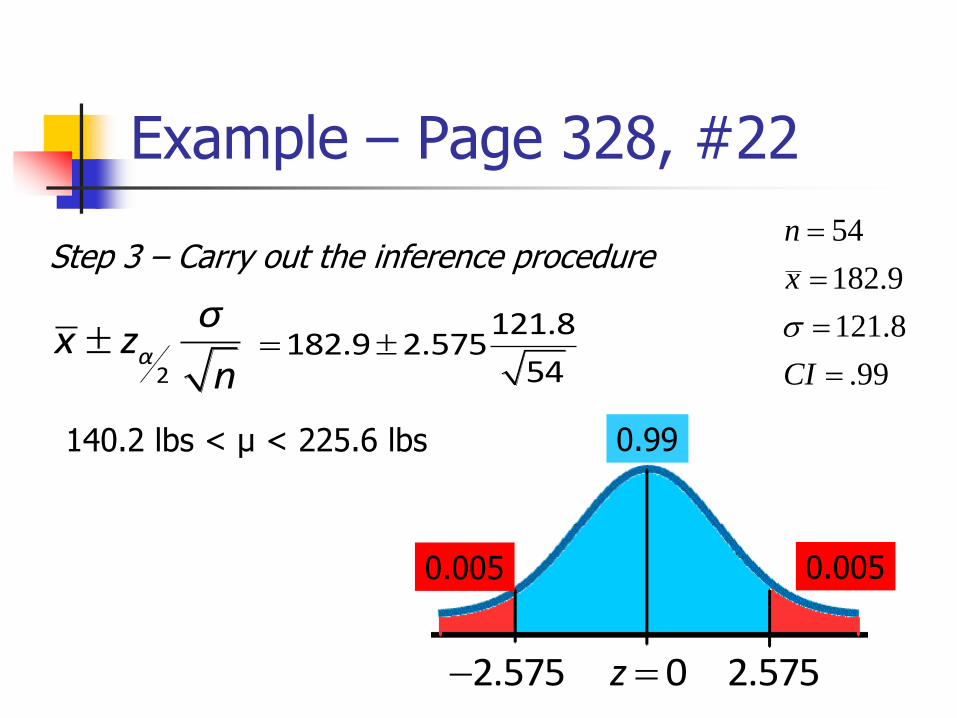
Example – Page 328, #22
The health of the bear population in Yellowstone National Park is monitored by periodic measurements taken from anesthetized bears.A sample of 54 bears has a mean weight of 182.9 lb. Assuming that σis known to be 121.8 lb, find a 99% confidence interval estimate ofthe mean of the population of all such bear weights. What aspect of this problem is not realistic?
54
182.9
121.8
.99
n
x
CI
µ = mean weight of bears in the YellowstoneNational Park.
It is unrealistic to know σ
Step 1 – Identify the population of interest and the parameter you want to draw conclusion about.
Example – Page 328, #22
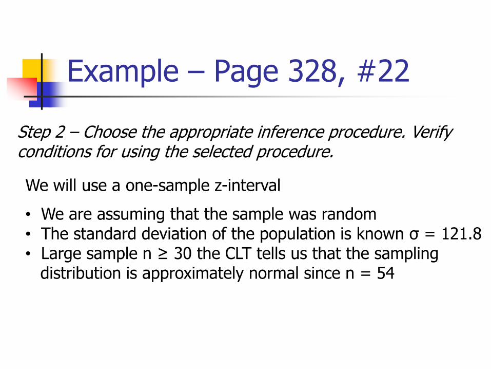
Step 2 – Choose the appropriate inference procedure. Verify conditions for using the selected procedure.
• We are assuming that the sample was random• The standard deviation of the population is known σ = 121.8• Large sample n ≥ 30 the CLT tells us that the sampling
distribution is approximately normal since n = 54
We will use a one-sample z-interval
Example – Page 328, #22
54
182.9
121.8
.99
n
x
CI
2α
σx z
n 121.8
182.9 2.57554
0.99
0.0050.005
0z 2.575 2.575
140.2 lbs < μ < 225.6 lbs
Step 3 – Carry out the inference procedure
Example – Page 328, #22
We are 99% confident that the mean weight of bears in Yellowstone National Park is between 140.2 lbsand 225.6 lbs.
Step 4 – Interpret you results in the context problem.

Lesson 6-4, Part 1
Estimating a Population mean: σ Not Known
Assumptions
Sample is a simple random sample
Values of the population standard deviation σ is unknown
The population is normally distributed or n > 30.
Student t Distribution
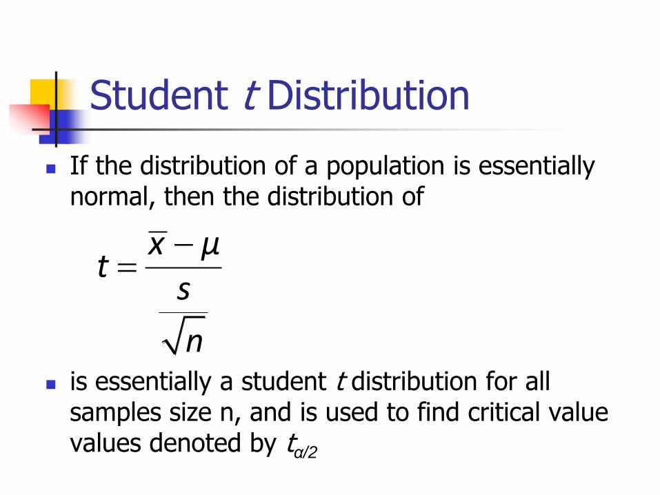
If the distribution of a population is essentially normal, then the distribution of
is essentially a student t distribution for all samples size n, and is used to find critical value values denoted by tα/2
x μt
s
n
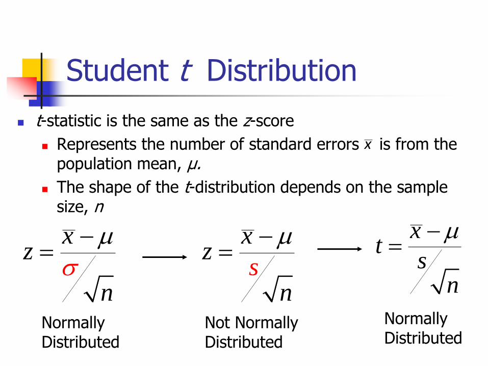
Student t Distribution
xz
n
xz
ns
xt
sn
Normally Distributed
Not Normally Distributed
Normally Distributed
t-statistic is the same as the z-score
Represents the number of standard errors is from the population mean, μ.
The shape of the t-distribution depends on the sample size, n
x
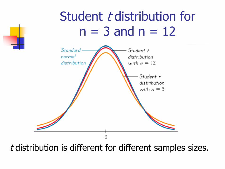
Student t distribution for n = 3 and n = 12
t distribution is different for different samples sizes.
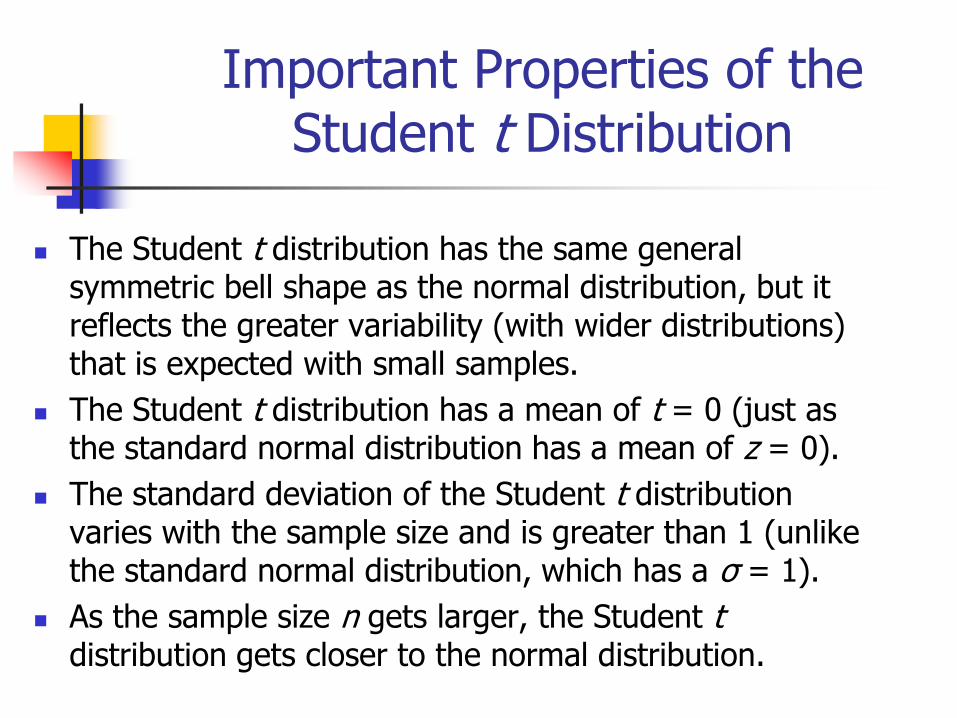
Important Properties of the Student t Distribution
The Student t distribution has the same general symmetric bell shape as the normal distribution, but it reflects the greater variability (with wider distributions) that is expected with small samples.
The Student t distribution has a mean of t = 0 (just as the standard normal distribution has a mean of z = 0).
The standard deviation of the Student t distribution varies with the sample size and is greater than 1 (unlike the standard normal distribution, which has a σ = 1).
As the sample size n gets larger, the Student t distribution gets closer to the normal distribution.
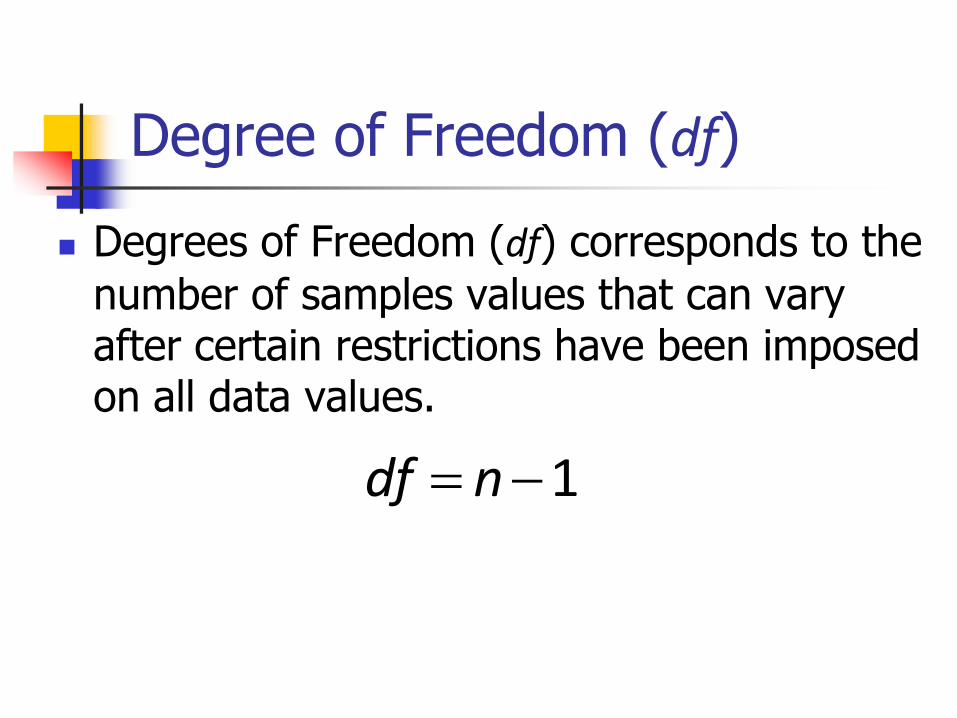
Degree of Freedom (df)
Degrees of Freedom (df) corresponds to the
number of samples values that can vary after certain restrictions have been imposed on all data values.
1df n
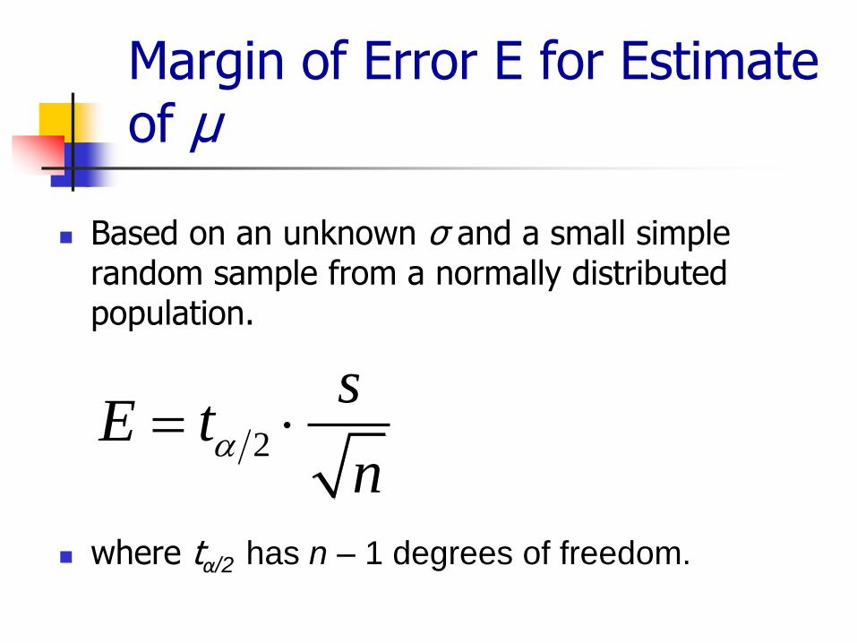
Margin of Error E for Estimate of μ
Based on an unknown σ and a small simple random sample from a normally distributed population.
where tα/2 has n – 1 degrees of freedom.
2
sE t
n
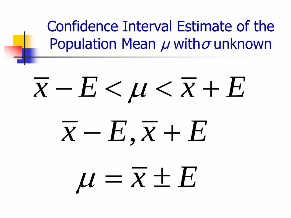
Confidence Interval Estimate of the Population Mean μ withσ unknown
x E x E
x E
, x E x E
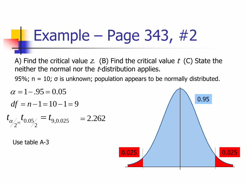
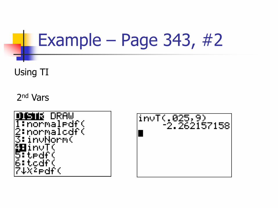
Example – Page 343, #2
A) Find the critical value z. (B) Find the critical value t (C) State theneither the normal nor the t-distribution applies.
95%; n = 10; σ is unknown; population appears to be normally distributed.
1 .95 0.05
1 10 1 9df n
0.05 9,0.0252 2
t t t
Use table A-3
2.262
0.025 0.025
0.95
Example – Page 343, #2
Using TI
2nd Vars
0.01 0.01
0.98
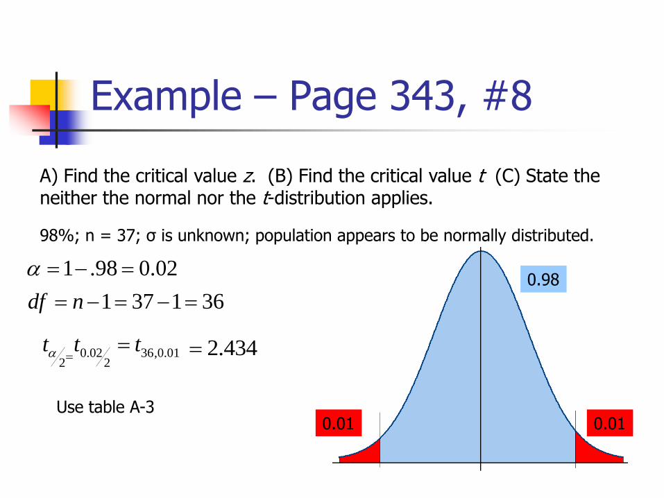
Example – Page 343, #8
A) Find the critical value z. (B) Find the critical value t (C) State theneither the normal nor the t-distribution applies.
98%; n = 37; σ is unknown; population appears to be normally distributed.
1 .98 0.02
1 37 1 36df n
0.02 36,0.012 2
t t t
Use table A-3
2.434
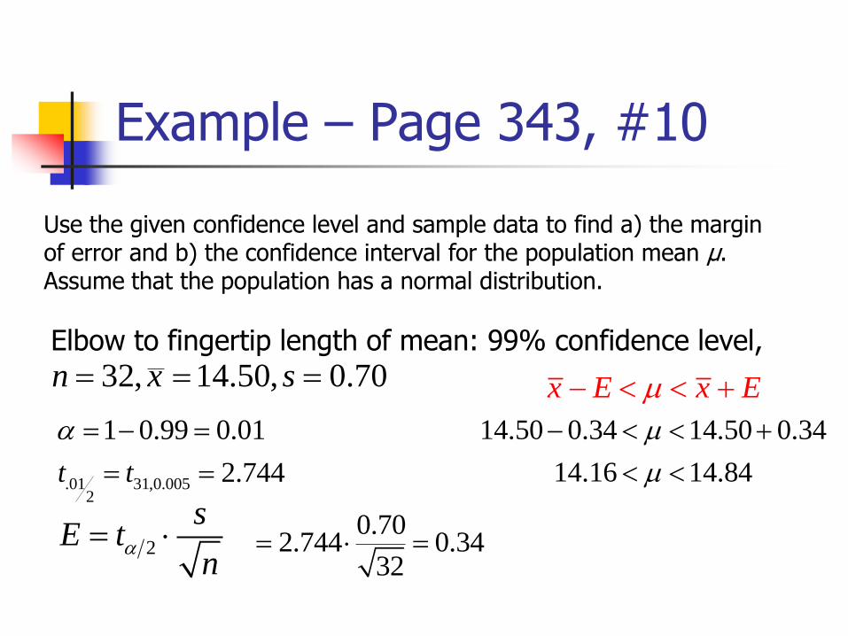
Example – Page 343, #10
2
sE t
n
Use the given confidence level and sample data to find a) the marginof error and b) the confidence interval for the population mean μ. Assume that the population has a normal distribution.
Elbow to fingertip length of mean: 99% confidence level,
32, 14.50, 0.70n x s
.01 31,0.0052
1 0.99 0.01
2.744t t
0.702.744 0.34
32
x E x E
14.50 0.34 14.50 0.34
14.16 14.84
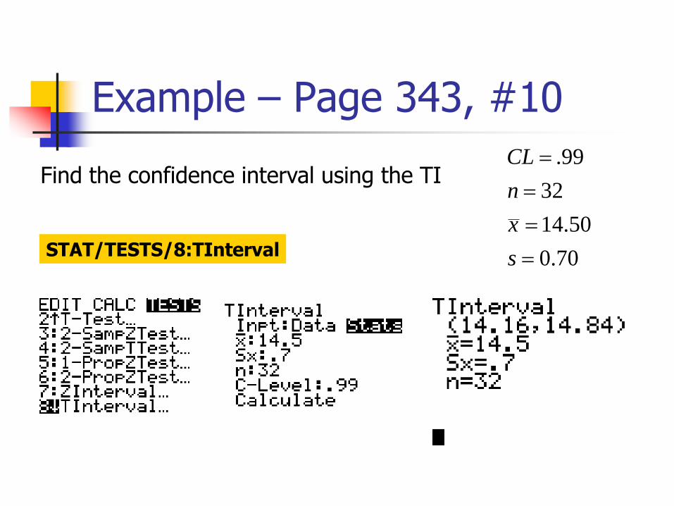
Example – Page 343, #10
.99
32
14.50
0.70
CL
n
x
s
Find the confidence interval using the TI
STAT/TESTS/8:TInterval
Lesson 6-4, Part 2
Estimating a Population mean: σ Not Known
Procedure for Constructing a Confidence Interval for μ, when σ is Unknown
Identify the population of interest and the parameter you want to draw conclusion about.
Choose the appropriate inference procedure. Verify the conditions for using the selected procedure.
Carry out the inference.
Interpret your results in the context of the problem.
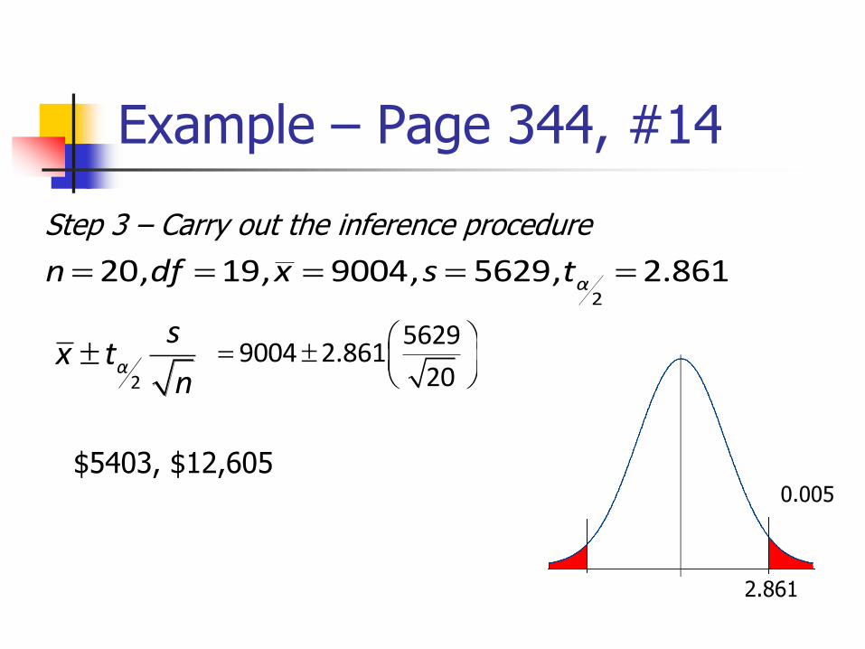
Example – Page 344, #14
A study was conducted to estimate hospital costs for accident victimswho wore seats belts. Twenty randomly selected cases have a distribution that appears to be bell-shape with a mean of $9004 anda standard deviation of $5629.
A) Construction the 99% confidence interval for the mean of all suchcosts.
µ = mean costs of accident victims who wore seat belts.
Step 1 – Identify the population of interest and the parameteryou want to draw conclusion about.
Example – Page 344, #14
Step 2 – Choose the appropriate inference procedure. Verifyconditions for using the selected procedure.
We will use a one-sample t-interval for the mean
• Random Sample – Stated in the question• Value of σ is unknown• Question stated that the distribution appears to be approximately normal
Example – Page 344, #14
220, 19, 9004, 5629, 2.861αn df x s t
0.005
2.861
2α
sx t
n
56299004 2.861
20
$5403, $12,605
Step 3 – Carry out the inference procedure
Example – Page 344, #14
We are 99% confident that the mean costs of all accidents victims who wear seat belts is between $5403 and $12605
Step 4 – Interpret your results in the context of the problem.
Example – Page 344, #14
B). If you are a manager for an insurance company that provides lowerrates for drivers who wear seat belts, and you want a conservative estimate for a worst scenario, what amount should youuse as the possible hospital cost for an accident victim who wearsseat belts?
$12,605 is the high end estimate for the long-runaverage hospital cost of such accident victims.
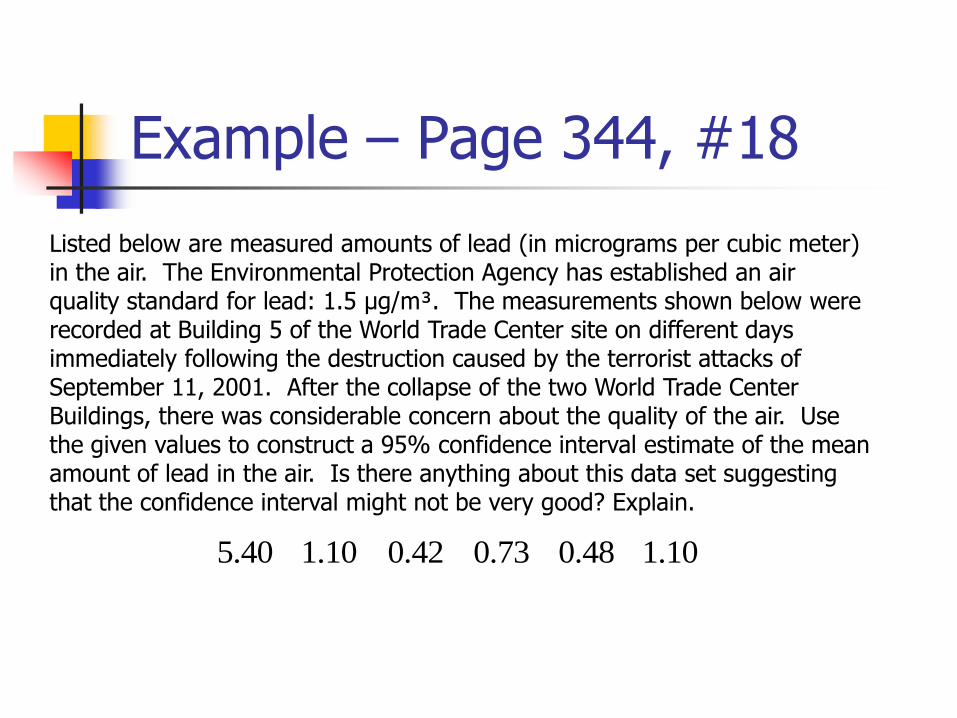
Example – Page 344, #18
Listed below are measured amounts of lead (in micrograms per cubic meter)in the air. The Environmental Protection Agency has established an airquality standard for lead: 1.5 μg/m³. The measurements shown below wererecorded at Building 5 of the World Trade Center site on different daysimmediately following the destruction caused by the terrorist attacks ofSeptember 11, 2001. After the collapse of the two World Trade Center Buildings, there was considerable concern about the quality of the air. Usethe given values to construct a 95% confidence interval estimate of the meanamount of lead in the air. Is there anything about this data set suggestingthat the confidence interval might not be very good? Explain.
5.40 1.10 0.42 0.73 0.48 1.10
Example – Page 344, #18
Step 1 – Identify the population of interest and the parameter you want to draw conclusions about.
µ = mean amount of lead in the air at the world Trade Center
Example – Page 344, #18
Choose the appropriate inference procedure. Verify conditions for using the selected procedure.
Use a one sample t-interval
• Measurements were not randomly selected, but its representative sample.
• The value of σ is unknown• The sampling distribution does not appear to be approximately normal since the box plot is skewed rightwith an outlier (see graph).

Example – Page 344, #18
Mean_Amt_of_Lead_at_the_World_Trade_Center
0 1 2 3 4 5 6
Collection 1 Box Plot
Example – Page 344, #18
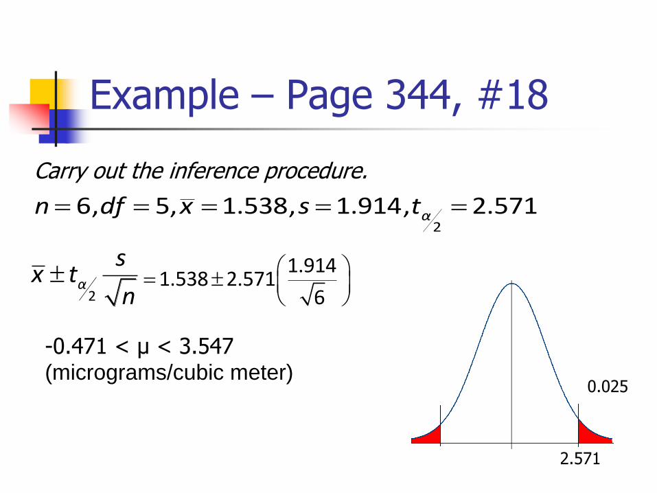
26, 5, 1.538, 1.914, 2.571αn df x s t
0.025
2.571
2α
sx t
n 1.914
1.538 2.5716
-0.471 < µ < 3.547 (micrograms/cubic meter)
Carry out the inference procedure.
Example – Page 344, #18
We are 95% confident that the mean lead amount of all air at the World Trade Center is between -0.4705 and 3.5472 (micrograms/cubic meter).
Yes, 4 of the 5 samples are below raises a question about whether the data meets the requirements that underlying population distribution is normal.
x
Step 4 – Interpret your results in the context of the problem.

Lesson 6-5
Estimating the Population Variance σ²
What is variance?
Is the difference between each observation and the mean.
Since the mean represents the “center of gravity,” the sum of all deviation about the mean must equal zero.
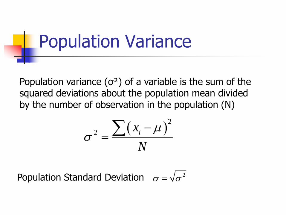
Population Variance
Population variance (σ²) of a variable is the sum of thesquared deviations about the population mean dividedby the number of observation in the population (N)
2
2 ix
N
Population Standard Deviation 2
Assumptions
The sample is simple random sample
The population must have normally distributed values (even if the sample is large).
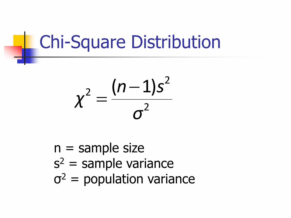
Chi-Square Distribution
22
2
( 1)n sχ
σ
n = sample sizes2 = sample varianceσ2 = population variance
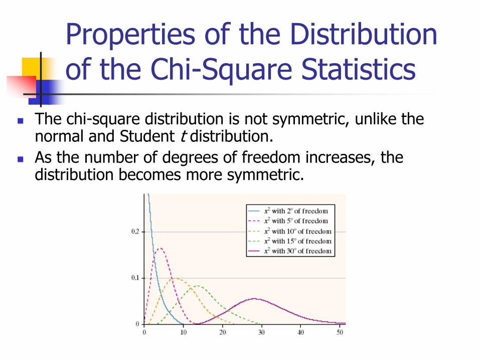
Properties of the Distribution of the Chi-Square Statistics
The chi-square distribution is not symmetric, unlike the normal and Student t distribution.
As the number of degrees of freedom increases, the distribution becomes more symmetric.
Properties of the Distribution of the Chi-Square Statistics
The values of chi-square can be zero or positive, but they cannot be negative.
The chi-square distribution is different for each number of degrees of freedom, which is df = n – 1 in this section. As the number increases, the chi-square distribution approaches a normal distribution.
In table A-4, each critical value of corresponds to an area given in the top row of the table, and that area represents the total region located to the right of the critical value.
2χ
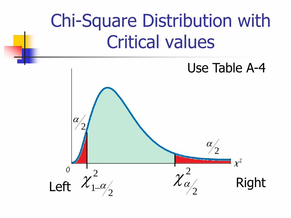
Chi-Square Distribution with Critical values
2
2
12
2
2
2
Use Table A-4
Left Right
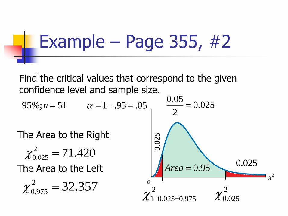
Example – Page 355, #2
Find the critical values that correspond to the given confidence level and sample size.
95%; 51n 1 .95 .05 0.05
0.0252
0.0250.95Area The Area to the Left
2
0.0252
0.975 32.357 2
1 0.025 0.975
2
0.025 71.420
The Area to the Right
0.0
25
Estimators of σ2
The sample variance s² is the best point estimate of the population variance σ²
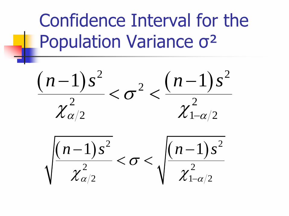
Confidence Interval for the Population Variance σ²
2 2
2
2 2
2 1 2
1 1n s n s
2 2
2 2
2 1 2
1 1n s n s
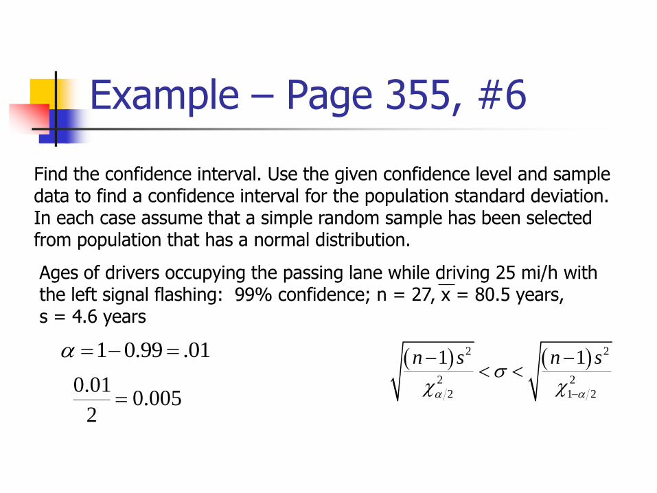
Example – Page 355, #6
Find the confidence interval. Use the given confidence level and sampledata to find a confidence interval for the population standard deviation.In each case assume that a simple random sample has been selectedfrom population that has a normal distribution.
Ages of drivers occupying the passing lane while driving 25 mi/h withthe left signal flashing: 99% confidence; n = 27, x = 80.5 years,s = 4.6 years
2 2
2 2
2 1 2
1 1n s n s
1 0.99 .01
0.010.005
2
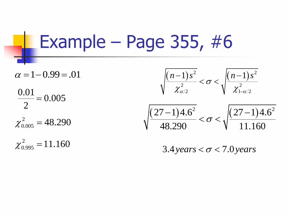
Example – Page 355, #6
2 2
2 2
2 1 2
1 1n s n s
1 0.99 .01
0.010.005
2
2
0.005 48.290
2
0.995 11.160
2 227 1 4.6 27 1 4.6
48.290 11.160
3.4 7.0years years
Procedure for Constructing a Confidence Interval for σ
Identify the population of interest and the parameter you want to draw conclusion about.
Choose the appropriate inference procedure. Verify the conditions for using the selected procedure.
Carry out the inference.
Interpret your results in the context of the problem.
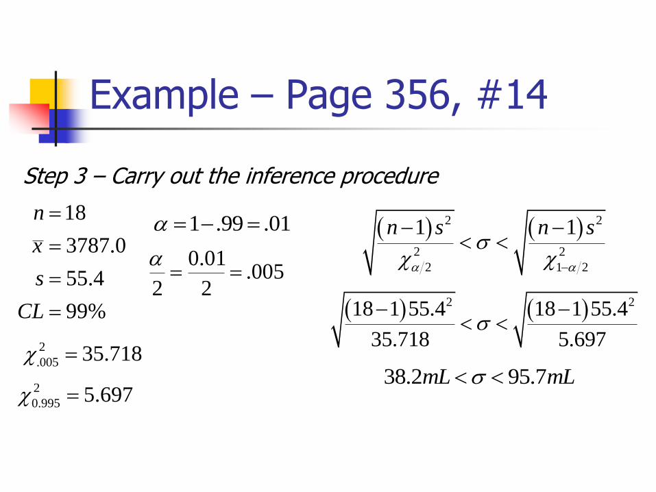
Example – Page 356, #14
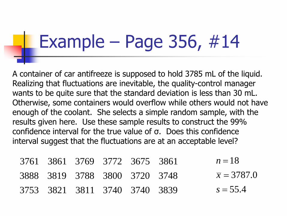
A container of car antifreeze is supposed to hold 3785 mL of the liquid.Realizing that fluctuations are inevitable, the quality-control managerwants to be quite sure that the standard deviation is less than 30 mL.Otherwise, some containers would overflow while others would not haveenough of the coolant. She selects a simple random sample, with theresults given here. Use these sample results to construct the 99%confidence interval for the true value of σ. Does this confidenceinterval suggest that the fluctuations are at an acceptable level?
3761 3861 3769 3772 3675 3861
3888 3819 3788 3800 3720 3748
3753 3821 3811 3740 3740 3839
18
3787.0
55.4
n
x
s
Example – Page 356, #14
σ = standard deviation of car antifreeze.
Use a chi-square interval
Conditions
Question stated SRS Since the histogram is approximately normal.
Step 1 – Identify the population of interest and the parameteryou want to draw conclusions about.
Step 2 – Choose the appropriate inference procedure. Verify conditions for using selected procedure.
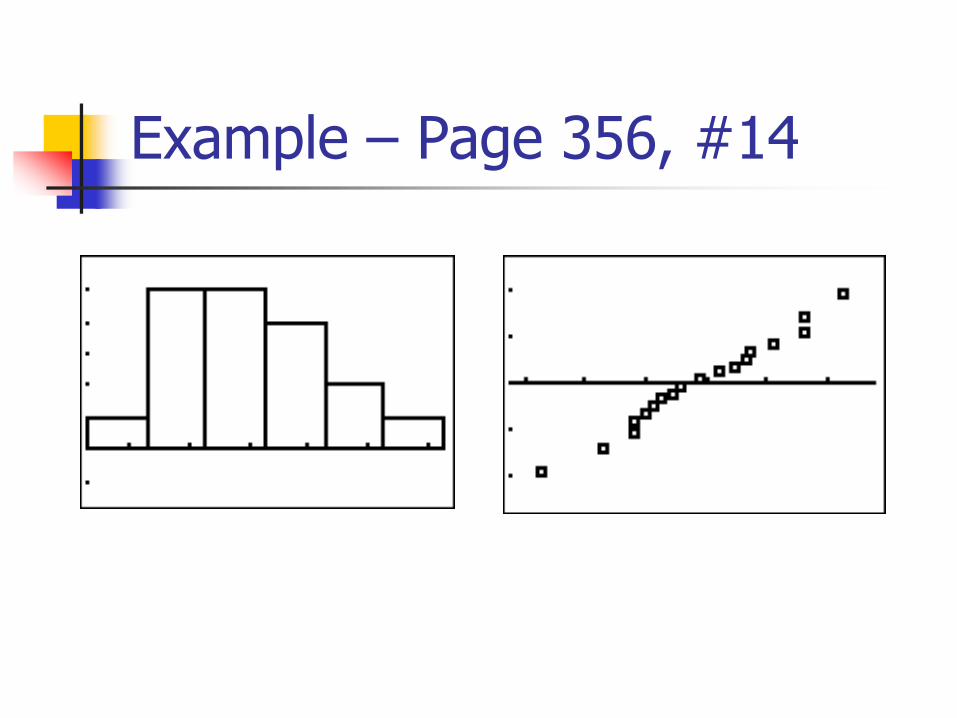
Example – Page 356, #14
Example – Page 356, #14
2 2
2 2
2 1 2
1 1n s n s
18
3787.0
55.4
99%
n
x
s
CL
1 .99 .01
0.01.005
2 2
2 218 1 55.4 18 1 55.4
35.718 5.697
2
.005 35.718
2
0.995 5.697 38.2 95.7mL mL
Step 3 – Carry out the inference procedure
Example – Page 356, #14
No, the interval indicates 99% confidence that σ > 30 mL (the fluctuations appears to be too high).
We are 99% confident that the standard deviation of car antifreeze is between 38.2 ml and 95.7 ml.
Step 4 – Interpret your results in the context of the problem.