Embed Size (px)
Citation preview

Continuous Random Variables 123
Copyright © 2013 Pearson Education, Inc.
Continuous Random Variables 5.2 The uniform distribution is sometimes referred to as the randomness distribution. 5.4 From Exercise 5.3, f(x) = 1/20 = .05 (10 ≤ x ≤ 30) a. P(10 ≤ x ≤ 25) = (25 − 10)(.05) = .75 b. P(20 < x < 30) = (30 − 20)(.05) = .5 c. P(x ≥ 25) = (30 − 25)(.05) = .25 d. P(x ≤ 10) = (10 − 10)(.05) = 0 e. P(x ≤ 25) = (25 − 10)(.05) = .75 f. P(20.5 ≤ x ≤ 25.5) = (25.5 − 20.5)(.05) = .25
5.6 From Exercise 5.5, 1
( )2
f x = (2 ≤ x ≤ 4)
a. 1
( ) .5 (4 ) .52
P x a a⎛ ⎞≥ = ⇒ − =⎜ ⎟⎝ ⎠
4 1
3
a
a
⇒ − =⇒ =
b. 1
( ) .2 ( 2) .22
P x a a⎛ ⎞≤ = ⇒ − =⎜ ⎟⎝ ⎠
2 .4
2.4
a
a
⇒ − =⇒ =
c. 1
( ) 0 ( 2) 02
P x a a⎛ ⎞≤ = ⇒ − =⎜ ⎟⎝ ⎠
2 0
2 or any number less than 2
a
a
⇒ − =⇒ =
d. 1
(2.5 ) .5 ( 2.5) .52
P x a a⎛ ⎞≤ ≤ = ⇒ − =⎜ ⎟⎝ ⎠
2.5 1
3.5
a
a
⇒ − =⇒ =
Chapter
5
124 Chapter 5
Copyright © 2013 Pearson Education, Inc.
5.8 50 100 1002
c dc d c dµ += = ⇒ + = ⇒ = −
5 5 1212
d cd cσ −= = ⇒ − =
Substituting, (100 ) 5 12 2 100 5 12d d d− − = ⇒ − =
2 100 5 12
100 5 12
258.66
d
d
d
⇒ = +
+⇒ =
⇒ =
Since 100 58.66 100c d c+ = ⇒ + = 41.34c⇒ =
f(x) = ( )1( )f x c x d
d c= ≤ ≤
−
1 1 1
.05858.66 41.34 17.32d c
= = =− −
Therefore, .058 41.34 58.66
( )0 otherwise
xf x
≤ ≤⎧= ⎨⎩
The graph of the probability distribution for x is given here.
x
f(x)
605040
0.20
0.15
0.10
0.05
0.00
5.10 We are given that x is a uniform random variable on the interval from 0 to 3,600 seconds.
Therefore, c = 0 and d = 3,600. The last 15 minutes would represent 15(60) = 900 seconds and would represents seconds 2700 to 3600.
3600 2700 900
( 2700) .253600 0 3600
P x−> = = =
−
Continuous Random Variables 125
Copyright © 2013 Pearson Education, Inc.
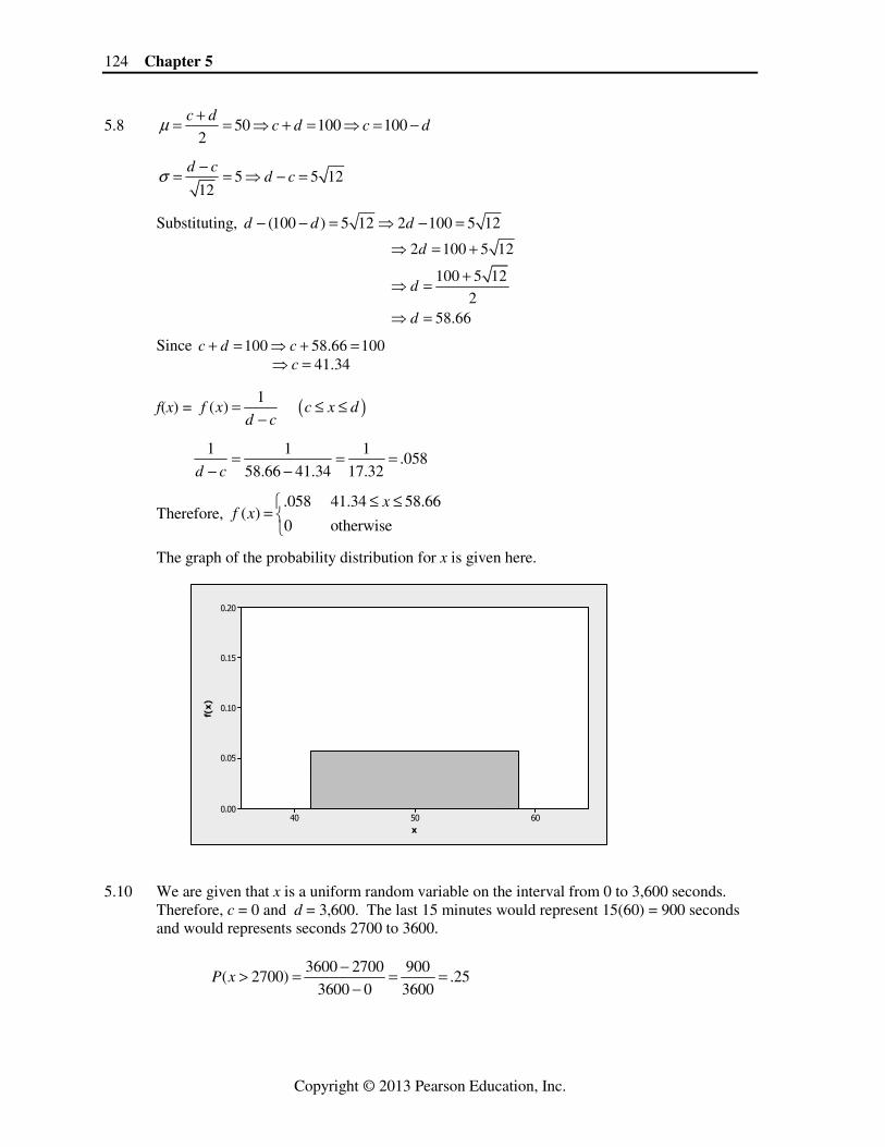
5.12 Using MINITAB, the histogram of the data is:
RANUNI
Freq
uenc
y
100806040200
5
4
3
2
1
0
The histogram looks like the data could come from a uniform distribution. There is
some variation in the height of the bars, but we cannot expect a perfect graph from a sample of only 40 observations.
5.14 a. Since x is a uniform random variable on the interval from 0 to 1, c = 0 and d = 1.
0 1 1
( ) .52 2 2
c dE x
+ += = = =
b. 1 .7 .3
( .7) .31 0 1
P x−> = = =−
c. If there are only 2 members, then there is only 1 possible connection. The density will
then be either 0 or 1. The density would be a discrete random variable, not continuous. Therefore, the uniform distribution would not be appropriate.
5.16 Let x = length of time a bus is late. Then x is a uniform random variable with probability
distribution:
1
(0 20)( ) 20
0 otherwise
xf x
⎧ ≤ ≤⎪= ⎨⎪⎩
a. 0 20
102
µ += =
b. 1 1
( 19) (20 19) .0520 20
P x⎛ ⎞≥ = − = =⎜ ⎟⎝ ⎠
c. It would be doubtful that the director’s claim is true, since the probability of the being
more than 19 minutes late is so small.

126 Chapter 5
Copyright © 2013 Pearson Education, Inc.
5.18 a.
p
f(p)
10
1
0
b. 0 1
.52 2
c dµ + += = =
1 0
.28912 12
d cσ − −= = = 2 2.289 .083σ = =
c. ( .95) (1 .95)(1) .05P p > = − = ( .95) (.95 0)(1) .95P p < = − = d. The analyst should use a uniform probability distribution with c = .90 and d = .95.
1 1 1
20 (.90 .95)( ) .95 .90 .05
0 otherwise
pf p d c
⎧ = = = ≤ ≤⎪= − −⎨⎪⎩
5.20 A normal distribution is a bell-shaped curve with the center of the distribution at µ . 5.22 If x has a normal distribution with mean µ and standard deviationσ , then the distribution of
σµ−= x
z is a normal with a mean of 0µ = and a standard deviation of 1σ = .
5.24 a. ( 2.00 0) .4772P z− < < = (from Table IV, Appendix A) b. ( 1.00 0) .3413P z− < < = (from Table IV, Appendix A)

Continuous Random Variables 127
Copyright © 2013 Pearson Education, Inc.
c. ( 1.69 0) .4545P z− < < = (from Table IV, Appendix A) d. ( .58 0) .2190P z− < < = (from Table IV, Appendix A) 5.26 Using Table IV, Appendix A: a. ( 1.46) .5 (0 1.46)P z P z> = − < ≤ .5 .4279 .0721= − = b. ( 1.56) .5 ( 1.56 0)P z P z< − = − − ≤ < .5 .4406 .0594= − = c. (.67 2.41)P z≤ ≤
(0 2.41) (0 .67)
.4920 .2486 .2434
P z P z= < ≤ − < <= − =
d. ( 1.96 .33)P z− ≤ < −
( 1.96 0) ( .33 0)
.4750 .1293 .3457
P z P z= − ≤ < − − ≤ <= − =
e. ( 0) .5P z ≥ = f. ( 2.33 1.50)P z− < <
( 2.33 0) (0 1.50)
.4901 .4332 .9233
P z P z= − < < + < <= + =
128 Chapter 5
Copyright © 2013 Pearson Education, Inc.
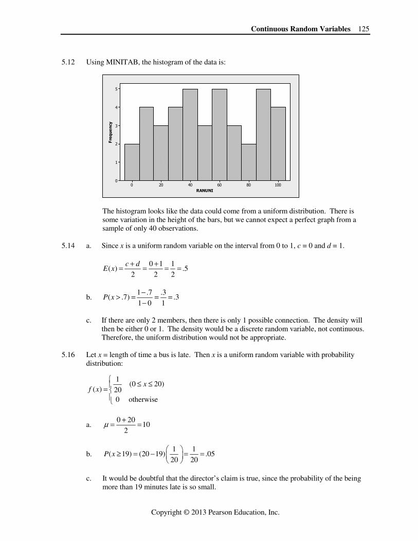
g. ( 2.33) ( 2.33 0) ( 0)P z P z P z≥ − = − ≤ ≤ + ≥
.4901 .5000
.9901
= +=
h. ( 2.33) ( 0) (0 2.33)P z P z P z< = ≤ + ≤ ≤
.5000 .4901
.9901
= +=
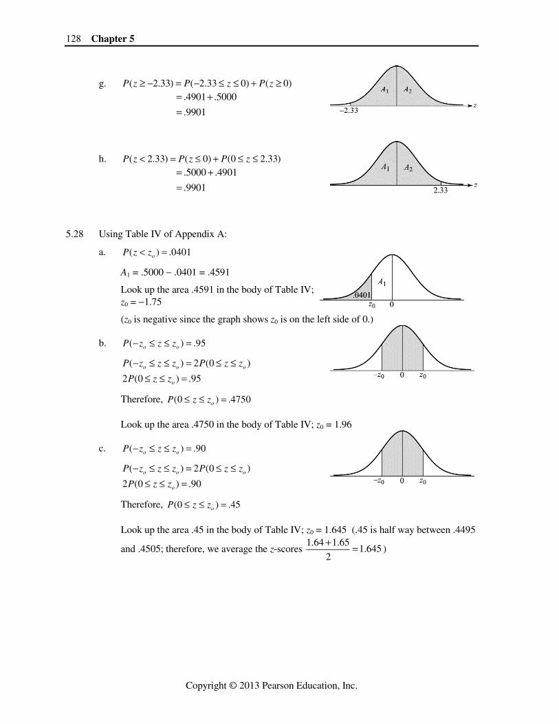
5.28 Using Table IV of Appendix A: a. ( ) .0401oP z z< = A1 = .5000 − .0401 = .4591 Look up the area .4591 in the body of Table IV; z0 = −1.75 (z0 is negative since the graph shows z0 is on the left side of 0.) b. ( ) .95o oP z z z− ≤ ≤ =
( ) 2 (0 )
2 (0 ) .95o o o
o
P z z z P z z
P z z
− ≤ ≤ = ≤ ≤≤ ≤ =
Therefore, (0 ) .4750oP z z≤ ≤ = Look up the area .4750 in the body of Table IV; z0 = 1.96 c. ( ) .90o oP z z z− ≤ ≤ =
( ) 2 (0 )
2 (0 ) .90o o o
o
P z z z P z z
P z z
− ≤ ≤ = ≤ ≤≤ ≤ =
Therefore, (0 ) .45oP z z≤ ≤ = Look up the area .45 in the body of Table IV; z0 = 1.645 (.45 is half way between .4495
and .4505; therefore, we average the z-scores 1.64 1.65
1.6452
+ = )
Continuous Random Variables 129
Copyright © 2013 Pearson Education, Inc.
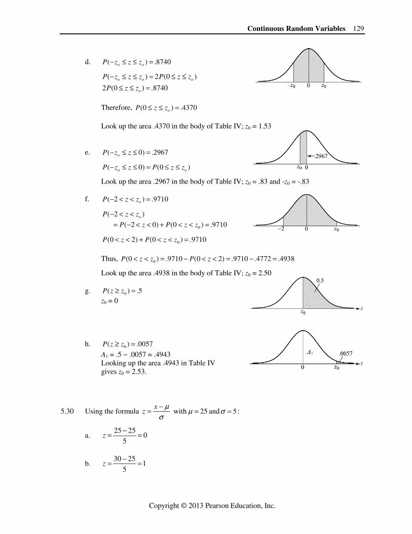
d. ( ) .8740o oP z z z− ≤ ≤ =
( ) 2 (0 )
2 (0 ) .8740o o o
o
P z z z P z z
P z z
− ≤ ≤ = ≤ ≤≤ ≤ =
Therefore, (0 ) .4370oP z z≤ ≤ =
Look up the area .4370 in the body of Table IV; z0 = 1.53
e. ( 0) .2967oP z z− ≤ ≤ = ( 0) (0 )o oP z z P z z− ≤ ≤ = ≤ ≤ Look up the area .2967 in the body of Table IV; z0 = .83 and -z0 = -.83 f. ( 2 ) .9710oP z z− < < = ( 2 )oP z z− < <
0( 2 0) (0 ) .9710P z P z z= − < < + < < = 0(0 2) (0 ) .9710P z P z z< < + < < = Thus, 0(0 ) .9710 (0 2) .9710 .4772 .4938P z z P z< < = − < < = − = Look up the area .4938 in the body of Table IV; z0 = 2.50 g. 0( ) .5P z z≥ = z0 = 0 h. 0( ) .0057P z z≥ =
A1 = .5 − .0057 = .4943 Looking up the area .4943 in Table IV gives z0 = 2.53.
5.30 Using the formula x
zµ
σ−= with 25µ = and 5σ = :
a. 25 25
05
z−= =
b. 30 25
15
z−= =
130 Chapter 5
Copyright © 2013 Pearson Education, Inc.
c. 37.5 25
2.55
z−= =
d. 10 25
35
z−= = −
e. 50 25
55
z−= =
f. 32 25
1.45
z−= =
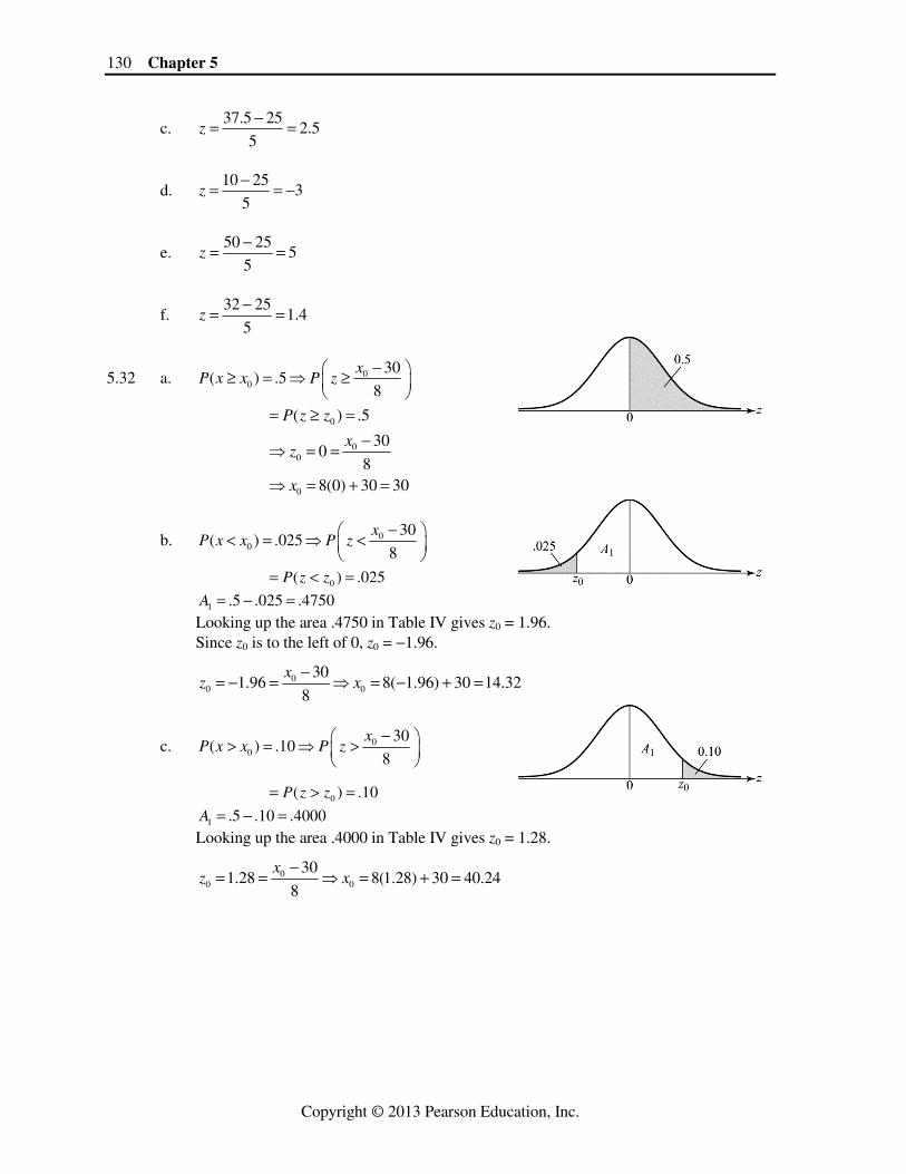
5.32 a. 00
30( ) .5
8
xP x x P z
−⎛ ⎞≥ = ⇒ ≥⎜ ⎟⎝ ⎠
0
00
0
( ) .5
300
88(0) 30 30
P z z
xz
x
= ≥ =−
⇒ = =
⇒ = + =
b. 00
30( ) .025
8
xP x x P z
−⎛ ⎞< = ⇒ <⎜ ⎟⎝ ⎠
0( ) .025P z z= < =
1 .5 .025 .4750A = − = Looking up the area .4750 in Table IV gives z0 = 1.96. Since z0 is to the left of 0, z0 = −1.96.
00 0
301.96 8( 1.96) 30 14.32
8
xz x
−= − = ⇒ = − + =
c. 00
30( ) .10
8
xP x x P z
−⎛ ⎞> = ⇒ >⎜ ⎟⎝ ⎠
0( ) .10P z z= > =
1 .5 .10 .4000A = − = Looking up the area .4000 in Table IV gives z0 = 1.28.
00 0
301.28 8(1.28) 30 40.24
8
xz x
−= = ⇒ = + =
Continuous Random Variables 131
Copyright © 2013 Pearson Education, Inc.
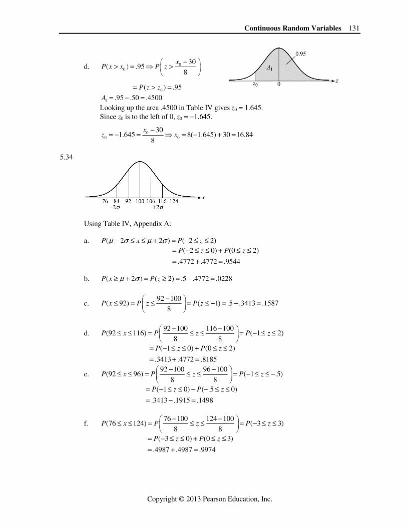
d. 00
30( ) .95
8
xP x x P z
−⎛ ⎞> = ⇒ >⎜ ⎟⎝ ⎠
0( ) .95P z z= > =
1 .95 .50 .4500A = − = Looking up the area .4500 in Table IV gives z0 = 1.645. Since z0 is to the left of 0, z0 = −1.645.
00 0
301.645 8( 1.645) 30 16.84
8
xz x
−= − = ⇒ = − + =
5.34
Using Table IV, Appendix A: a. ( 2 2 ) ( 2 2)P x P zµ σ µ σ− ≤ ≤ + = − ≤ ≤
( 2 0) (0 2)
.4772 .4772 .9544
P z P z= − ≤ ≤ + ≤ ≤= + =
b. ( 2 ) ( 2) .5 .4772 .0228P x P zµ σ≥ + = ≥ = − =
c. 92 100
( 92) ( 1) .5 .3413 .15878
P x P z P z−⎛ ⎞≤ = ≤ = ≤ − = − =⎜ ⎟
⎝ ⎠
d. 92 100 116 100
(92 116) ( 1 2)8 8
P x P z P z− −⎛ ⎞≤ ≤ = ≤ ≤ = − ≤ ≤⎜ ⎟
⎝ ⎠
( 1 0) (0 2)
.3413 .4772 .8185
P z P z= − ≤ ≤ + ≤ ≤= + =
e. 92 100 96 100
(92 96) ( 1 .5)8 8
P x P z P z− −⎛ ⎞≤ ≤ = ≤ ≤ = − ≤ ≤ −⎜ ⎟
⎝ ⎠
( 1 0) ( .5 0)
.3413 .1915 .1498
P z P z= − ≤ ≤ − − ≤ ≤= − =
f. 76 100 124 100
(76 124) ( 3 3)8 8
P x P z P z− −⎛ ⎞≤ ≤ = ≤ ≤ = − ≤ ≤⎜ ⎟
⎝ ⎠
( 3 0) (0 3)
.4987 .4987 .9974
P z P z= − ≤ ≤ + ≤ ≤= + =

132 Chapter 5
Copyright © 2013 Pearson Education, Inc.
5.36 a. ( 2 ) ( 2 ) ( 2) ( 2)P x P x P z P zµ σ µ σ< − + > + = < − + >
(.5 .4772) (.5 .4772)
2(.5 .4772) .0456
= − + −= − =
(from Table IV, Appendix A)
( 3 ) ( 3 ) ( 3) ( 3)P x P x P z P zµ σ µ σ< − + > + = < − + >
(.5 .4987) (.5 .4987)
2(.5 .4987) .0026
= − + −= − =
(from Table IV, Appendix A)
b. ( ) ( 1 1)P x P zµ σ µ σ− < < + = − < <
( 1 0) (0 1)
.3413 .3413 2(.3413) .6826
P z P z= − < < + < <= + = =
(from Table IV, Appendix A)
( 2 2 ) ( 2 2)P x P zµ σ µ σ− < < + = − < <
( 2 0) (0 2)
.4772 .4772 2(.4772) .9544
P z P z= − < < + < <= + = =
(from Table IV, Appendix A)
c. 0( ) .80P x x≤ = . Find x0.
00 0
300( ) ( ) .80
30
xP x x P z P z z
−⎛ ⎞≤ = ≤ = ≤ =⎜ ⎟⎝ ⎠
1 .80 .50 .3000A = − = Looking up area .3000 in Table IV, z0 = .84.
0 00 0
300 300.84 325.2
30 30
x xz x
− −= ⇒ = ⇒ =
0( ) .10P x x≤ = . Find x0.
00 0
300( ) ( ) .10
30
xP x x P z P z z
−⎛ ⎞≤ = ≤ = ≤ =⎜ ⎟⎝ ⎠
1 .50 .10 .4000A = − = Looking up area .4000 in Table IV, z0 = −1.28.
0 00 0
300 3001.28 261.6
30 30
x xz x
− −= ⇒ − = ⇒ =
5.38 a. 120 105.3
( 120) ( 1.84)8
P x P z P z−⎛ ⎞> = > = >⎜ ⎟
⎝ ⎠
.5 (0 1.84) .5 .4671 .0329P z= − < < = − = (Using Table IV, Appendix A)
Continuous Random Variables 133
Copyright © 2013 Pearson Education, Inc.
b. 100 105.3 110 105.3
(100 110) ( .66 .59)8 8
P x P z P z− −⎛ ⎞< < = < < = − < <⎜ ⎟
⎝ ⎠
( .66 0) (0 .59) .2454 .2224 .4678P z P z= − < < + < < = + = (Using Table IV, Appendix A)
c. 105.3
( ) .25 ( ) .258 o
aP x a P z P z z
−⎛ ⎞< = ⇒ < = < =⎜ ⎟⎝ ⎠
1 .5 .25 .25A = − = Looking up the area .25 in Table IV gives zo = -.67.
105.3
.67 8( .67) 105.3 99.948o
az a
−= − = ⇒ = − + =
5.40 a. Using Table IV, Appendix A,
0 5.26
( 0) ( .53) .5000 .2019 .701910
P x P z P z−⎛ ⎞> = > = > − = + =⎜ ⎟
⎝ ⎠
b. 5 5.26 15 5.26
(5 15) ( .03 .97) .0120 .3340 .346010 10
P x P z P z− −⎛ ⎞< < = < < = − < < = + =⎜ ⎟
⎝ ⎠
c. 1 5.26
( 1) ( .43) .5000 .1664 .333610
P x P z P z−⎛ ⎞< = < = < − = − =⎜ ⎟
⎝ ⎠
d. 25 5.26
( 25) ( 3.03) .5000 .4988 .001210
P x P z P z− −⎛ ⎞< − = < = < − = − =⎜ ⎟
⎝ ⎠
Since the probability of seeing an average casino win percentage of -25% or smaller after 100 bets on black/red is so small (.0012), we would conclude that either the mean casino win percentage is not 5.26% but something smaller or the standard deviation of 10% is too small.
5.42 a. Let x = carapace length of green sea turtle. Then x has a normal distribution with
55.7µ = and 11.5σ = .
40 55.7 60 55.7( 40) ( 60)
11.5 11.5
( 1.37) ( .37)
.5 .4147 .5 .1443 .4410
P x P x P z P z
P z P z
− −⎛ ⎞ ⎛ ⎞< + > = < + >⎜ ⎟ ⎜ ⎟⎝ ⎠ ⎝ ⎠
= < − + >= − + − =
b. 55.7
( ) .10 ( ) .1011.5 o
LP x L P z P z z
−⎛ ⎞> = ⇒ > = > =⎜ ⎟⎝ ⎠
1 .5 .10 .40A = − =

134 Chapter 5
Copyright © 2013 Pearson Education, Inc.
Looking up the area .40 in Table IV gives zo = 1.28.
55.7
1.28 1.28(11.5) 55.7 70.4211.5o
Lz L
−= = ⇒ = + =
5.44 a. If the player aims at the right goal post, he will score if the ball is less than 3 feet away
from the goal post inside the goal (because the goalie is standing 12 feet from the goal post and can reach 9 feet). Using Table IV, Appendix A,
3 0
(0 3) 0 (0 1) .34133
P x P z P z−⎛ ⎞< < = < < = < < =⎜ ⎟
⎝ ⎠
b. If the player aims at the center of the goal, he will be aimed at the goalie. In order to
score, the player must place the ball more than 9 feet away from the goalie. Using Table IV, Appendix A
9 0 9 0
( 9) ( 9)3 3
( 3) ( 3) .5 .5 .5 .5 0
P x P x P z P z
P z P z
− − −⎛ ⎞ ⎛ ⎞< − + > = < + >⎜ ⎟ ⎜ ⎟⎝ ⎠ ⎝ ⎠
= < − + > ≈ − + − =
c. If the player aims halfway between the goal post and the goalie’s reach, he will be
aiming 1.5 feet from the goal post. Therefore, he will score if he hits from 1.5 feet to the left of where he is aiming to 1.5 feet to the right of where he is aiming. Using Table IV, Appendix A,
1.5 0 1.5 0
( 1.5 1.5)3 3
( .5 .5) .1915 .1915 .3830
P x P z
P z
− − −⎛ ⎞− < < = < <⎜ ⎟⎝ ⎠
= − < < = + =
5.46 a. Let x = rating of employee’s performance. Then x has a normal distribution with
50µ = and 15σ = . The top 10% get “exemplary” ratings.
50
( ) .10 ( ) .1015
oo o
xP x x P z P z z
−⎛ ⎞> = ⇒ > = > =⎜ ⎟⎝ ⎠
1 .5 .10 .40A = − = Looking up the area .40 in Table IV gives zo = 1.28.
50
1.28 1.28(15) 50 69.215
oo o
xz x
−= = ⇒ = + =
b. Only 30% of the employees will get ratings lower than “competent”.
50
( ) .30 ( ) .3015
oo o
xP x x P z P z z
−⎛ ⎞< = ⇒ < = < =⎜ ⎟⎝ ⎠
1 .5 .30 .20A = − =
Continuous Random Variables 135
Copyright © 2013 Pearson Education, Inc.
Looking up the area .20 in Table IV gives zo = -.52. The value of zo is negative because it is in the lower tail.
50
.52 .52(15) 50 42.215
oo o
xz x
−= − = ⇒ = − + =
5.48 a. Using Table IV, Appendix A,
40 37.9 50 37.9(40 50) (.17 .98)
12.4 12.4
.3365 .0675 .2690.
P x P z P z− −⎛ ⎞< < = < < = < <⎜ ⎟
⎝ ⎠= − =
b. Using Table IV, Appendix A,
30 37.9
( 30) ( .64) .5 .2389 .261112.4
P x P z P z−⎛ ⎞< = < = < − = − =⎜ ⎟
⎝ ⎠.
c. We know that if ( ) .95L UP z z z< < = , then ( 0) (0 ) .95L UP z z P z z< < + < < = and
( 0) (0 ) .95 / 2 .4750L UP z z P z z< < = < < = = . Using Table IV, Appendix A, zU = 1.96 and zL = -1.96.
UL 37.937.9( ) .95 .95
12.4 12.4L U
xxP x x x P z
−−⎛ ⎞< < = ⇒ < < =⎜ ⎟⎝ ⎠
L 37.91.96
12.4
x −⇒ = − and U 37.9
1.9612.4
x − =
37.9 24.3 and 37.9 24.3 13.6 and 62.2L U L Ux x x x⇒ − = − − = ⇒ = =
d. 0 0( ) .10 (0 ) .4000P z z P z z> = ⇒ < < = . Using Table IV, Appendix A, z0 = 1.28.
00 0 0
37.9( ) .10 1.28 37.9 15.9 53.8
12.4
xP x x x x
−> = ⇒ = ⇒ − = ⇒ = .
5.50 a. Let x = fill of container. Using Table IV, Appendix A,
10 10
( 10) ( 0) .5.2
P x P z P z−⎛ ⎞< = < = < =⎜ ⎟
⎝ ⎠
b. Profit = Price – cost – reprocessing fee = $230 − $20(10.6) − $10 = $230 − $212 − $10 = $8.
136 Chapter 5
Copyright © 2013 Pearson Education, Inc.
c. If the probability of underfill is approximately 0, then Profit = Price – Cost.
E(Profit) = E(Price − Cost) = $230 – E(Cost) = $230 − $20E(x) = $230 − $20(10.5) = $230 − $210 = $20.
5.52 Let x = load. From the problem, we know that the distribution of x is normal with a mean of
20.
0 0
10 20 30 20(10 30) ( ) .95P x P z P z z z
σ σ− −⎛ ⎞< < = < < = − < < =⎜ ⎟
⎝ ⎠
First, we need to find z0 such that 0 0( ) .95P z z z− < < = . Since we know that the center of the z distribution is 0, half of the area or .95/2 = .475 will be between –z0 and 0 and half will be between 0 and z0.
We look up .475 in the body of Table IV, Appendix A to find z0 = 1.96. Thus,
30 201.96
101.96 10 5.102
1.96
σ
σ σ
− =
⇒ = ⇒ = =
5.54 Four methods for determining whether the sample data come from a normal population are:
1. Use either a histogram or a stem-and-leaf display for the data and note the shape of the graph. If the data are approximately normal, then the graph will be similar to the normal curve.
2. Compute the intervals ,3 ,2 , sxsxsx ±±± and determine the percentage of measurements falling in each. If the data are approximately normal, the percentages will be approximately equal to 68%, 95%, and 100%, respectively.
3. Find the interquartile range, IQR, and the standard deviation, s, for the sample, then calculate the ratio IQR / s. If the data are approximately normal, then IQR / s ≈ 1.3.
4. Construct a normal probability plot for the data. If the data are approximately normal, the points will fall (approximately) on a straight line.
5.56 In a normal probability plot, the observations in a data set are ordered from smallest to largest
and then plotted against the expected z-scores of observations calculated under the assumption that the data come from a normal distribution. If the data are normally distributed, a linear or straight-line trend will result.
5.58 a. IQR = QU − QL = 195 − 72 = 123
b. IQR/s = 123/95 = 1.295 c. Yes. Since IQR is approximately 1.3, this implies that the data are approximately normal.
Continuous Random Variables 137
Copyright © 2013 Pearson Education, Inc.
5.60 a. Using MINITAB, the stem-and-leaf display of the data is:
Stem-and-Leaf Display: Data Stem-and-leaf of Data N = 28 Leaf Unit = 0.10 2 1 16 3 2 1 7 3 1235 11 4 0356 (4) 5 0399 13 6 03457 8 7 34 6 8 2446 2 9 47
The data are somewhat mound-shaped, so the data could be normally distributed.
b. Using MINITAB, the descriptive statistics are:
Descriptive Statistics: Data Variable N Mean StDev Minimum Q1 Median Q3 Maximum Data 28 5.596 2.353 1.100 3.625 5.900 7.375 9.700
From the printout, the standard deviation is s = 2.353.
c. From the printout, QL = 3.625 and QU = 7.375. The interquartile range is IQR = QU – QL = 7.375 – 3.625 = 3.75. If the data are approximately normal, then IQR / s ≈ 1.3. For this data, IQR / s = 3.75 / 2.353 = 1.397. This is fairly close to 1.3, so the data could be normal.
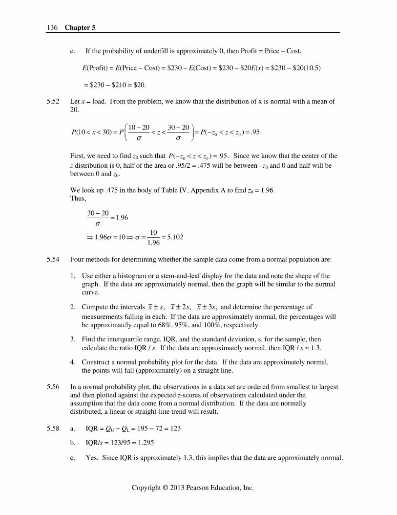
d. Using MINITAB, the normal probability plot is:
Data
Perc
ent
12.510.07.55.02.50.0
99
95
90
80
70
60504030
20
10
5
1
Mean
0.902
5.596StDev 2.353N 28AD 0.183P-Value
Probability P lot of DataNormal - 95% CI
Since the data are very close to a straight line, it indicates that the data could be
normally distributed.
138 Chapter 5
Copyright © 2013 Pearson Education, Inc.
5.62 The histogram of the data is mound-shaped. It is somewhat skewed to the right, so it is not exactly symmetric. However, it is very close to a mound shaped distribution, so the engineers could use the normal probability distribution to model the behavior of shear strength for rock fractures.
5.64 a. We know that approximately 68% of the observations will fall within 1 standard
deviation of the mean, approximately 95% will fall within 2 standard deviations of the mean, and approximately 100% of the observations will fall within 3 standard deviation of the mean. From the printout, the mean is 89.29 and the standard deviation is 3.18.
89.29 3.18 (86.11, 92.47)x s± ⇒ ± ⇒ . Of the 50 observations, 34 (or 34/50 = .68) fall
between 86.11 and 92.47. This is close to what we would expect if the data were normally distributed.
2 89.29 2(3.18) 89.29 6.36 (82.93, 95.65)x s± ⇒ ± ⇒ ± ⇒ . Of the 50 observations, 48
(or 48/50 = .96) fall between 82.93 and 95.65. This is close to what we would expect if the data were normally distributed.
3 89.29 3(3.18) 89.29 9.54 (79.75, 98.83)x s± ⇒ ± ⇒ ± ⇒ . Of the 50 observations, 50
(or 50/50 = 1.00) fall between 79.75 and 98.83. This is close to what we would expect if the data were normally distributed.
The IQR = 4.84 and s = 3.18344. The ratio of the IQR and s is 4.84
1.523.18344
IQR
s= = .
This is close to 1.3 that we would expect if the data were normally distributed. Thus, there is evidence that the data are normally distributed. b. If the data are normally distributed, the points will form a straight line when plotted
using a normal probability plot. From the normal probability plot, the data points are close to a straight line. There is evidence that the data are normally distributed.
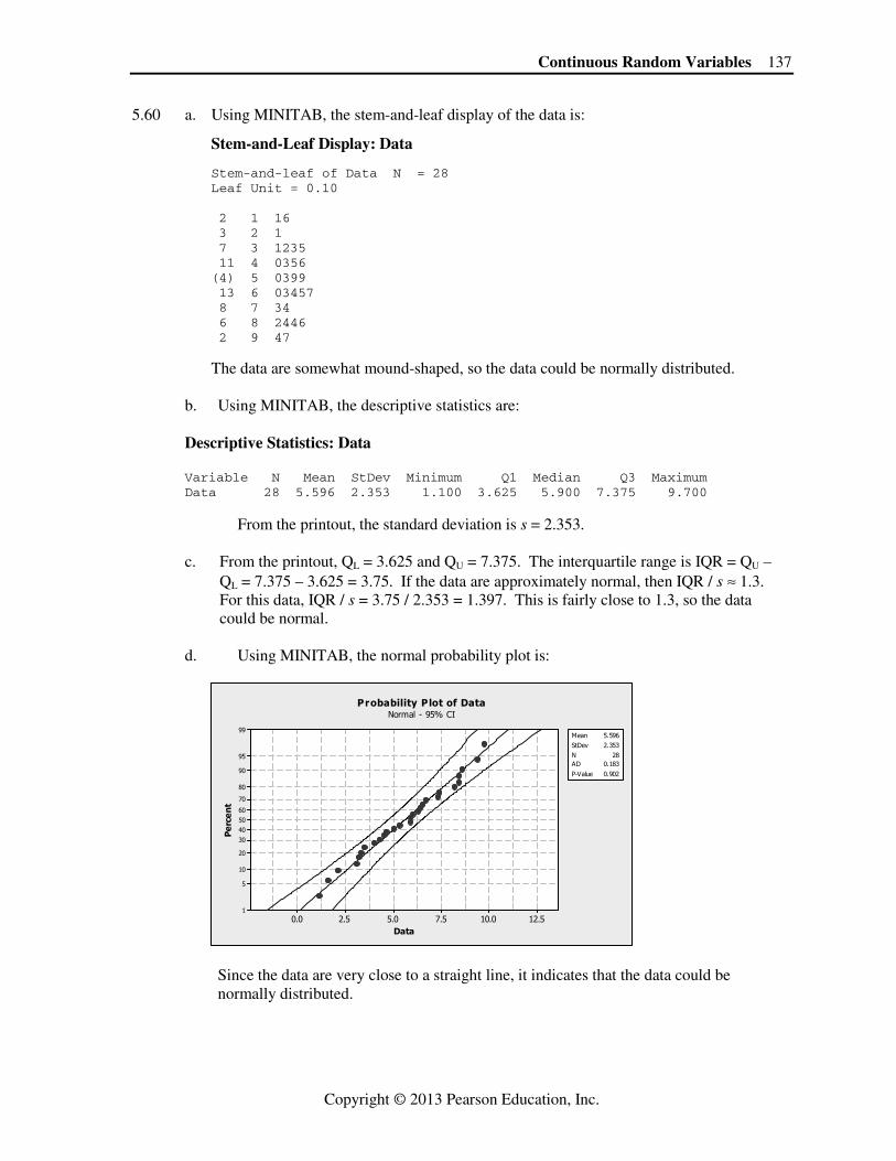
5.66 Using MINITAB, a histogram of the data with a normal curve drawn on the graph is:
S c o r e
Fre
qu
en
cy
35302520151050
50
40
30
20
10
0
Me a n 12 .21
StD e v 6 .3 11N 7 34
Histo g ra m o f Sco reN orm a l
From the graph, the data appear to be close to mound-shaped, so the data may be approximately normal.
Continuous Random Variables 139
Copyright © 2013 Pearson Education, Inc.
5.68 Distance: To determine if the distribution of distances is approximately normal, we will run through the tests. Using MINITAB, the stem-and-leaf display is: Stem-and-Leaf Display: Distance Stem-and-leaf of Distance N = 40 Leaf Unit = 1.0 1 28 3 4 28 689 10 29 011144 (11) 29 55556778889 19 30 0000001112234 6 30 59 4 31 01 2 31 68
From the stem-and-leaf display, the data look to be mound-shaped. The data may be normal. Using MINITAB, the descriptive statistics are: Descriptive Statistics: Distance Variable N Mean StDev Minimum Q1 Median Q3 Maximum Distance 40 298.95 7.53 283.20 294.60 299.05 302.00 318.90
The interval 298.95 7.53 (291.42, 306.48)x s± ⇒ ± ⇒ contains 28 of the 40 observations.
The proportion is 28 / 40 = .70. This is very close to the .68 from the Empirical Rule. The interval 2 298.95 2(7.53) 298.95 15.06 (283.89, 314.01)x s± ⇒ ± ⇒ ± ⇒ contains 37
of the 40 observations. The proportion is 37 / 40 = .925. This is somewhat smaller than the .95 from the Empirical Rule.
The interval 3 298.95 3(7.53) 298.95 22.59 (276.36, 321.54)x s± ⇒ ± ⇒ ± ⇒ contains 40
of the 40 observations. The proportion is 40 / 40 = 1.00. This is very close to the .997 from the Empirical Rule. Thus, it appears that the data may be normal.
The lower quartile is QL = 294.60 and the upper quartile is QU = 302. The interquartile range
is IQR = QU – QL = 302 – 294.60 = 7.4. From the printout, s = 7.53. IQR / s = 7.4 / 7.53 = .983. This is somewhat less than the 1.3 that we would expect if the data were normal. Thus, there is evidence that the data may not be normal.
140 Chapter 5
Copyright © 2013 Pearson Education, Inc.
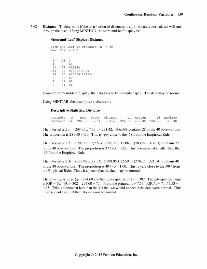
Using MINITAB, the normal probability plot is:
Distance
Pe
rce
nt
320310300290280
99
95
90
80
70
60
50
40
30
20
10
5
1
Mean
0.174
299.0StDev 7.525
N 40AD 0.521P-Value
Probability Plot of DistanceNormal - 95% C I
The data are very close to a straight line. Thus, it appears that the data may be normal. From 3 of the 4 indicators, it appears that the distances come from an approximate normal
distribution. Accuracy: To determine if the distribution of accuracies is approximately normal, we will
run through the tests. Using MINITAB, the stem-and-leaf display is: Stem-and-Leaf Display: Accuracy Stem-and-leaf of Accuracy N = 40 Leaf Unit = 1.0 1 4 5 1 4 1 4 2 5 0 2 5 3 5 4 7 5 6777 11 5 8999 20 6 000001111 20 6 2223333333 10 6 4 9 6 6667 5 6 899 2 7 0 1 7 3
From the stem-and-leaf display, the data look to be skewed to the left. The data may not be normal.
Continuous Random Variables 141
Copyright © 2013 Pearson Education, Inc.
Using MINITAB, the descriptive statistics are: Descriptive Statistics: Accuracy Variable N Mean StDev Minimum Q1 Median Q3 Maximum Accuracy 40 61.970 5.226 45.400 59.400 61.950 64.075 73.000
The interval 61.970 5.226 (56.744, 67.196)x s± ⇒ ± ⇒ contains 30 of the 40 observations.
The proportion is 30 / 40 = .75. This is somewhat larger than the .68 from the Empirical Rule.
The interval 2 61.970 2(5.226) 61.970 10.452 (51.518, 72.422)x s± ⇒ ± ⇒ ± ⇒ contains 37
of the 40 observations. The proportion is 37 / 40 = .925. This is somewhat smaller than the .95 from the Empirical Rule.
The interval 3 61.970 3(5.226) 61.970 15.678 (46.292, 77.648)x s± ⇒ ± ⇒ ± ⇒ contains 39
of the 40 observations. The proportion is 39 / 40 = .975. This is somewhat smaller than the .997 from the Empirical Rule. Thus, it appears that the data may not be normal.
The lower quartile is QL = 59.400 and the upper quartile is QU = 64.075. The interquartile
range is IQR = QU – QL = 64.075 – 59.400 = 4.675. From the printout, s = 5.226. IQR / s = 4.675 / 5.226 = .895. This is less than the 1.3 that we would expect if the data were normal. Thus, there is evidence that the data may not be normal.
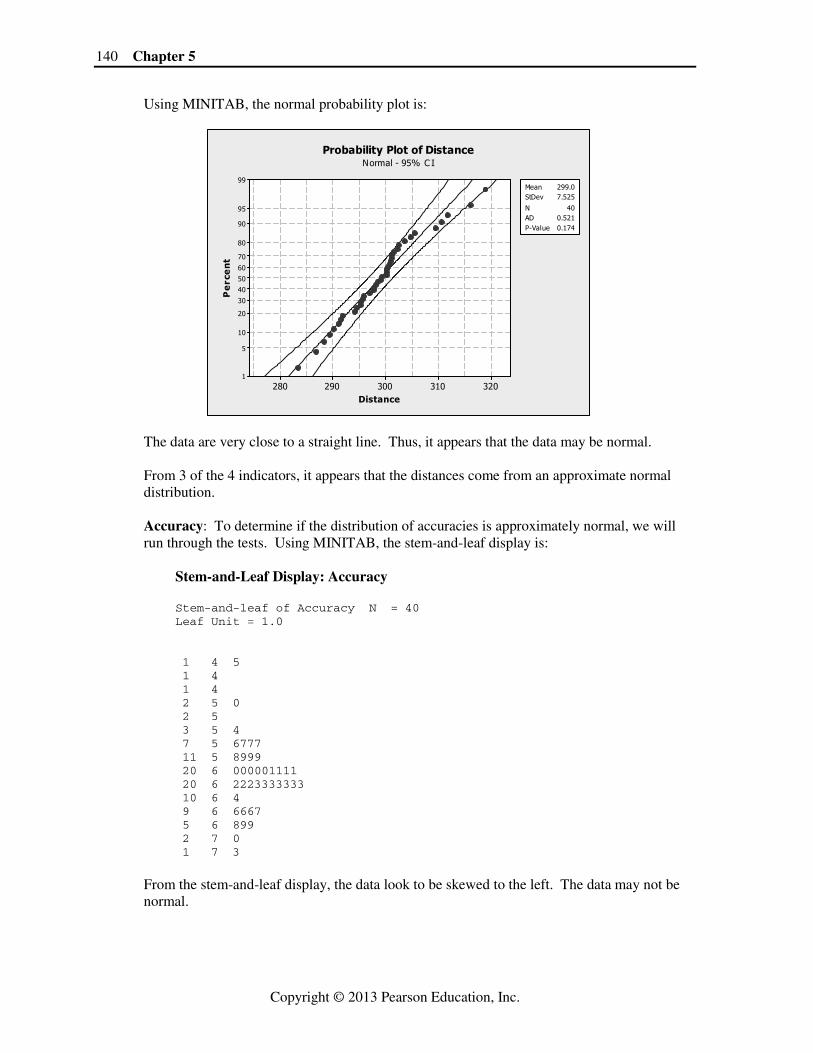
Using MINITAB, the normal probability plot is:
A ccuracy
Pe
rce
nt
8075706560555045
99
95
90
80
70
60
50
40
30
20
10
5
1
Mean
0.111
61.97StDev 5.226
N 40AD 0.601P-Value
Probability Plot of AccuracyNormal - 95% C I
The data are not real close to a straight line. Thus, it appears that the data may not be normal. From the 4 indicators, it appears that the accuracy values do not come from an approximate
normal distribution.
142 Chapter 5
Copyright © 2013 Pearson Education, Inc.
Index: To determine if the distribution of driving performance index scores is approximately normal, we will run through the tests. Using MINITAB, the stem-and-leaf display is: Stem-and-Leaf Display: ZSUM Stem-and-leaf of ZSUM N = 40 Leaf Unit = 0.10 1 1 1 8 1 2233333 18 1 4444445555 (4) 1 7777 18 1 8899 14 2 0 13 2 22222 8 2 5 7 2 77 5 2 8 4 3 1 3 3 2 2 3 45
From the stem-and-leaf display, the data look to be skewed to the right. The data may not be normal. Using MINITAB, the descriptive statistics are: Descriptive Statistics: ZSUM Variable N Mean StDev Minimum Q1 Median Q3 Maximum ZSUM 40 1.927 0.660 1.170 1.400 1.755 2.218 3.580
The interval 1.927 .660 (1.267, 2.587)x s± ⇒ ± ⇒ contains 30 of the 40 observations. The proportion is 30 / 40 = .75. This is somewhat larger than the .68 from the Empirical Rule. The interval 2 1.927 2(.660) 1.927 1.320 (.607, 3.247)x s± ⇒ ± ⇒ ± ⇒ contains 37 of the
40 observations. The proportion is 37 / 40 = .925. This is somewhat smaller than the .95 from the Empirical Rule.
The interval 3 1.927 3(.660) 1.927 1.98 ( .053, 3.907)x s± ⇒ ± ⇒ ± ⇒ − contains 40 of the
40 observations. The proportion is 40 / 40 = 1.000. This is slightly larger than the .997 from the Empirical Rule. Thus, it appears that the data may not be normal.
The lower quartile is QL = 1.4 and the upper quartile is QU = 2.218. The interquartile range is
IQR = QU – QL = 2.218 – 1.4 = .818. From the printout, s = .66. IQR / s = .818 / .66 = 1.24. This is fairly close to the 1.3 that we would expect if the data were normal. Thus, there is evidence that the data may be normal.
Continuous Random Variables 143
Copyright © 2013 Pearson Education, Inc.
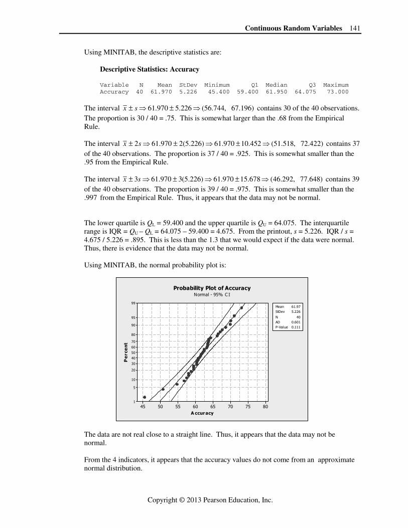
Using MINITAB, the normal probability plot is:
ZSUM
Pe
rce
nt
43210
99
95
90
80
70
60
50
40
30
20
10
5
1
Mean
<0.005
1.927StDev 0.6602
N 40AD 1.758P-Value
Probability Plot of ZSUMNormal - 95% C I
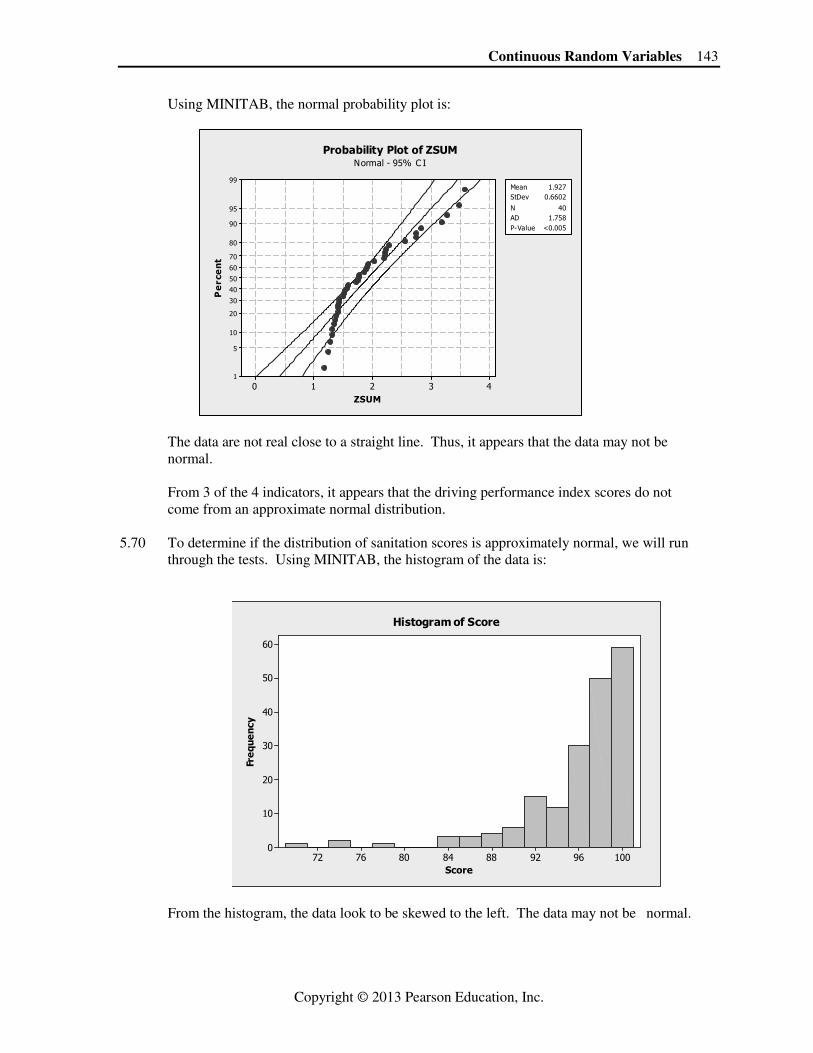
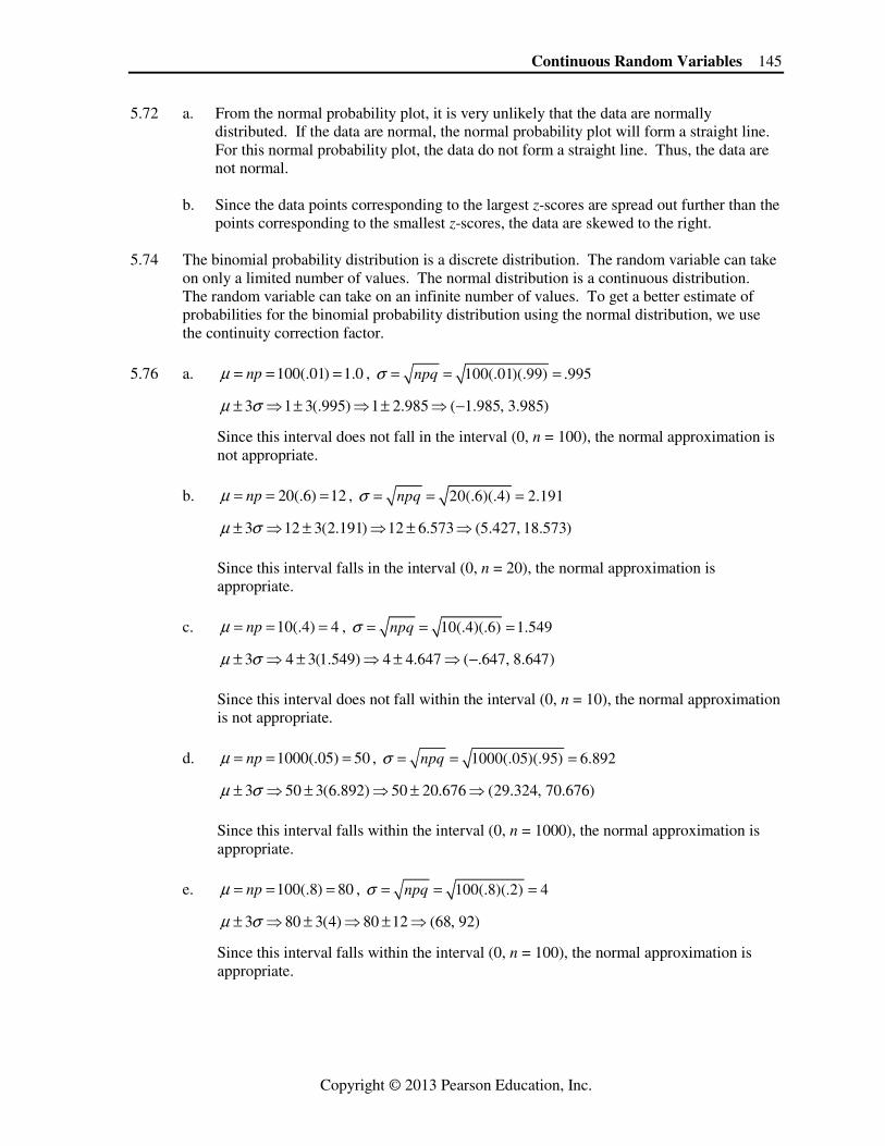
The data are not real close to a straight line. Thus, it appears that the data may not be normal. From 3 of the 4 indicators, it appears that the driving performance index scores do not come from an approximate normal distribution. 5.70 To determine if the distribution of sanitation scores is approximately normal, we will run through the tests. Using MINITAB, the histogram of the data is:
Score
Freq
uenc
y
10096928884807672
60
50
40
30
20
10
0
Histogram of Score
From the histogram, the data look to be skewed to the left. The data may not be normal.

144 Chapter 5
Copyright © 2013 Pearson Education, Inc.
Using MINITAB, the descriptive statistics are: Descriptive Statistics: Score
Variable N Mean StDev Minimum Q1 Median Q3 Maximum Score 186 95.699 4.963 69.000 94.000 97.000 99.000 100.000
The interval 95.70 4.96 (90.74, 100.66)x s± ⇒ ± ⇒ contains 166 of the 186 observations.
The proportion is 166 / 186 = .892. This is much larger than the .68 from the Empirical Rule. The interval 2 95.70 2(4.96) 95.70 9.92 (85.78, 105.62)x s± ⇒ ± ⇒ ± ⇒ contains 179 of the
186 observations. The proportion is 179 / 186 = .962. This is somewhat larger than the .95 from the Empirical Rule.
The interval 3 95.70 3(4.96) 95.70 14.88 (80.82, 110.58)x s± ⇒ ± ⇒ ± ⇒ contains 182 of
the 186 observations. The proportion is 182 / 186 = .978. This is somewhat smaller than the .997 from the Empirical Rule. Thus, it appears that the data may not be normal.
The lower quartile is QL = 94 and the upper quartile is QU = 99. The interquartile range is
IQR = QU – QL = 99 – 94 = 5. From the printout, s = 4.963. IQR / s = 5 / 4.963 = 1.007. This is not particularly close to the 1.3 that we would expect if the data were normal. Thus, there is evidence that the data may not be normal.
Using MINITAB, the normal probability plot is:
Score
Perc
ent
110100908070
99.9
99
9590
80706050403020
10
5
1
0.1
Mean
<0.005
95.70StDev 4.963N 186AD 11.663P-Value
Probability Plot of ScoreNormal - 95% CI
The data are not real close to a straight line. Thus, it appears that the data may not be normal. From the 4 indicators, it appears that the sanitation scores do not come from an approximate
normal distribution.
Continuous Random Variables 145
Copyright © 2013 Pearson Education, Inc.
5.72 a. From the normal probability plot, it is very unlikely that the data are normally distributed. If the data are normal, the normal probability plot will form a straight line. For this normal probability plot, the data do not form a straight line. Thus, the data are not normal.
b. Since the data points corresponding to the largest z-scores are spread out further than the
points corresponding to the smallest z-scores, the data are skewed to the right. 5.74 The binomial probability distribution is a discrete distribution. The random variable can take
on only a limited number of values. The normal distribution is a continuous distribution. The random variable can take on an infinite number of values. To get a better estimate of probabilities for the binomial probability distribution using the normal distribution, we use the continuity correction factor.
5.76 a. 100(.01) 1.0npµ = = = , 100(.01)(.99) .995npqσ = = = 3 1 3(.995) 1 2.985 ( 1.985, 3.985)µ σ± ⇒ ± ⇒ ± ⇒ − Since this interval does not fall in the interval (0, n = 100), the normal approximation is
not appropriate.
b. 20(.6) 12npµ = = = , 20(.6)(.4) 2.191npqσ = = = 3 12 3(2.191) 12 6.573 (5.427, 18.573)µ σ± ⇒ ± ⇒ ± ⇒ Since this interval falls in the interval (0, n = 20), the normal approximation is
appropriate. c. 10(.4) 4npµ = = = , 10(.4)(.6) 1.549npqσ = = = 3 4 3(1.549) 4 4.647 ( .647, 8.647)µ σ± ⇒ ± ⇒ ± ⇒ − Since this interval does not fall within the interval (0, n = 10), the normal approximation
is not appropriate.
d. 1000(.05) 50npµ = = = , 1000(.05)(.95) 6.892npqσ = = = 3 50 3(6.892) 50 20.676 (29.324, 70.676)µ σ± ⇒ ± ⇒ ± ⇒ Since this interval falls within the interval (0, n = 1000), the normal approximation is
appropriate. e. 100(.8) 80npµ = = = , 100(.8)(.2) 4npqσ = = = 3 80 3(4) 80 12 (68, 92)µ σ± ⇒ ± ⇒ ± ⇒ Since this interval falls within the interval (0, n = 100), the normal approximation is
appropriate.
146 Chapter 5
Copyright © 2013 Pearson Education, Inc.
f. 35(.7) 24.5npµ = = = , 35(.7)(.3) 2.711npqσ = = = 3 24.5 3(2.711) 24.5 8.133 (16.367, 32.633)µ σ± ⇒ ± ⇒ ± ⇒ Since this interval falls within the interval (0, n = 35), the normal approximation is
appropriate.
5.78 1000(.5) 500npµ = = = , 1000(.5)(.5) 15.811npqσ = = = a. Using the normal approximation,
(500 .5) 500
( 500) ( .03) .5 .0120 .488015.811
P x P z P z+ −⎛ ⎞> ≈ > = > = − =⎜ ⎟
⎝ ⎠
(from Table IV, Appendix A)
b. (490 .5) 500 (500 .5) 500
(490 500)15.811 15.811
P x P z− − − −⎛ ⎞≤ < ≈ ≤ <⎜ ⎟
⎝ ⎠
( .66 .03) .2454 .0120 .2334P z= − ≤ < − = − = (from Table IV, Appendix A)
c. (500 .5) 500
( 550) ( 3.19) .5 .5 015.811
P x P z P z+ −⎛ ⎞> ≈ > = > ≈ − =⎜ ⎟
⎝ ⎠
(from Table IV, Appendix A)
5.80 a. For this exercise n = 500 and p = .5.
500(.5) 250npµ = = = and 500(.5)(.5) 125 11.1803npqσ = = = =
b. 240 250
.8911.1803
xz
µσ− −= = = −
c. 270 250
1.7911.1803
xz
µσ− −= = =
d. 3 250 3(11.1803) 250 33.5409 (216.4591, 283.5409)µ σ± ⇒ ± ⇒ ± ⇒
Since the above is completely contained in the interval 0 to 500, the normal approximation is valid.
( ) ( )240 .5 250 270 .5 250
(240 270)11.1803 11.1803
P x P z⎛ ⎞+ − − −
< < = < <⎜ ⎟⎜ ⎟⎝ ⎠
( .85 1.74) .3023 .4591 .7614P z= − < < = + = (Using Table IV, Appendix A)
Continuous Random Variables 147
Copyright © 2013 Pearson Education, Inc.
5.82 a. Let x = number of patients who experience serious post-laser vision problems in 100,000 trials. Then x is a binomial random variable with n = 100,000 and p =.01.
( ) 100,000(.01) 1000E x npµ= = = = . b. 2( ) 100, 000(.01)(.99) 990V x npqσ= = = =
c. 950 1000 50
1.5931.4643990
xz
µσ− − −= = = = −
d. 3 1000 3(31.4643) 1000 94.3929 (905.6071, 1 094 3929), .µ σ± ⇒ ± ⇒ ± ⇒ Since the
interval lies in the range 0 to 100,000, we can use the normal approximation to approximate the binomial probability.
(950 .5) 1000
( 950) ( 1.60) .5 .4452 .054831.4643
P x P z P z− −⎛ ⎞< = < = < − = − =⎜ ⎟
⎝ ⎠
(Using Table IV, Appendix A) 5.84 a. ( ) ( )1000 .32 320E x npµ = = = = . This is the same value that was found in Exercise 4.66 a.
b. 1000(.32)(1 .32) 217.6 14.751npqσ = = − = = This is the same value that was
found in Exercise 4.66 b.
c. 200.5 320
8.1014.751
xz
µσ− −= = = −
d. 3 320 3(14.751) 320 44.253 (275.474, 364.253)µ σ± ⇒ ± ⇒ ± ⇒
Since the above is completely contained in the interval 0 to 1000, the normal approximation is valid.
200.5 320
( 200) ( 8.10) .5 .5 014.751
P x P z P z−⎛ ⎞≤ ≈ ≤ = ≤ − ≈ − =⎜ ⎟
⎝ ⎠
(Using Table IV, Appendix A) 5.86 For this exercise, n = 100 and p = .4. 100(.4) 40npµ = = = and 100(.4)(.6) 24 4.899npqσ = = = =
3 40 3(4.899) 40 14.697 (25.303, 54.697)µ σ± ⇒ ± ⇒ ± ⇒
Since the above is completely contained in the interval 0 to 100, the normal approximation is valid.
(50 .5) 40
( 50) ( 1.94) .5 .4738 .97384.899
P x P z P z− −⎛ ⎞< = < = < = + =⎜ ⎟
⎝ ⎠
(Using Table IV, Appendix A)
148 Chapter 5
Copyright © 2013 Pearson Education, Inc.
5.88 a. Let x = number of abused women in a sample of 150. The random variable x is a binomial random variable with n = 150 and p = 1/3. Thus, for the normal approximation,
150(1 / 3) 50npµ = = = and 150(1 / 3)(2 / 3) 5.7735npqσ = = =
3 50 3(5.7735) 50 17.3205 (32.6795, 67.3205)µ σ± ⇒ ± ⇒ ± ⇒
Since this interval lies in the range from 0 to n = 150, the normal approximation is appropriate.
(75 .5) 50
( 75) ( 4.42) .5 .5 05.7735
P x P z P z+ −⎛ ⎞> ≈ > = > ≈ − =⎜ ⎟
⎝ ⎠
(Using Table IV, Appendix A.)
b. (50 .5) 50
( 50) ( .09) .5 .0359 .46415.7735
P x P z P z− −⎛ ⎞< ≈ < = < − ≈ − =⎜ ⎟
⎝ ⎠
c. (30 .5) 50
( 30) ( 3.55) .5 .5 05.7735
P x P z P z− −⎛ ⎞< ≈ < = < − ≈ − =⎜ ⎟
⎝ ⎠
Since the probability of seeing fewer than 30 abused women in a sample of 150 is so small (p ≈ 0), it would be very unlikely to see this event.
5.90 a. Let x equal the percentage of body fat in American men. The random variable x is a
normal random variable with µ = 15 and σ = 2. P(Man is obese) ( 20)P x= ≥
20 15
2
( 2.5)
.5000 .4938 .0062
P z
P z
−⎛ ⎞≈ ≥⎜ ⎟⎝ ⎠
= ≥= − =
(Using Table IV in Appendix A.) Let y equal the number of men in the U.S. Army who are obese in a sample of 10,000.
The random variable y is a binomial random variable with n = 10,000 and p = .0062.
3 3 10,000(.0062) 3 10,000(.0062)(1 .0062)
62 3(7.85) (38.45, 85.55)
np npqµ σ± ⇒ ± ⇒ ± −⇒ ± ⇒
Since the interval does lie in the range 0 to 10,000, we can use the normal
approximation to approximate the probability.
(50 .5) 62
( 50)7.85
P x P z− −⎛ ⎞< ≈ <⎜ ⎟
⎝ ⎠
( 1.59)
.5000 .4441 .0559
P z≈ < −= − =
(Using Table IV in Appendix A.) b. The probability of finding less than 50 obese Army men in a sample of 10,000 is .0559.
Therefore, the probability of finding only 30 would even be smaller. Thus, it looks like the Army has successfully reduced the percentage of obese men since this did occur.

Continuous Random Variables 149
Copyright © 2013 Pearson Education, Inc.
5.92 Let x = number of patients who wait more than 30 minutes. Then x is a binomial random variable with n = 150 and p = .5.
a. ( )150 .5 75, 150(.5)(.5) 6.124np npqµ σ= = = = = =
(75 .5) 75
( 75) ( .08) .5 .0319 .46816.124
P x P z P z+ −⎛ ⎞> ≈ > = > = − =⎜ ⎟
⎝ ⎠
(from Table IV, Appendix A)
b. (85 .5) 75
( 85) ( 1.71) .5 .4564 .04366.124
P x P z P z+ −⎛ ⎞> ≈ > = > = − =⎜ ⎟
⎝ ⎠
(from Table IV, Appendix A)
c. (60 .5) 75 (90 .5) 75
(60 90)6.124 6.124
( 2.37 2.37) .4911 .4911 .9822
P x P z
P z
+ − − −⎛ ⎞< < ≈ < <⎜ ⎟⎝ ⎠
= − < < = + =
(from Table IV, Appendix A) 5.94 The exponential distribution is often called the waiting time distribution. 5.96 a. If θ = 1, a = 1, then / 1 .367879ae eθ− −= = b. If θ = 1, a = 2.5, then / 2.5 .082085ae eθ− −= = c. If θ = .4, a = 3, then / 7.5 .000553ae eθ− −= = d. If θ = .2, a = .3, then / 1.5 .223130ae eθ− −= = 5.98 a. 4/2.5 1.6( 4) 1 ( 4) 1 1 1 .201897 .798103P x P x e e− −≤ = − > = − = − = − = b. 5/2.5 2( 5) .135335P x e e− −> = = = c. 2/2.5 .8( 2) 1 ( 2) 1 1 1 .449329 .550671P x P x e e− −≤ = − > = − = − = − = d. 3/2.5 1.2( 3) .301194P x e e− −> = = =
5.100 With 2θ = , /21( ) ( 0)
2xf x e x−= >
2µ σ θ= = = a. 3 2 3(2) 2 6 ( 4, 8)µ σ± ⇒ ± ⇒ ± ⇒ − Since 3µ σ− lies below 0, find the probability that x is more than 3 8µ σ+ = . 8/2 4( 8) .018316P x e e− −> = = = (using Table V in Appendix A)
150 Chapter 5
Copyright © 2013 Pearson Education, Inc.
b. 2 2 2(2) 2 4 ( 2, 6)µ σ± ⇒ ± ⇒ ± ⇒ − Since 2µ σ− lies below 0, find the probability that x is between 0 and 6. 6/2 3( 6) 1 ( 6) 1 1 1 .049787 .950213P x P x e e− −< = − ≥ = − = − = − = (using Table V in Appendix A) c. .5 2 .5(2) 2 1 (1, 3)µ σ± ⇒ ± ⇒ ± ⇒
1/2 3/2 .5 1.5
(1 3) ( 1) ( 3)
.606531 .223130
.383401
P x P x P x
e e e e− − − −
< < = > − >
= − = −= −=
(using Table V in Appendix A) 5.102 a. Let x = time until the first critical part failure. Then x has an exponential distribution
with .1θ = . 1/.1 10( 1) .000045P x e e− −≥ = = = (using Table V, Appendix A)
b. 30 minutes = .5 hours. .5/.1 5( .5) 1 ( .5) 1 1 1 .006738 .993262P x P x e e− −< = − ≥ = − = − = − =
(using Table V, Appendix A)
5.104 a. Let x = time between component failures. Then x has an exponential distribution with 1000.θ =
1200/1000 1500/1000 1.2 1.5
(1200 1500) ( 1200) ( 1500)
.301194 .223130 .078064
P x P x P x
e e e e− − − −
< < = > − >
= − = − = − =
(using Table V, Appendix A)
b. 1200/1000 1.2( 1200) .301194P x e e− −≥ = = = (using Table V, Appendix A)
c. (1200 1500 .078064
( 1500 | 1200) .259182( 1200) .301194
P xP x x
P x
≤ << ≥ = = =≥
5.106 a. Let x = anthropogenic fragmentation index. Then x has an exponential distribution with 23µ θ= = .
20 40
23 23(20 40) ( 20) ( 40) .419134 .1756730 .243461P x P x P x e e− −< < = > − ≥ = − = − =
b. 50
23( 50) 1 ( 50) 1 1 .113732 .886268P x P x e−< = − ≥ = − = − =
Continuous Random Variables 151
Copyright © 2013 Pearson Education, Inc.
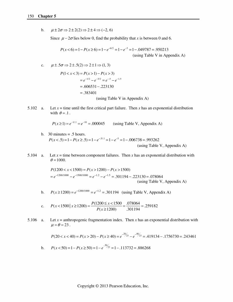
c. Using MINITAB, the histogram of the natural fragmentation index is:
F-Natural
Freq
uenc
y
3224168
10
8
6
4
2
0
Histogram of F-Natural
An exponential distribution is skewed to the right. This histogram does not have that shape. 5.108 a. Let x = life length of CD-ROM. Then x has an exponential distribution with 25,000θ = .
/ 25,000( ) ( ) tR t P x t e−= > = b. 8,760/25,000 .3504(8,760) ( 8,760) .704406R P x e e− −= > = = =
c. S(t) = probability that at least one of two drives has a length exceeding t hours = 1 – probability that neither has a length exceeding t hours
1 2 1 2
/25,000 /25,000
/25,000 /12,500 /25,000 /12,500
1 ( ) ( ) 1 [1 ( )][1 ( )]
1 [1 ][1 ]
1 [1 2 ] 2
t t
t t t t
P x t P x t P x t P x t
e e
e e e e
− −
− − − −
= − ≤ ≤ = − − > − >
= − − −
= − − + = −
d. 8,760/25,000 8,760/12,500(8,760) 2 2(.704406) .496188
1.408812 .496188 .912624
S e e− −= − = −= − =
e. The probability in part d is greater than that in part b. We would expect this. The
probability that at least one of the systems lasts longer than 8,760 hours would be greater than the probability that only one system lasts longer than 8,760 hours.
152 Chapter 5
Copyright © 2013 Pearson Education, Inc.
5.110 Let x = life length of a product. Then x has an exponential distribution with µ θ= .
/( ) .5
ln(.5) .6931
.6931( )
mP x m e
m
m
θ
θθ
−> = =−
⇒ = = −
⇒ =
The median is equal to .6931 times the mean of the distribution. 5.112 a. A score on an IQ test probably follows a normal distribution.
b. Time waiting in line at a supermarket checkout counter probably follows an exponential distribution.
c. The amount of liquid dispensed into a can of soda probably follows a normal
distribution. d. The difference between SAT scores for tests taken at two different times probably
follows a uniform distribution.
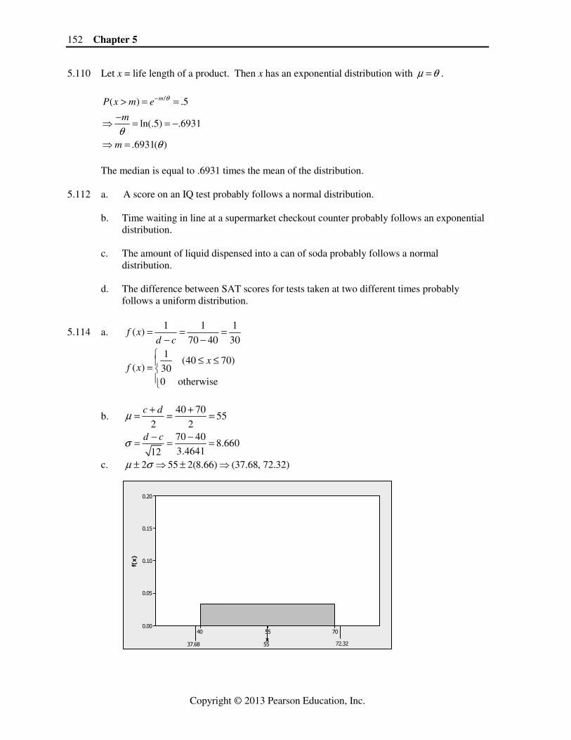
5.114 a. 1 1 1
( )70 40 30
f xd c
= = =− −
1
(40 70)( ) 30
0 otherwise
xf x
⎧ ≤ ≤⎪= ⎨⎪⎩
b. 40 70
552 2
c dµ + += = =
70 40
8.6603.464112
d cσ − −= = =
c. 2 55 2(8.66) (37.68, 72.32)µ σ± ⇒ ± ⇒
x
f(x)
705540
0.20
0.15
0.10
0.05
0.00
5537.68 72.32
Continuous Random Variables 153
Copyright © 2013 Pearson Education, Inc.
d. 1
( 45) (45 30) .16730
P x ≤ = − =
e. 1
( 58) (70 58) .430
P x ≥ = − =
f. ( 100) 1P x ≤ = , since this range includes all possible values of x. g. 55 8.66 (46.34, 63.66)µ σ± ⇒ ± ⇒
1
( ) (46.34 63.66) (63.66 46.34) .57730
P x P xµ σ µ σ− < < + = < < = − =
h. 1
( 60) (70 60) .33330
P x > = − =
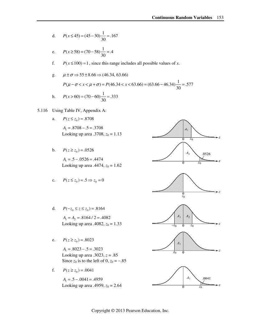
5.116 Using Table IV, Appendix A: a. 0( ) .8708P z z≤ = 1 .8708 .5 .3708A = − = Looking up area .3708, z0 = 1.13 b. 0( ) .0526P z z≥ = 1 .5 .0526 .4474A = − = Looking up area .4474, z0 = 1.62
c. 0 0( ) .5 0P z z z≤ = ⇒ =
d. 0 0( ) .8164P z z z− ≤ ≤ = 1 2 .8164 / 2 .4082A A= = = Looking up area .4082, z0 = 1.33 e. 0( ) .8023P z z≥ = 1 .8023 .5 .3023A = − = Looking up area .3023, z = .85 Since z0 is to the left of 0, z0 = −.85
f. 0( ) .0041P z z≥ = 1 .5 .0041 .4959A = − = Looking up area .4959, z0 = 2.64
154 Chapter 5
Copyright © 2013 Pearson Education, Inc.
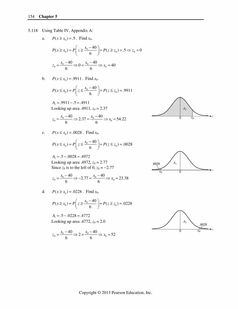
5.118 Using Table IV, Appendix A: a. 0( ) .5P x x≥ = . Find x0.
00 0 0
40( ) ( ) .5 0
6
xP x x P z P z z z
−⎛ ⎞≥ = ≥ = ≥ = ⇒ =⎜ ⎟⎝ ⎠
0 00 0
40 400 40
6 6
x xz x
− −= ⇒ = ⇒ =
b. 0( ) .9911P x x≤ = . Find x0.
00 0
40( ) ( ) .9911
6
xP x x P z P z z
−⎛ ⎞≤ = ≤ = ≤ =⎜ ⎟⎝ ⎠
1 .9911 .5 .4911A = − = Looking up area .4911, z0 = 2.37
0 00 0
40 402.37 54.22
6 6
x xz x
− −= ⇒ = ⇒ =
c. 0( ) .0028P x x≤ = . Find x0.
00 0
40( ) ( ) .0028
6
xP x x P z P z z
−⎛ ⎞≤ = ≤ = ≤ =⎜ ⎟⎝ ⎠
1 .5 .0028 .4972A = − = Looking up area .4972, z0 = 2.77 Since z0 is to the left of 0, z0 = −2.77
0 00 0
40 402.77 23.38
6 6
x xz x
− −= ⇒ − = ⇒ =
d. 0( ) .0228P x x≥ = . Find x0.
00 0
40( ) ( ) .0228
6
xP x x P z P z z
−⎛ ⎞≥ = ≥ = ≥ =⎜ ⎟⎝ ⎠
1 .5 .0228 .4772A = − = Looking up area .4772, z0 = 2.0
0 00 0
40 402 52
6 6
x xz x
− −= ⇒ = ⇒ =
Continuous Random Variables 155
Copyright © 2013 Pearson Education, Inc.
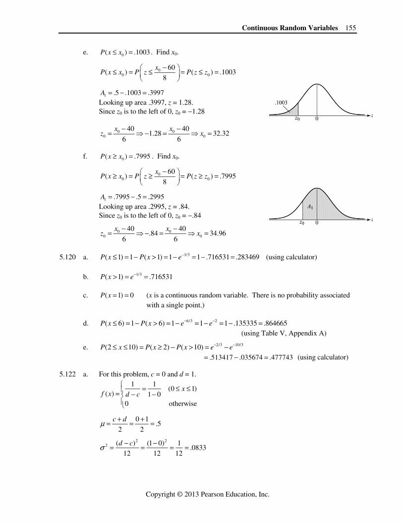
e. 0( ) .1003P x x≤ = . Find x0.
00 0
60( ) ( ) .1003
8
xP x x P z P z z
−⎛ ⎞≤ = ≤ = ≤ =⎜ ⎟⎝ ⎠
1 .5 .1003 .3997A = − = Looking up area .3997, z = 1.28. Since z0 is to the left of 0, z0 = −1.28
0 00 0
40 401.28 32.32
6 6
x xz x
− −= ⇒ − = ⇒ =
f. 0( ) .7995P x x≥ = . Find x0.
00 0
60( ) ( ) .7995
8
xP x x P z P z z
−⎛ ⎞≥ = ≥ = ≥ =⎜ ⎟⎝ ⎠
1 .7995 .5 .2995A = − = Looking up area .2995, z = .84. Since z0 is to the left of 0, z0 = −.84
0 00 0
40 40.84 34.96
6 6
x xz x
− −= ⇒ − = ⇒ =
5.120 a. 1/3( 1) 1 ( 1) 1 1 .716531 .283469P x P x e−≤ = − > = − = − = (using calculator) b. 1/3( 1) .716531P x e−> = = c. ( 1) 0P x = = (x is a continuous random variable. There is no probability associated
with a single point.) d. 6/3 2( 6) 1 ( 6) 1 1 1 .135335 .864665P x P x e e− −≤ = − > = − = − = − = (using Table V, Appendix A) e. 2/3 10/3(2 10) ( 2) ( 10)P x P x P x e e− −≤ ≤ = ≥ − > = − .513417 .035674 .477743= − = (using calculator) 5.122 a. For this problem, c = 0 and d = 1.
1 1
(0 1)( ) 1 0
0 otherwise
xf x d c
⎧ = ≤ ≤⎪= − −⎨⎪⎩
0 1
.52 2
c dµ + += = =
2 2
2 ( ) (1 0) 1.0833
12 12 12
d cσ − −= = = =
156 Chapter 5
Copyright © 2013 Pearson Education, Inc.
b. (.2 .4) (.4 .2)(1) .2P x< < = − = c. ( .995) (1 .995)(1) .005P x > = − = . Since the probability of observing a trajectory greater
than .995 is so small, we would not expect to see a trajectory exceeding .995. 5.124 a. Let x = change in SAT-MATH score. Using Table IV, Appendix A,
50 19
( 50) ( .48) .5 .1844 .315665
P x P z P z−⎛ ⎞≥ = ≥ = ≥ = − =⎜ ⎟
⎝ ⎠.
b. Let x = change in SAT-VERBAL score. Using Table IV, Appendix A,
50 7
( 50) ( .88) .5 .3106 .189449
P x P z P z−⎛ ⎞≥ = ≥ = ≥ = − =⎜ ⎟
⎝ ⎠.
5.126 a. Let x = weight of captured fish. Using Table IV, Appendix A,
1,000 1,050 1,400 1,050
(1,000 1,400) ( .13 .93)375 375
.0517 .3238 .3755
P x P z P z− −⎛ ⎞< < = < < = − < <⎜ ⎟
⎝ ⎠= + =
b. 800 1,050 1, 000 1,050
(800 1, 000) ( .67 .13)375 375
.2486 .0517 .1969
P x P z P z− −⎛ ⎞< < = < < = − < < −⎜ ⎟
⎝ ⎠= − =
c. 1,750 1,050
( 1,750) ( 1.87) .5 .4693 .9693375
P x P z P z−⎛ ⎞< = < = < = + =⎜ ⎟
⎝ ⎠
d. 500 1,050
( 500) ( 1.47) .5 .4292 .9292375
P x P z P z−⎛ ⎞> = > = > − = + =⎜ ⎟
⎝ ⎠
e. 1,050 1,050
( ) .95 .95 1.645375 375
616.875 1,050 1,666.875
o oo
o o
x xP x x P z z
x x
− −⎛ ⎞< = ⇒ < = ⇒ = =⎜ ⎟⎝ ⎠
⇒ = − ⇒ =
Continuous Random Variables 157
Copyright © 2013 Pearson Education, Inc.
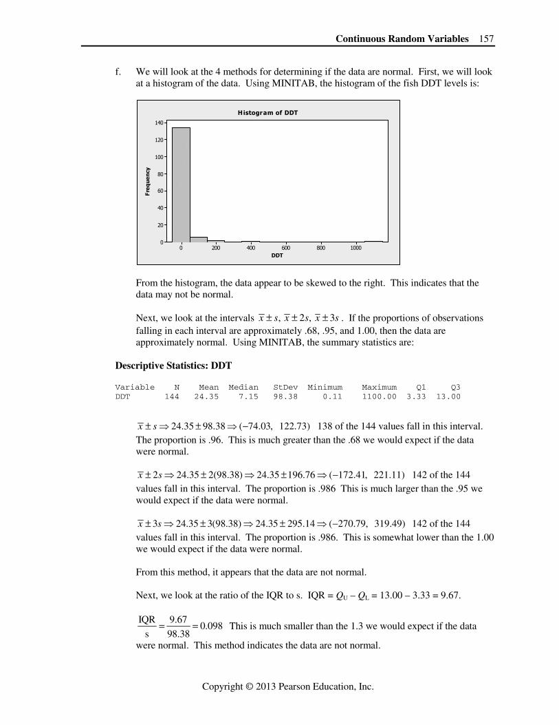
f. We will look at the 4 methods for determining if the data are normal. First, we will look at a histogram of the data. Using MINITAB, the histogram of the fish DDT levels is:
DDT
Freq
uenc
y
10008006004002000
140
120
100
80
60
40
20
0
Histogram of DDT
From the histogram, the data appear to be skewed to the right. This indicates that the data may not be normal. Next, we look at the intervals , 2 , 3x s x s x s± ± ± . If the proportions of observations falling in each interval are approximately .68, .95, and 1.00, then the data are approximately normal. Using MINITAB, the summary statistics are:
Descriptive Statistics: DDT
Variable N Mean Median StDev Minimum Maximum Q1 Q3 DDT 144 24.35 7.15 98.38 0.11 1100.00 3.33 13.00
24.35 98.38 ( 74.03, 122.73)x s± ⇒ ± ⇒ − 138 of the 144 values fall in this interval. The proportion is .96. This is much greater than the .68 we would expect if the data were normal.
2 24.35 2(98.38) 24.35 196.76 ( 172.41, 221.11)x s± ⇒ ± ⇒ ± ⇒ − 142 of the 144 values fall in this interval. The proportion is .986 This is much larger than the .95 we would expect if the data were normal.
3 24.35 3(98.38) 24.35 295.14 ( 270.79, 319.49)x s± ⇒ ± ⇒ ± ⇒ − 142 of the 144 values fall in this interval. The proportion is .986. This is somewhat lower than the 1.00 we would expect if the data were normal. From this method, it appears that the data are not normal. Next, we look at the ratio of the IQR to s. IQR = QU – QL = 13.00 – 3.33 = 9.67. IQR 9.67
0.098s 98.38
= = This is much smaller than the 1.3 we would expect if the data
were normal. This method indicates the data are not normal.

158 Chapter 5
Copyright © 2013 Pearson Education, Inc.
Finally, using MINITAB, the normal probability plot is:
DDT
Perc
ent
125010007505002500-250-500
99.9
99
95
90
80706050403020
10
5
1
0.1
Mean
<0.005
24.36StDev 98.38N 144AD 38.851P-Value
Probability P lot of DDTNormal - 95% CI
Since the data do not form a straight line, the data are not normal. From the 4 different methods, all indications are that the fish DDT level data are not normal.
5.128 a. ( )200 .5 100npµ = = =
b. 200(.5)(.5) 50 7.071npqσ = = = =
c. 110 100
1.417.071
xz
µσ− −= = =
d. (110 .5) 100
( 110) ( 1.48) .5 .4306 .93067.071
P x P z P z+ −⎛ ⎞≤ ≈ ≤ = ≤ = + =⎜ ⎟
⎝ ⎠
(Using Table IV, Appendix A) 5.130 Let x = interarrival time between patients. Then x is an exponential random variable with a
mean of 4 minutes. a. ( 1) 1 ( 1)P x P x< = − ≥
1/4 .251 1 1 .778801 .221199e e− −= − = − = − = (Using Table V, Appendix A) b. Assuming that the interarrival times are independent, P(next 4 interarrival times are all less than 1 minute) 4 4{ ( 1)} .221199 .002394P x= < = = c. 10/4 2.5( 10) .082085P x e e− −> = = =

Continuous Random Variables 159
Copyright © 2013 Pearson Education, Inc.
5.132 a. For layer 2, 10 50
302 2
c dµ + += = = thousand dollars.
b. For layer 6, 500 1000
7502 2
c dµ + += = = thousand dollars.
c. Let x = marine loss for layer 2. 50 30 20
( 30) .550 10 40
P x−> = = =−
d. Let x = marine loss for layer 6. 800 750 50
(750 800) .11000 500 500
P x−< < = = =−
5.134 Let x1 = score on the blue exam. Then x1 is approximately normal with 1 53%µ = and 1 15%σ = .
1
20 53( 20%) ( 2.20) .5 .4861 .0139
15P x P z P z
−⎛ ⎞< = < = < − = − =⎜ ⎟⎝ ⎠
Let x2 = score on the red exam. Then x2 is approximately normal with 2 39%µ = and 2 12%σ = .
2
20 39( 20%) ( 1.58) .5 .4429 .0571
12P x P z P z
−⎛ ⎞< = < = < − = − =⎜ ⎟⎝ ⎠
Since the probability of scoring below 20% on the red exam is greater than the probability of scoring below 20% on the blue exam, it is more likely that a student will score below 20% on
the red exam. 5.136 a. Let x = gestation length. Using Table IV, Appendix A,
( ) 275.5 280 276.5 280275.5 276.5 ( .23 .18)
20 20
.0910 .0714 .0196
P x P z P z− −⎛ ⎞< < = < < = − < < −⎜ ⎟
⎝ ⎠= − =
b. Using Table IV, Appendix A,
( ) 258.5 280 259.5 280258.5 259.5 ( 1.08 1.03)
20 20
.3599 .3485 .0114
P x P z P z− −⎛ ⎞< < = < < = − < < −⎜ ⎟
⎝ ⎠= − =
c. Using Table IV, Appendix A,
( ) 254.5 280 255.5 280254.5 255.5 ( 1.28 1.23)
20 20
.3997 .3907 .0090
P x P z P z− −⎛ ⎞< < = < < = − < < −⎜ ⎟
⎝ ⎠= − =

160 Chapter 5
Copyright © 2013 Pearson Education, Inc.
d. If births are independent, then P(baby 1 is 4 days early ∩ baby 2 is 21 days early ∩ baby 3 is 25 days early) = P(baby 1 is 4 days early) P(baby 2 is 21 days early) P(baby 3 is 25 days early)
= .0196(.0114)(.0090) = .00000201. 5.138 Let x = number of parents who condone spanking in 150 trials. Then x is a binomial random
variable with n = 150 and p = .6. 150(.6) 90npµ = = = 150(.6)(.4) 36 6npqσ = = = =
(20 .5) 90
( 20) ( 11.58) 06
P x P z P z+ −⎛ ⎞≤ ≈ ≤ = ≤ − ≈⎜ ⎟
⎝ ⎠
If, in fact, 60% of parents with young children condone spanking, the probability of seeing no
more than 20 out of 150 parent clients who condone spanking is essentially 0. Thus, the claim made by the psychologist is either incorrect or the 60% figure is too high.
5.140 a. Using Table IV, Appendix A, with 450µ = and 40σ = ,
( ) 00
450.10
40
xP x x P z
−⎛ ⎞< = ⇒ <⎜ ⎟⎝ ⎠
0( ) .10P z z= < =
1 .5 .10 .4000A = − = Looking up the area .4000 in Table IV gives z0 = 1.28. Since z0 is to the left of 0,
z0 = −1.28.
00 0
4501.28 40( 1.28) 450 398.8
40
xz x
−= − = ⇒ = − + = seconds.
5.142 a. Using Table IV, Appendix A, with 24.1µ = and 6.30σ = ,
20 24.1
( 20) ( .65) .2422 .5 .74226.30
P x P z P z−⎛ ⎞≥ = ≥ = ≥ − = + =⎜ ⎟
⎝ ⎠
b. 10.5 24.1
( 10.5) ( 2.16) .5 .4846 .01546.30
P x P z P z−⎛ ⎞≤ = ≤ = ≤ − = − =⎜ ⎟
⎝ ⎠ c. No. The probability of having a cardiac patient who participates regularly in sports or
exercise with a maximum oxygen uptake of 10.5 or smaller is very small (p = .0154). It is very unlikely that this patient participates regularly in sports or exercise.
Continuous Random Variables 161
Copyright © 2013 Pearson Education, Inc.
5.144 a. Using Table IV, Appendix A, with 99µ = and 4.3σ = ,
( ) 00 0
99.99 ( ) .99
4.3
xP x x P z P z z
−⎛ ⎞< = ⇒ < = < =⎜ ⎟⎝ ⎠
1 .99 .5 .4900A = − = Looking up the area .4900 in Table IV gives z0 = 2.33. Since z0 is to the right of 0,
z0 = 2.33.
00 0
992.33 4.3(2.33) 99 109.019
4.3
xz x
−= = ⇒ = + =
5.146 With 30µ θ= = , /301( ) ( 0)
30xf x e x−= >
P(outbreaks within 6 years) ( 6)P x= ≤
6/30 .21 ( 6) 1 1 1 .818731 .181269P x e e− −= − > = − = − = − = (using Table V, Appendix A) 5.148 a. Let x1 = repair time for machine 1. Then x1 has an exponential distribution with
1 1µ = hour. 1/1 1
1( 1) .367879P x e e− −> = = = (using Table V, Appendix A) b. Let x2 = repair time for machine 2. Then x2 has an exponential distribution with
2 2µ = hours. 1/2 .5
2( 1) .606531P x e e− −> = = = (using Table V, Appendix A) c. Let x3 = repair time for machine 3. Then x3 has an exponential distribution with
3 .5µ = hours. 1/.5 2
3( 1) .135335P x e e− −> = = = (using Table V, Appendix A) Since the mean repair time for machine 4 is the same as for machine 3,
4 3( 1) ( 1) .135335P x P x> = > = . d. The only way that the repair time for the entire system will not exceed 1 hour is if all
four machines are repaired in less than 1 hour. Thus, the probability that the repair time for the entire system exceeds 1 hour is:
P(Repair time entire system exceeds 1 hour)
1 2 3 4
1 2 3 4
1 [( 1) ( 1) ( 1) ( 1)]
1 ( 1) ( 1) ( 1) ( 1)
1 (1 .367879)(1 .606531)(1 .135335)(1 .135335)
1 (.632121)(.393469)(.864665)(.864665) 1 .185954 .814046
P x x x x
P x P x P x P x
= − ≤ ∩ ≤ ∩ ≤ ∩ ≤= − ≤ ≤ ≤ ≤= − − − − −= − = − =

162 Chapter 5
Copyright © 2013 Pearson Education, Inc.
5.150 a. Define x = the number of serious accidents per month. Then x has a Poisson distribution with 2λ = . If we define y = the time between adjacent serious accidents, then y has an exponential distribution with 1 / 1 / 2µ λ= = . If an accident occurs today, the probability that the next serious accident will not occur during the next month is:
1(2) 2( 1) .135335P y e e− −> = = = Alternatively, we could solve the problem in terms of the random variable x by noting
that the probability that the next serious accident will not occur during the next month is the same as the probability that the number of serious accident next month is zero, i.e.,
( ) ( )2 0
221 0 .135335
0!
eP y P x e
−−> = = = = =
b. ( 1) 1 ( 1) 1 .406 .594P x P x> = − ≤ = − = (Using Table III in Appendix A with 2λ = ) 5.152 Let x = weight of corn chip bag. Then x is a normal random variable with 10.5µ = and .25σ = .
10 10.5
( 10) ( 2.00) .4772 .5000 .9772.25
P x P z P z−⎛ ⎞> = > = > − = + =⎜ ⎟
⎝ ⎠
(Using Table IV, Appendix A) Let y = number of corn chip bags with more than 10 ounces. Then x is a binomial random variable with n = 1,500 and p = .9772. 1500(.9772) 1465.8npµ = = = and 1500(.9772)(.0228) 5.781npqσ = = =
97% of the 1500 chip bags is 1455
(1455 .5) 1465.8
( 1455) ( 1.78) .5 .4625 .03755.781
P y P z P z+ −⎛ ⎞≤ = ≤ = ≤ − = − =⎜ ⎟
⎝ ⎠