Chapter Eight

The Material Balance Equation (MBE)

The material balance equation (MBE) has long been recognized as one of the basic

tools of reservoir engineers for interpreting and predicting reservoir performance. The

MBE, when properly applied, can be used to:

• Estimate initial hydrocarbon volumes in place.

• Predict future reservoir performance.

• Predict ultimate hydrocarbon recovery under various types of primary driving

mechanisms

The equation is structured to simply keep inventory of all materials entering,

leaving, and accumulating in the reservoir. The concept of the material balance

equation was presented by Schilthuis in 1941. In its simplest form, the equation can be

written on a volumetric basis as:

Initial volume =volume remaining +volume removed

Since oil, gas, and water are present in petroleum reservoirs, the mate-rial balance

equation can be expressed for the total fluids or for any one of the fluids present.

Before deriving the material balance, it is convenient to denote certain terms by

symbols for brevity. The symbols used conform where possible to the standard

nomenclature adopted by the Society of Petroleum Engineers.

Several of the material balance calculations require the total pore volume (P.V) as

expressed in terms of the initial oil volume N and the volume of the gas cap. The

expression for the total pore volume can be derived by conveniently introducing the

parameter m into the relation-ship as follows: Defining the ratio m as:

Or

(8.1)

where Swi=initial water saturation

N=initial oil-in-place, STB

P.V=total pore volume, bbl

m=ratio of initial gas-cap gas reservoir volume to

initial reservoir oil volume, bbl/bbl

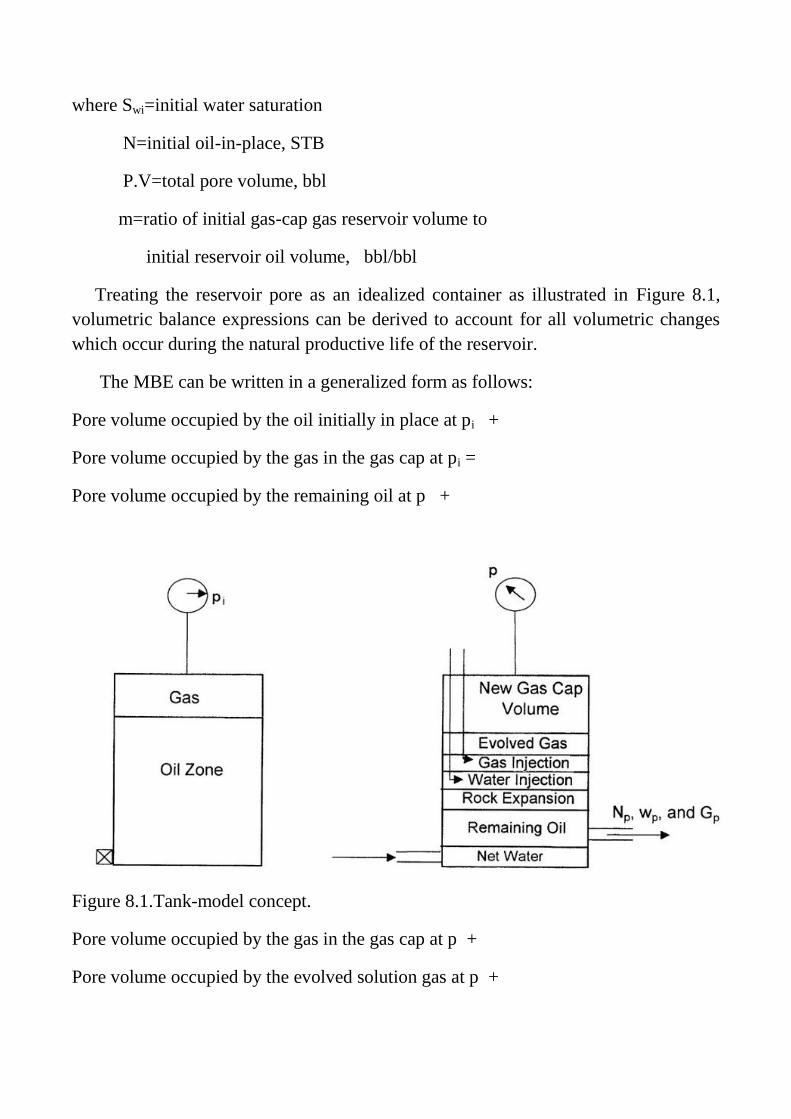
Treating the reservoir pore as an idealized container as illustrated in Figure 8.1,

volumetric balance expressions can be derived to account for all volumetric changes

which occur during the natural productive life of the reservoir.

The MBE can be written in a generalized form as follows:

Pore volume occupied by the oil initially in place at pi +

Pore volume occupied by the gas in the gas cap at pi =

Pore volume occupied by the remaining oil at p +

Figure 8.1.Tank-model concept.

Pore volume occupied by the gas in the gas cap at p +

Pore volume occupied by the evolved solution gas at p +

Pore volume occupied by the net water influx at p +

Change in pore volume due to connate-water expansion and pore

volume reduction due to rock expansion +

Pore volume occupied by the injected gas at p +

Pore volume occupied by the injected water at p (8-2)

The above nine terms composing the MBE can be separately deter-mined from the

hydrocarbon PVT and rock properties, as follows:

Pore Volume Occupied by the Oil Initially in Place

Volume occupied by initial oil-in-place =N Boi (8-3)

where N=oil initially in place, STB

Boi=oil formation volume factor at initial reservoir pressure pi, bbl/STB

Pore Volume Occupied by the Gas in the Gas Cap

Volume of gas cap =m N Boi (8-4)

where m is a dimensionless parameter and defined as the ratio of gas-cap volume to

the oil zone volume.

Pore Volume Occupied by the Remaining Oil

Volume of the remaining oil =(N −Np) Bo (8-5)

where Np=cumulative oil production, STB

Bo=oil formation volume factor at reservoir pressure p, bbl/STB

Pore Volume Occupied by the Gas Cap at Reservoir Pressure p

As the reservoir pressure drops to a new level p, the gas in the gas cap expands and

occupies a larger volume. Assuming no gas is produced from the gas cap during the

pressure decline, the new volume of the gas cap can be determined as:

(8-6)

where Bgi=gas formation volume factor at initial reservoir pressure, bbl/scf

Bg=current gas formation volume factor, bbl/scf

Pore Volume Occupied by the Evolved Solution Gas

This volumetric term can be determined by applying the following material balance

on the solution gas:

Or

(8.7)

Pore Volume Occupied by the Net Water Influx

net water influx =We−Wp Bw (8-8)

where We=cumulative water influx, bbl

Wp=cumulative water produced, STB

Bw=water formation volume factor, bbl/STB

Change in Pore Volume Due to Initial Water and Rock Expansion

The component describing the reduction in the hydrocarbon pore volume due to the

expansion of initial (connate) water and the reservoir rock cannot be neglected for an

under saturated-oil reservoir. The water compressibility cw and rock compressibility cf

are generally of the same order of magnitude as the compressibility of the oil. The

effect of these two components, however, can be generally neglected for the gas-cap-

drive reservoir or when the reservoir pressure drops below the bubble-point pressure.

The compressibility coefficient c, which describes the changes in the volume

(expansion) of the fluid or material with changing pressure, is given by:

where ΔV represents the net changes or expansion of the material as a result of

changes in the pressure. Therefore, the reduction in the pore volume due to the

expansion of the connate-water in the oil zone and the gas cap is given by:

Connate-water expansion =[(pore volume) Swi] cw Δp

Substituting for the pore volume (P.V) with Equation 8-1 gives:

(8.9)

Where Δp=change in reservoir pressure, (pi −p)

cw=water compressibility coefficient, psi−1

m=ratio of the volume of the gas-cap gas to the reservoir oil volume, bbl/bbl

Similarly, the reduction in the pore volume due to the expansion of the reservoir

rock is given by:

(8.10)

Combining the expansions of the connate-water and formation as represented by

Equations 8-9 and 8-10 gives:

(8.11)

Pore Volume Occupied by the Injection Gas and Water

Assuming that Ginj volumes of gas and Winj volumes of water have been injected

for pressure maintenance, the total pore volume occupied by the two injected fluids is

given by:

Total volume =Ginj Bginj+Winj Bw (8-12)

where Ginj =cumulative gas injected, scf

Bginj =injected gas formation volume factor, bbl/scf

Winj =cumulative water injected, STB

Bw=water formation volume factor, bbl/STB

Combining Equations 8-3 through 8-12 with Equation 8-2 and rearranging gives:

(8-13)

The cumulative gas produced Gp can be expressed in terms of the cumulative gas-

oil ratio Rp and cumulative oil produced Np by:

Gp=Rp Np (8-14)

Combining Equation 8-14 with Equation 8-13 gives:

(8.15)

The above relationship is referred to as the material balance equation (MBE). A

more convenient form of the MBE can be determined by introducing the concept of

the total (two-phase) formation volume factor Bt into the equation. This oil PVT

property is defined as:

(8.16)

Introducing Bt into Equation 8-15 and assuming, for the sake of simplicity, no water or

gas injection gives:

(8-17)

where Swi=initial water saturation

Rp=cumulative produced gas-oil ratio, scf/STB

Δp=change in the volumetric average reservoir pressure, psi

In a combination-drive reservoir where all the driving mechanisms are

simultaneously present, it is of practical interest to determine the relative magnitude of

each of the driving mechanisms and its contribution to the production.

Rearranging Equation 8-17 gives:

(8-18)

with the parameter A as defined by:

(8.19)

Equation 8-18 can be abbreviated and expressed as:

DDI +SDI +WDI +EDI =1.0 (8-20)

where DDI=depletion-drive index

SDI=segregation (gas-cap)-drive index

WDI=water-drive index

EDI=expansion (rock and liquid)-drive index

The four terms of the left-hand side of Equation 8-20 represent the major primary

driving mechanisms by which oil may be recovered from oil reservoirs. As presented

earlier in this chapter, these driving forces are:

a.Depletion Drive.

Depletion drive is the oil recovery mechanism wherein the production of the oil

from its reservoir rock is achieved by the expansion of the original oil volume with all

its original dissolved gas. This driving mechanism is represented mathematically by

the first term of Equation 8-18 or:

DDI =N (Bt −Bti)/A (8-21)

where DDI is termed the depletion-drive index.

b.Segregation Drive.

Segregation drive (gas-cap drive) is the mechanism wherein the displacement of

oil from the formation is accomplished by the expansion of the original free gas cap.

This driving force is described by the second term of Equation 8-18, or:

SDI =[N m Bti (Bg−Bgi)/Bgi]/A (8-22)

where SDI is termed the segregation-drive index.

c.Water Drive.

Water drive is the mechanism wherein the displacement of the oil is accomplished

by the net encroachment of water into the oil zone. This mechanism is represented by

the third term of Equation 8-18 or:

WDI =(We−Wp Bw)/A (8-23)

where WDI is termed the water-drive index.

d.Expansion Drive.

For under saturated-oil reservoirs with no water influx, the principal source of

energy is a result of the rock and fluid expansion. Where all the other three driving

mechanisms are contributing to the production of oil and gas from the reservoir, the

contribution of the rock and fluid expansion to the oil recovery is too small and

essentially negligible and can be ignored.

Cole (1969) pointed out that since the sum of the driving indexes is equal to one, it

follows that if the magnitude of one of the index terms is reduced, then one or both of

the remaining terms must be correspondingly increased. An effective water drive will

usually result in maximum recovery from the reservoir. Therefore, if possible, the

reservoir should be operated to yield a maximum water-drive index and minimum

values for the depletion-drive index and the gas-cap-drive index. Maximum advantage

should be taken of the most efficient drive available, and where the water drive is too

weak to provide an effective displacing force, it may be possible to utilize the

displacing energy of the gas cap. In any event, the depletion-drive index should be

maintained as low as possible at all times, as this is normally the most inefficient

driving force available.

Equation 8-20 can be solved at any time to determine the magnitude of the various

driving indexes. The forces displacing the oil and gas from the reservoir are subject to

change from time to time and for this reason Equation 8-20 should be solved

periodically to determine whether there has been any change in the driving indexes.

Changes in fluid withdrawal rates are primarily responsible for changes in the driving

indexes. For example, reducing the oil-producing rate could result in an increased

water-drive index and a correspondingly reduced depletion-drive index in a reservoir

containing a weak water drive. Also, by shutting in wells producing large quantities of

water, the water-drive index could be increased, as the net water influx (gross water

influx minus water production) is the important factor.

When the reservoir has a very weak water drive but a fairly large gas cap, the most

efficient reservoir producing mechanism may be the gas cap, in which case a large

gas-cap-drive index is desirable. Theoretically, recovery by gas-cap drive is

independent of producing rate, as the gas is readily expansible. Low vertical

permeability could limit the rate of expansion of the gas cap, in which case the gas-

cap-drive index would be rate sensitive. Also, gas coning into producing wells will

reduce the effectiveness of the gas-cap expansion due to the production of free gas.

Gas coning is usually a rate sensitive phenomenon; the higher the producing rates, the

greater the amount of coning.

An important factor in determining the effectiveness of a gas-cap drive is the

degree of conservation of the gas-cap gas. As a practical matter, it will often be

impossible, because of royalty owners or lease agreements, to completely eliminate

gas-cap gas production. Where free gas is being produced, the gas-cap-drive index can

often be markedly increased by shutting in high gas-oil ratio wells and, if possible,

transferring their allowables to other low gas-oil ratio wells.

Figure 8.2 shows a set of plots that represent various driving indexes for a

combination-drive reservoir. At point A, some of the structurally low wells are

reworked to reduce water production. This resulted in an effective increase in the

water-drive index. At point B, work over operations are complete; water-, gas-, and

oil-producing rates are relatively stable; and the driving indexes show no change. At

point C, some of the wells which have been producing relatively large, but constant,

volumes of water are shut-in, which results in an increase in the water-drive index. At

the same time, some of the up structure, high gas-oil ratio wells have been shut-in and

their allowables transferred to wells lower on the structure producing with normal gas-

oil ratios. At point D, gas is being returned to the reservoir, and the gas-cap-drive

index is exhibiting a decided increase.

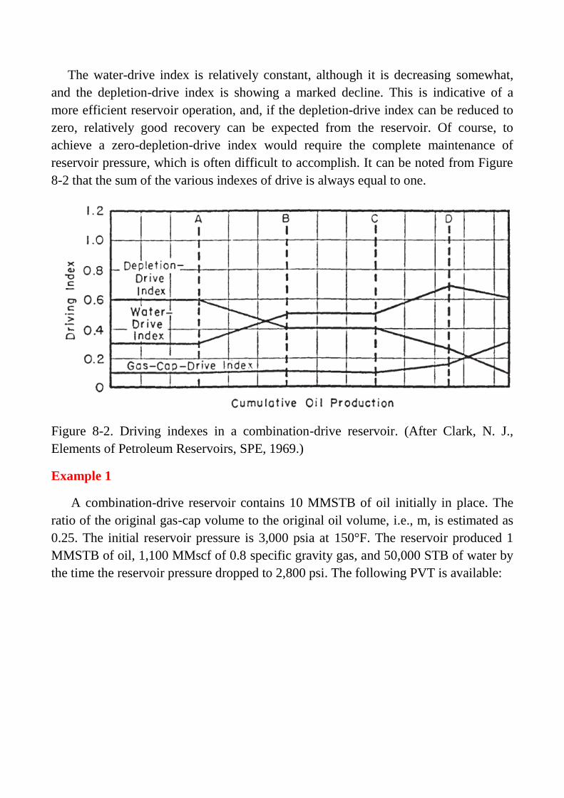
The water-drive index is relatively constant, although it is decreasing somewhat,

and the depletion-drive index is showing a marked decline. This is indicative of a

more efficient reservoir operation, and, if the depletion-drive index can be reduced to

zero, relatively good recovery can be expected from the reservoir. Of course, to

achieve a zero-depletion-drive index would require the complete maintenance of

reservoir pressure, which is often difficult to accomplish. It can be noted from Figure

8-2 that the sum of the various indexes of drive is always equal to one.

Figure 8-2. Driving indexes in a combination-drive reservoir. (After Clark, N. J.,

Elements of Petroleum Reservoirs, SPE, 1969.)

Example 1

A combination-drive reservoir contains 10 MMSTB of oil initially in place. The

ratio of the original gas-cap volume to the original oil volume, i.e., m, is estimated as

0.25. The initial reservoir pressure is 3,000 psia at 150°F. The reservoir produced 1

MMSTB of oil, 1,100 MMscf of 0.8 specific gravity gas, and 50,000 STB of water by

the time the reservoir pressure dropped to 2,800 psi. The following PVT is available:

Calculate:

a. Cumulative water influx

b. Net water influx

c. Primary driving indexes at 2,800 psi

Solution

Because the reservoir contains a gas cap, the rock and fluid expansion can be

neglected, i.e., set cf and cw=0. For illustration purposes, how-ever, the rock and fluid

expansion term will be included in the calculations.

Part A. Cumulative water influx

Step 1.Calculate cumulative gas-oil ratio Rp:

Step 2.Arrange Equation 8-17 to solve for We:

Neglecting the rock and fluid expansion term, the cumulative water influx is 417,700

bbl.

Part B. Net water influx

Net water influx =We−Wp Bw=411,281 −50,000 =361,281 bbl

Part C. Primary recovery indexes

Step 1.Calculate the parameter A by using Equation 11-19:

A=106[1.655 +(1100 −1040) 0.00092] =1,710,000

Step 2.Calculate DDI, SDI, and WDI by applying Equations 8-21 through 8-23,

respectively:

These calculations show that the 43.85% of the recovery was obtained by

depletion drive, 34.65% by gas-cap drive, 21.12% by water drive, and only 0.38% by

connate-water and rock expansion. The results suggest that the expansion-drive index

(EDI) term can be neglected in the presence of a gas cap or when the reservoir

pressure drops below the bubble-point pressure. In high pore volume compressibility

reservoirs, such as chalks and unconsolidated sands, however, the energy contribution

of the rock and water expansion cannot be ignored even at high gas saturations.

Productivity equation

Productivity Index and IPR

A commonly used measure of the ability of the well to produce is the productivity

index. Defined by the symbol J, the productivity index is the ratio of the total liquid

flow rate to the pressure drawdown. For a water-free oil production, the productivity

index is given by:

(8.24)

The productivity index is generally measured during a production test on the well.

The well is shut-in until the static reservoir pressure is reached. The well is then

allowed to produce at a constant flow rate of Q and a stabilized bottom-hole flow

pressure of pwf. Since a stabilized pressure at surface does not necessarily indicate a

stabilized pwf, the bottom-hole flowing pressure should be recorded continuously from

the time the well is to flow. The productivity index is then calculated from Equation 8-

24.

It is important to note that the productivity index is a valid measure of the well

productivity potential only if the well is flowing at pseudo steady-state conditions.

Therefore, in order to accurately measure the productivity index of a well, it is

essential that the well is allowed to flow at a constant flow rate for a sufficient amount

of time to reach the pseudo steady-state as illustrated in Figure 8-3. The figure

indicates that during the transient flow period, the calculated values of the productivity

index will vary depending upon the time at which the measurements of pwf are made.

Figure 8-3.Productivity index during flow regimes.

The productivity index can be numerically calculated by recognizing that J must be

defined in terms of semisteady-state flow conditions. Recalling the following equation

for compressible Fluids:

then

(8.25)

The above equation is combined with Equation 8.24 to give:

(8.26)

The oil relative permeability concept can be conveniently introduced into Equation

8.26 to give:

(8.27)

Since most of the well life is spent in a flow regime that is approximating the

pseudosteady-state, the productivity index is a valuable methodology for predicting

the future performance of wells. Further, by monitoring the productivity index during

the life of a well, it is possible to determine if the well has become damaged due to

completion, workover, production, injection operations, or mechanical problems. If a

measured J has an unexpected decline, one of the indicated problems should be

investigated.

A comparison of productivity indices of different wells in the same reservoir

should also indicate some of the wells might have experienced unusual difficulties or

damage during completion. Since the productivity indices may vary from well to well

because of the variation in thickness of the reservoir, it is helpful to normalize the

indices by dividing each by the thickness of the well. This is defined as the specific

productivity index Js ,or:

(8.28)

Assuming that the well’s productivity index is constant, Equation 8.24 can be

rewritten as:

(8.29)

Where Δp=drawdown, psi

J=productivity index

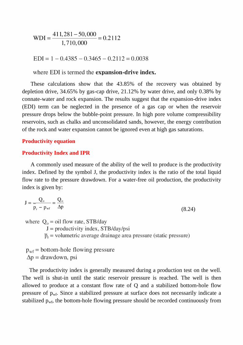
Equation 8.29 indicates that the relationship between Qo and Δp is a straight line

passing through the origin with a slope of J as shown in Figure 8.4.

Figure 8.4 Qo vs. Δp relationship.

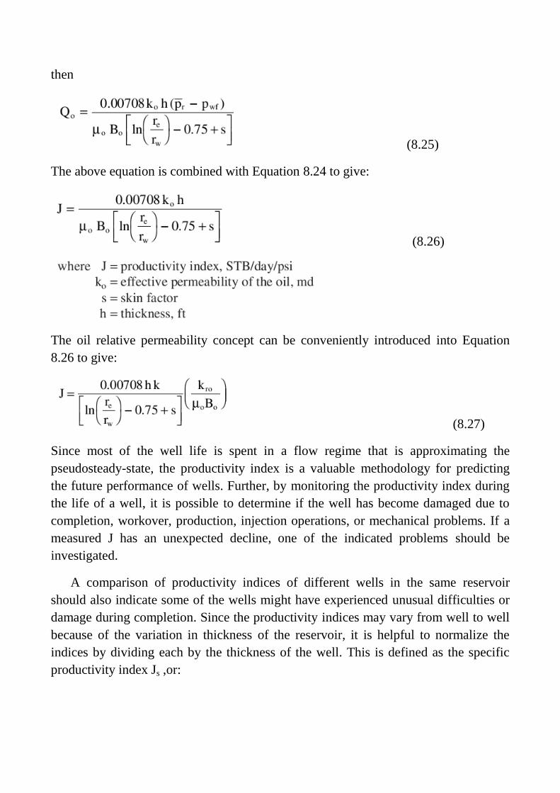
Alternatively, Equation 8.24 can be written as:

(8.30)

The above expression shows that the plot pwf against Qo is a straight line with a slope

of (−1/J) as shown schematically in Figure 8.5. This graphical representation of the

relationship that exists between the oil flow rate and bottom-hole flowing pressure is

called the inflow performance relationship and referred to as IPR. Several important

features of the straight-line IPR can be seen in Figure 8.5:

• When pwf equals average reservoir pressure, the flow rate is zero due to the absence

of any pressure drawdown.

• Maximum rate of flow occurs when pwf is zero. This maximum rate is called absolute

open flow and referred to as AOF. Although in practice this may not be a condition at

which the well can produce, it is a useful definition that has widespread applications in

the petroleum industry

Figure 8.5 IPR.

(e.g., comparing flow potential of different wells in the field). The AOF is then

calculated by:

•The slope of the straight line equals the reciprocal of the productivity index.

There are several empirical methods that are designed to generate the current and

future inflow performance relationships such as:

•Vogel’s method

•Wiggins’ method

•Standing’s method

•Fetkovich’s method

• The Klins-Clark method

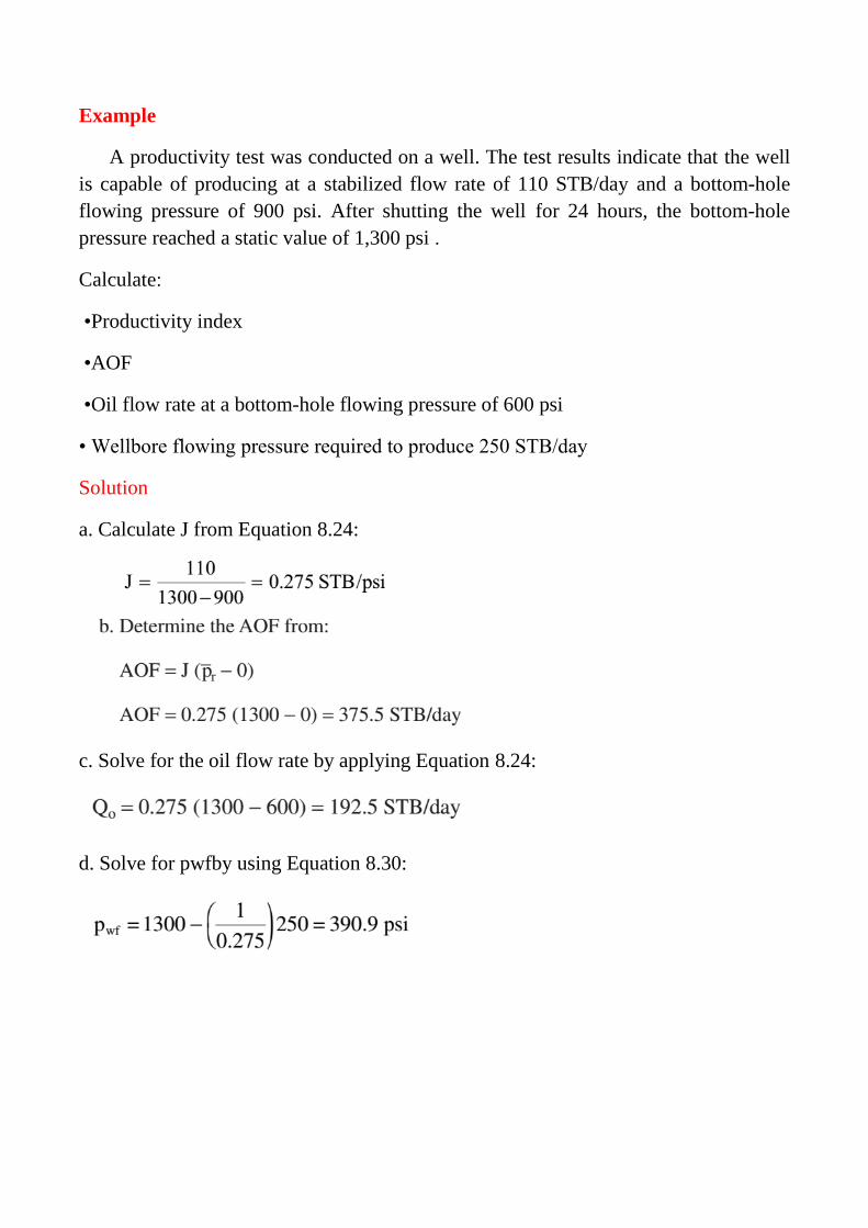
Example

A productivity test was conducted on a well. The test results indicate that the well

is capable of producing at a stabilized flow rate of 110 STB/day and a bottom-hole

flowing pressure of 900 psi. After shutting the well for 24 hours, the bottom-hole

pressure reached a static value of 1,300 psi .

Calculate:

•Productivity index

•AOF

•Oil flow rate at a bottom-hole flowing pressure of 600 psi

• Wellbore flowing pressure required to produce 250 STB/day

Solution

a. Calculate J from Equation 8.24:

c. Solve for the oil flow rate by applying Equation 8.24:

d. Solve for pwfby using Equation 8.30:

Fractional flow equation and buckley-Leverett equation.

The development of the fractional flow equation is attributed to Leverett (1941).

For two immiscible fluids, oil and water, the fractional flow of water, fw (or any

immiscible displacing fluid), is defined as the water flow rate divided by the total flow

rate, or:

(8.31)

where fw =fraction of water in the flowing stream, i.e., water cut , bbl/bbl

qt =total flow rate, bbl/day

qw =water flow rate, bbl/day

qo =oil flow rate, bbl/day

Consider the steady-state flow of two immiscible fluids (oil and water )through a

tilted-linear porous media as shown in Figure 8.6. Assuming a homogeneous system,

Darcy’s equation can be applied for each of the fluids:

(8.32)

(8.33)

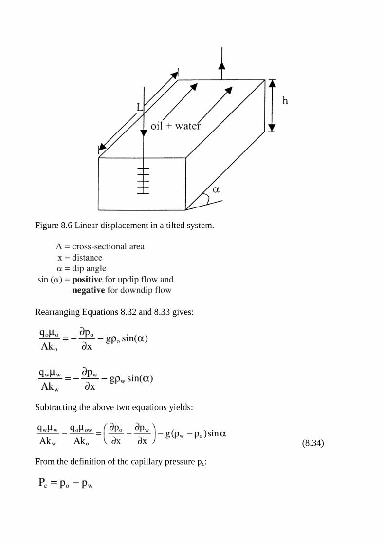
Figure 8.6 Linear displacement in a tilted system.

Rearranging Equations 8.32 and 8.33 gives:

Subtracting the above two equations yields:

(8.34)

From the definition of the capillary pressure pc:

Differentiating the above expression with respect to the distance x gives:

(8.35)

Combining Equation 8.35 with 8.36 gives:

(8.36)

where Δρ=ρw�ρo. From the water cut equation, i.e., Equation 8.31:

(8.37)

Replacing qo and qw in Equation 8.36 with those of Equation 8.37 gives:

In field units, the above equation can be expressed as:

(8.38)

Noting that the relative permeability ratios kro/krw =ko/kw and , for two-phase flow,

the total flow rate qt are essentially equal to the water-injection rate, i.e., iw=qt,

Equation 8.38 can be expressed more conveniently in terms of kro/krw and iw as:

(8.39)

The fractional flow equation as expressed by the above relationship suggests that

for a given rock-fluid system, all the terms in the equation are defined by the

characteristics of the reservoir, except:

•water-injection rate, iw

•water viscosity, μw

•direction of the flow, i.e., up dip or down dip injection

Equation 8.39 can be expressed in a more generalized form to describe the fractional

flow of any displacement fluid as:

(8.40)

where the subscript D refers to the displacement fluid and Δρ is defined as:

For example, when the displacing fluid is immiscible gas, then:

(8.41)

The effect of capillary pressure is usually neglected because the capillary pressure

gradient is generally small and, thus, Equations 8.39 and 8.41 are reduced to:

(8.42)

and

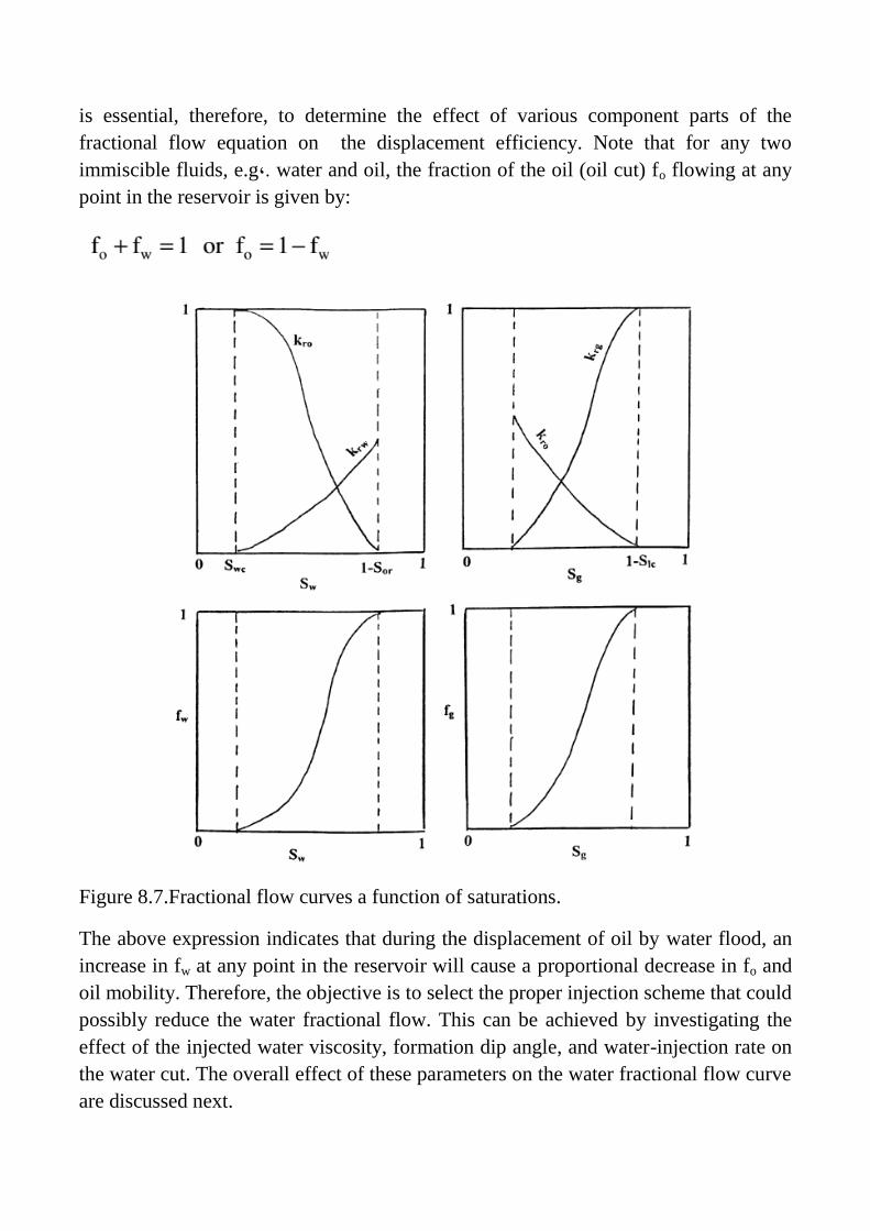
From the definition of water cut, i.e., fw=qw/(qw+ qo), we can see that the limits of

the water cut are 0% and 100%. At the irreducible (connate) water saturation, the

water flow rate qw is zero and, therefore, the water cut is 0%. At the residual oil

saturation point, Sor, the oil flow rate is zero and the water cut reaches its upper limit

of 100%. The shape of the water cut versus water saturation curve is characteristically

S-shaped, as shown in Figure 8.7. The limits of the fw curve (0 and 1) are defined by

the end points of the relative permeability curves. The implications of the above

discussion are also applied to defining the relationship that exists between fg and gas

saturation, as shown in Figure 8.7.

Note that, in general, any influences that cause the fractional flow curve to shift

upward (i.e., increase in fw or fg) will result in a less efficient displacement process. It

is essential, therefore, to determine the effect of various component parts of the

fractional flow equation on the displacement efficiency. Note that for any two

immiscible fluids, e.g,. water and oil, the fraction of the oil (oil cut) fo flowing at any

point in the reservoir is given by:

Figure 8.7.Fractional flow curves a function of saturations.

The above expression indicates that during the displacement of oil by water flood, an

increase in fw at any point in the reservoir will cause a proportional decrease in fo and

oil mobility. Therefore, the objective is to select the proper injection scheme that could

possibly reduce the water fractional flow. This can be achieved by investigating the

effect of the injected water viscosity, formation dip angle, and water-injection rate on

the water cut. The overall effect of these parameters on the water fractional flow curve

are discussed next.