CHAPTER FIVE SOLUTIONS - Innovative Learning Solutions ... · PDF fileCHAPTER FIVE SOLUTIONS Engineering Circuit Analysis, 6th Edition Copyright ©2002 McGraw-Hill, Inc. All Rights

CHAPTER FIVE SOLUTIONS

Engineering Circuit Analysis, 6th Edition Copyright ©2002 McGraw-Hill, Inc. All Rights Reserved.

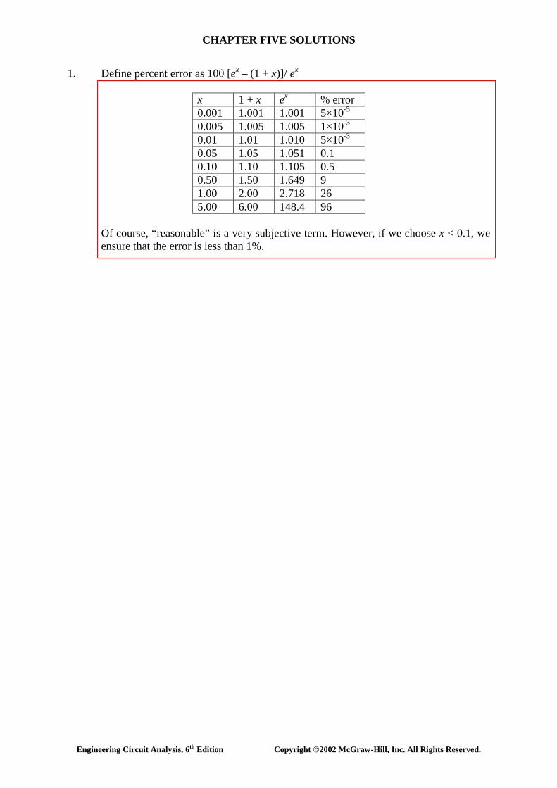
1. Define percent error as 100 [ex – (1 + x)]/ ex

x 1 + x ex % error 0.001 1.001 1.001 5×10-5 0.005 1.005 1.005 1×10-3 0.01 1.01 1.010 5×10-3 0.05 1.05 1.051 0.1 0.10 1.10 1.105 0.5 0.50 1.50 1.649 9 1.00 2.00 2.718 26 5.00 6.00 148.4 96

Of course, “reasonable” is a very subjective term. However, if we choose x < 0.1, we ensure that the error is less than 1%.



2. iA, vB “on”, vC = 0: ix = 20 A iA, vC “on”, vB = 0: ix = -5 A iA, vB, vC “on” : ix = 12 A so, we can write ix’ + ix” + ix”’ = 12 ix’ + ix” = 20 ix’ + ix”’ = - 5

In matrix form,

=

′′′′′′

5-2012

1 0 10 1 11 1 1

x

x

x

iii

(a) with iA on only, the response ix = ix’ = 3 A. (b) with vB on only, the response ix = ix” = 17 A. (c) with vC on only, the response ix = ix”’ = -8 A. (d) iA and vC doubled, vB reversed: 2(3) + 2(-8) + (-1)(17) = -27 A.



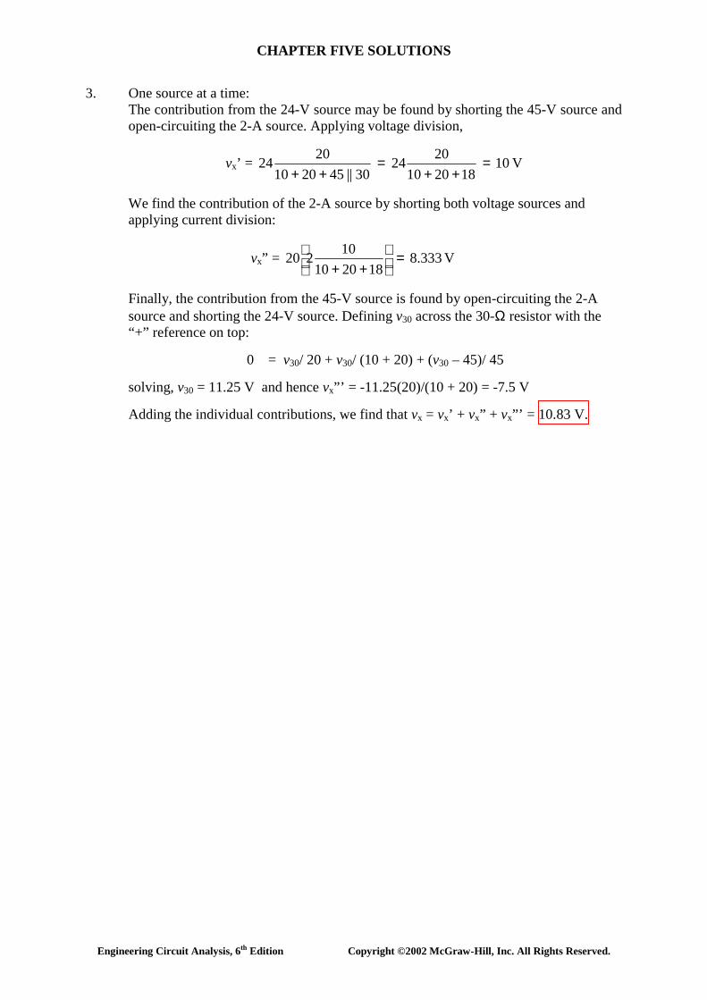
3. One source at a time: The contribution from the 24-V source may be found by shorting the 45-V source and open-circuiting the 2-A source. Applying voltage division,

vx’ = V 10 182010

2024 30||452010

2024 =++

=++

We find the contribution of the 2-A source by shorting both voltage sources and

applying current division:

vx” = V 8.333 182010

10220 =

++

Finally, the contribution from the 45-V source is found by open-circuiting the 2-A

source and shorting the 24-V source. Defining v30 across the 30-Ω resistor with the “+” reference on top:

0 = v30/ 20 + v30/ (10 + 20) + (v30 – 45)/ 45

solving, v30 = 11.25 V and hence vx”’ = -11.25(20)/(10 + 20) = -7.5 V Adding the individual contributions, we find that vx = vx’ + vx” + vx”’ = 10.83 V.



4. The contribution of the 8-A source is found by shorting out the two voltage sources and employing simple current division:

i3' = A 5- 3050

508 =+

− The contribution of the voltage sources may be found collectively or individually. The

contribution of the 100-V source is found by open-circuiting the 8-A source and shorting the 60-V source. Then,

i3" = A 6.25 30||60||)3050(

100 =+

The contribution of the 60-V source is found in a similar way as i3"' = -60/30 = -2 A. The total response is i3 = i3' + i3" + i3"' = -750 mA.



5. (a) By current division, the contribution of the 1-A source i2’ is i2’ = 1 (200)/ 250 = 800 mA. The contribution of the 100-V source is i2” = 100/ 250 = 400 mA. The contribution of the 0.5-A source is found by current division once the 1-A source is open-circuited and the voltage source is shorted. Thus,

i2”’ = 0.5 (50)/ 250 = 100 mA Thus, i2 = i2’ + i2” + i2”’ = 1.3 A

(b) P1A = (1) [(200)(1 – 1.3)] = 60 W

P200 = (1 – 1.3)2 (200) = 18 W P100V = -(1.3)(100) = -130 W P50 = (1.3 – 0.5)2 (50) = 32 W P0.5A = (0.5) [(50)(1.3 – 0.5)] = 20 W Check: 60 + 18 + 32 + 20 = +130.



6. We find the contribution of the 4-A source by shorting out the 100-V source and analysing the resulting circuit:

4 = V1' / 20 + (V1' – V')/ 10 [1] 0.4 i1' = V1'/ 30 + (V' – V1')/ 10 [2] where i1' = V1'/ 20 Simplifying & collecting terms, we obtain 30 V1' – 20 V' = 800 [1] -7.2 V1' + 8 V' = 0 [2]

Solving, we find that V' = 60 V. Proceeding to the contribution of the 60-V source, we analyse the following circuit after defining a clockwise mesh current ia flowing in the left mesh and a clockwise mesh current ib flowing in the right mesh.

30 ia – 60 + 30 ia – 30 ib = 0 [1] ib = -0.4 i1" = +0.4 ia [2]

Solving, we find that ia = 1.25 A and so V" = 30(ia – ib) = 22.5 V. Thus, V = V' + V" = 82.5 V.

'

'

"

"

'

"



7. (a) Linearity allows us to consider this by viewing each source as being scaled by 25/ 10. This means that the response (v3) will be scaled by the same factor:

25 iA'/ 10 + 25 iB'/ 10 = 25 v3'/ 10

∴ v3 = 25v3'/ 10 = 25(80)/ 10 = 200 V

(b) iA' = 10 A, iB' = 25 A → v4' = 100 V iA" = 10 A, iB" = 25 A → v4" = -50 V iA = 20 A, iB = -10 A → v4 = ? We can view this in a somewhat abstract form: the currents iA and iB multiply the same circuit parameters regardless of their value; the result is v4.

Writing in matrix form,

=

50-

100

ba

10 2525 10

, we can solve to find

a = -4.286 and b = 5.714, so that 20a – 10b leads to v4 = -142.9 V



8. With the current source open-circuited and the 7-V source shorted, we are left with 100k || (22k + 4.7k) = 21.07 kΩ.

Thus, V3V = 3 (21.07)/ (21.07 + 47) = 0.9286 V. In a similar fashion, we find that the contribution of the 7-V source is: V7V = 7 (31.97) / (31.97 + 26.7) = 3.814 V Finally, the contribution of the current source to the voltage V across it is: V5mA = (5×10-3) ( 47k || 100k || 26.7k) = 72.75 V. Adding, we find that V = 0.9286 + 3.814 + 72.75 = 77.49 V.



9. We must find the current through the 500-kΩ resistor using superposition, and then calculate the dissipated power.

The contribution from the current source may be calculated by first noting that

1M || 2.7M || 5M = 636.8 kΩ. Then,

i60µA = A 43.51 0.636830.5

3 1060 6 µ=

++× −

The contribution from the voltage source is found by first noting that 2.7M || 5M =

1.753 MΩ. The total current flowing from the voltage source (with the current source open-circuited) is –1.5/ (3.5 || 1.753 + 1) µA = -0.6919 µA. The current flowing through the 500-kΩ resistor due to the voltage source acting alone is then

i1.5V = 0.6919 (1.753)/ (1.753 + 3.5) mA = 230.9 nA.

The total current through the 500-kΩ resistor is then i60µA + i1.5V = 43.74 µA and the

dissipated power is (43.74×10-9)2 (500×103) = 956.6 µW.



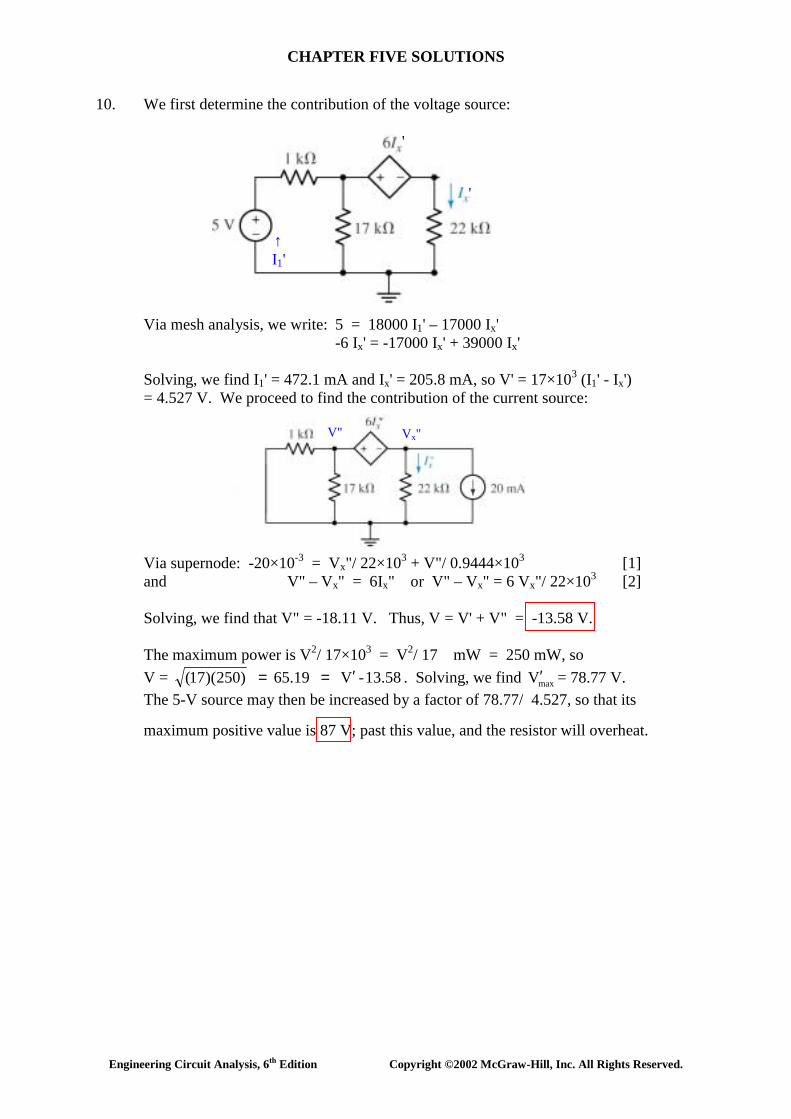
10. We first determine the contribution of the voltage source:

Via mesh analysis, we write: 5 = 18000 I1' – 17000 Ix' -6 Ix' = -17000 Ix' + 39000 Ix' Solving, we find I1' = 472.1 mA and Ix' = 205.8 mA, so V' = 17×103 (I1' - Ix')

= 4.527 V. We proceed to find the contribution of the current source: Via supernode: -20×10-3 = Vx"/ 22×103 + V"/ 0.9444×103 [1] and V" – Vx" = 6Ix" or V" – Vx" = 6 Vx"/ 22×103 [2] Solving, we find that V" = -18.11 V. Thus, V = V' + V" = -13.58 V.

The maximum power is V2/ 17×103 = V2/ 17 mW = 250 mW, so V = 13.58 - V 65.19 )250)(17( ′== . Solving, we find maxV′ = 78.77 V. The 5-V source may then be increased by a factor of 78.77/ 4.527, so that its maximum positive value is 87 V; past this value, and the resistor will overheat.

'

↑ I1'

'

Vx" V"



11. It is impossible to identify the individual contribution of each source to the power dissipated in the resistor; superposition cannot be used for such a purpose.

Simplifying the circuit, we may at least determine the total power dissipated in the

resistor: Via superposition in one step, we may write

i = mA 195.1 2.12

2.12 - 1.22

5 =++

Thus, P2Ω = i2 . 2 = 76.15 mW

i →



12. We will analyse this circuit by first considering the combined effect of both dc sources (left), and then finding the effect of the single ac source acting alone (right).

1, 3 supernode: V1/ 100 + V1/ 17×103 + (V1 – 15)/ 33×103 + V3/ 103 = 20 IB [1] and: V1 – V3 = 0.7 [2] Node 2: -20 IB = (V2 – 15)/ 1000 [3] We require one additional equation if we wish to have IB as an unknown: 20 IB + IB = V3/ 1000 [4] Simplifying and collecting terms,

10.08912 V1 + V3 – 20×103 IB = 0.4545 [1] V1 - V3 = 0.7 [2]

V2 + 20×103 IB = 15 [3]

-V3 + 21×103 IB = 0 [4]

Solving, we find that IB = -31.04 µA. To analyse the right-hand circuit, we first find the Thévenin equivalent to the left of

the wire marked iB', noting that the 33-kΩ and 17-kΩ resistors are now in parallel. We find that VTH = 16.85 cos 6t V by voltage division, and RTH = 100 || 17k || 33k = 99.12 Ω. We may now proceed:

20 iB' = vx' / 1000 + (vx' – 16.85 cos 6t)/ 99.12 [1] 20 iB' + iB'' = vx'/ 1000 [2]

Solving, we find that iB' = 798.6 cos 6t mA. Thus, adding our two results, we find the complete current is

iB = iB' + IB = -31.04 + 798.6 cos 6t µA.

IB

IB

V1

V2

V3 vx'



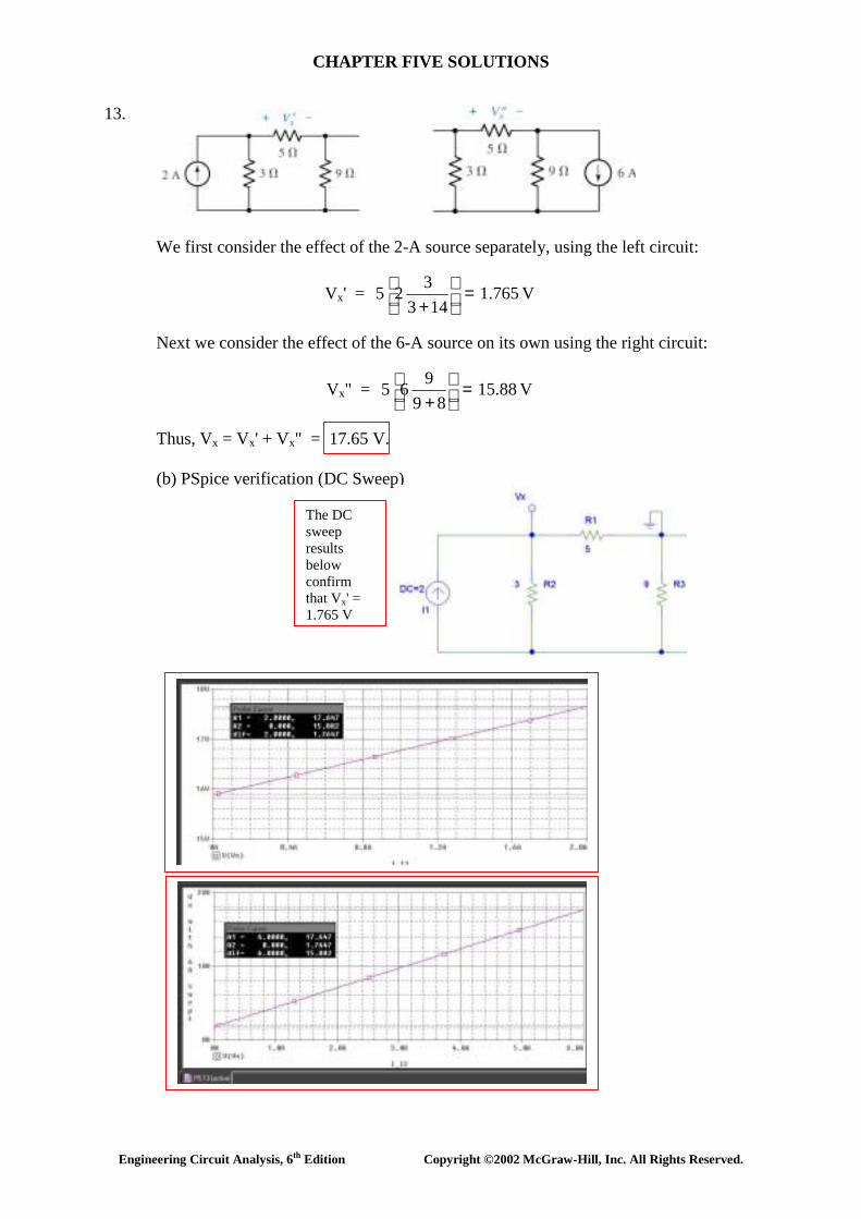
13. We first consider the effect of the 2-A source separately, using the left circuit:

Vx' = V 1.765 143

3 2 5 =

+

Next we consider the effect of the 6-A source on its own using the right circuit:

Vx" = V 15.88 89

9 6 5 =

+

Thus, Vx = Vx' + Vx" = 17.65 V. (b) PSpice verification (DC Sweep)

The DC sweep results below confirm that Vx' = 1.765 V



14. (a) Beginning with the circuit on the left, we find the contribution of the 2-V source to

Vx:

502V

100V V4 xx

x−′

+′

=′−

which leads to Vx' = 9.926 mV. The circuit on the right yields the contribution of the 6-A source to Vx:

50V

100V V4 xx

x′′

+′′

=′′−

which leads to Vx" = 0. Thus, Vx = Vx' + Vx" = 9.926 mV. (b) PSpice verification.

'

As can be seen from the two separate PSpice simulations, our hand calculations are correct; the pV-scale voltage in the second simulation is a result of numerical inaccuracy.



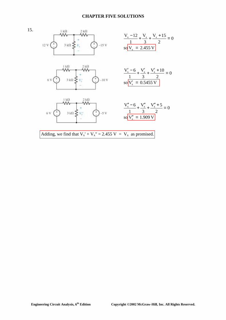
15.

V 2.455 V so

02

15V3

V1

12V

x

xxx

=

=+++−

V 0.5455 V so

02

10V3

V1

6V

x

xxx

=′

=+′+

′+−′

V 1.909 V so

02

5V3

V1

6V

x

xxx

=′′

=+′′+

′′+−′′

Adding, we find that Vx' + Vx" = 2.455 V = Vx as promised.



16. (a) [120 cos 400t] / 60 = 2 cos 400t A. 60 || 120 = 40 Ω.

[2 cos 400t] (40) = 80 cos 400t V. 40 + 10 = 50 Ω.

[80 cos 400t]/ 50 = 1.6 cos 400t A. 50 || 50 = 25 Ω. (b) 2k || 3k + 6k = 7.2 kΩ. 7.2k || 12k = 4.5 kΩ (20)(4.5) = 90 V.

25 Ω 1.6 cos 400t A

4.5 kΩ

3.5 kΩ

8 kΩ



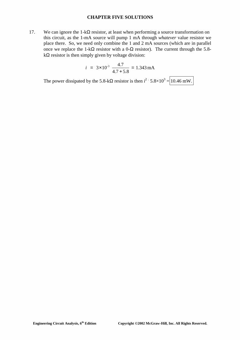
17. We can ignore the 1-kΩ resistor, at least when performing a source transformation on this circuit, as the 1-mA source will pump 1 mA through whatever value resistor we place there. So, we need only combine the 1 and 2 mA sources (which are in parallel once we replace the 1-kΩ resistor with a 0-Ω resistor). The current through the 5.8-kΩ resistor is then simply given by voltage division:

mA 1.343 5.84.7

4.7 103 3- =+

×=i

The power dissipated by the 5.8-kΩ resistor is then i2 . 5.8×103 = 10.46 mW.



18. We may ignore the 10-kΩ and 9.7-kΩ resistors, as 3-V will appear across them regardless of their value. Performing a quick source transformation on the 10-kΩ resistor/ 4-mA current source combination, we replace them with a 40-V source in series with a 10-kΩ resistor:

I = 43/ 15.8 mA = 2.722 mA. Therefore, P5.8Ω = I2. 5.8×103 = 42.97 mW.

Ω

Ω

I →



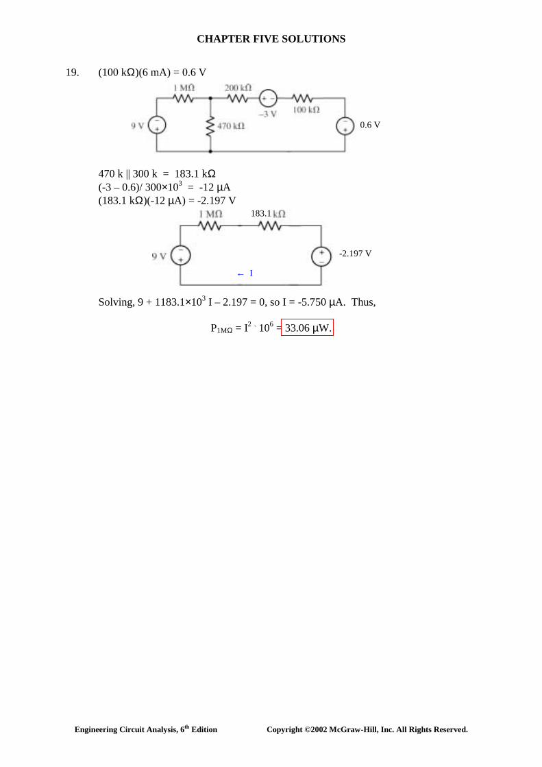
19. (100 kΩ)(6 mA) = 0.6 V

470 k || 300 k = 183.1 kΩ (-3 – 0.6)/ 300×103 = -12 µA (183.1 kΩ)(-12 µA) = -2.197 V Solving, 9 + 1183.1×103 I – 2.197 = 0, so I = -5.750 µA. Thus,

P1MΩ = I2 . 106 = 33.06 µW.

0.6 V

183.1

-2.197 V

← I



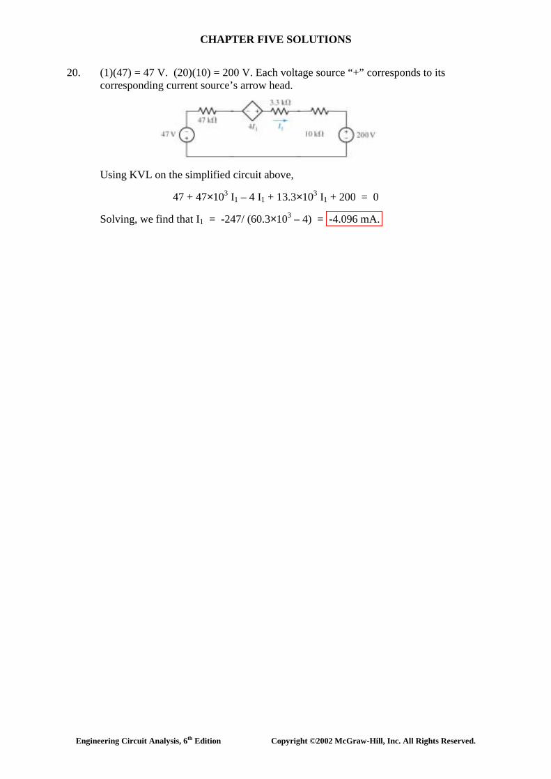
20. (1)(47) = 47 V. (20)(10) = 200 V. Each voltage source “+” corresponds to its corresponding current source’s arrow head.

Using KVL on the simplified circuit above,

47 + 47×103 I1 – 4 I1 + 13.3×103 I1 + 200 = 0

Solving, we find that I1 = -247/ (60.3×103 – 4) = -4.096 mA.



21. (2 V1)(17) = 34 V1

Analysing the simplified circuit above,

34 V1 – 0.6 + 7 I + 2 I + 17 I = 0 [1] and V1 = 2 I [2]

Substituting, we find that I = 0.6/ (68 + 7 + 2 + 17) = 6.383 mA. Thus,

V1 = 2 I = 12.77 mV

34

← I



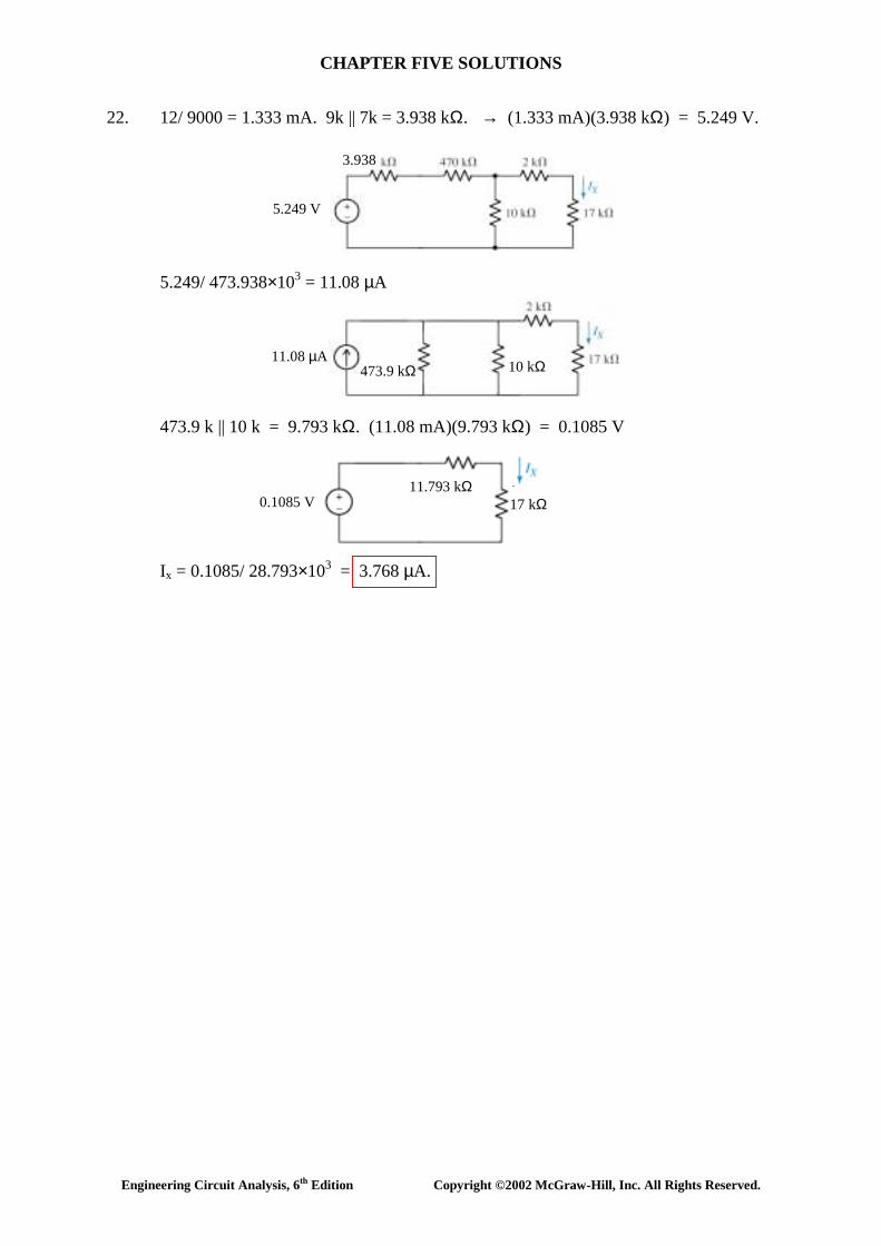
22. 12/ 9000 = 1.333 mA. 9k || 7k = 3.938 kΩ. → (1.333 mA)(3.938 kΩ) = 5.249 V. 5.249/ 473.938×103 = 11.08 µA 473.9 k || 10 k = 9.793 kΩ. (11.08 mA)(9.793 kΩ) = 0.1085 V Ix = 0.1085/ 28.793×103 = 3.768 µA.

5.249 V

3.938

473.9 kΩ 10 kΩ

11.08 µA

0.1085 V 17 kΩ

11.793 kΩ



23. First, (-7 µA)(2 MΩ) = -14 V, “+” reference down. 2 MΩ + 4 MΩ = 6 MΩ. +14 V/ 6 ΜΩ = 2.333 µA, arrow pointing up; 6 M || 10 M = 3.75 MΩ.

(2.333)(3.75) = 8.749 V. Req = 6.75 MΩ ∴ Ix = 8.749/ (6.75 + 4.7) µA = 764.1 nA.

2.333

3.75 MΩ



24. To begin, note that (1 mA)(9 Ω) = 9 mV, and 5 || 4 = 2.222 Ω. The above circuit may not be further simplified using only source transformation

techniques.

9

15

2.222 Ω



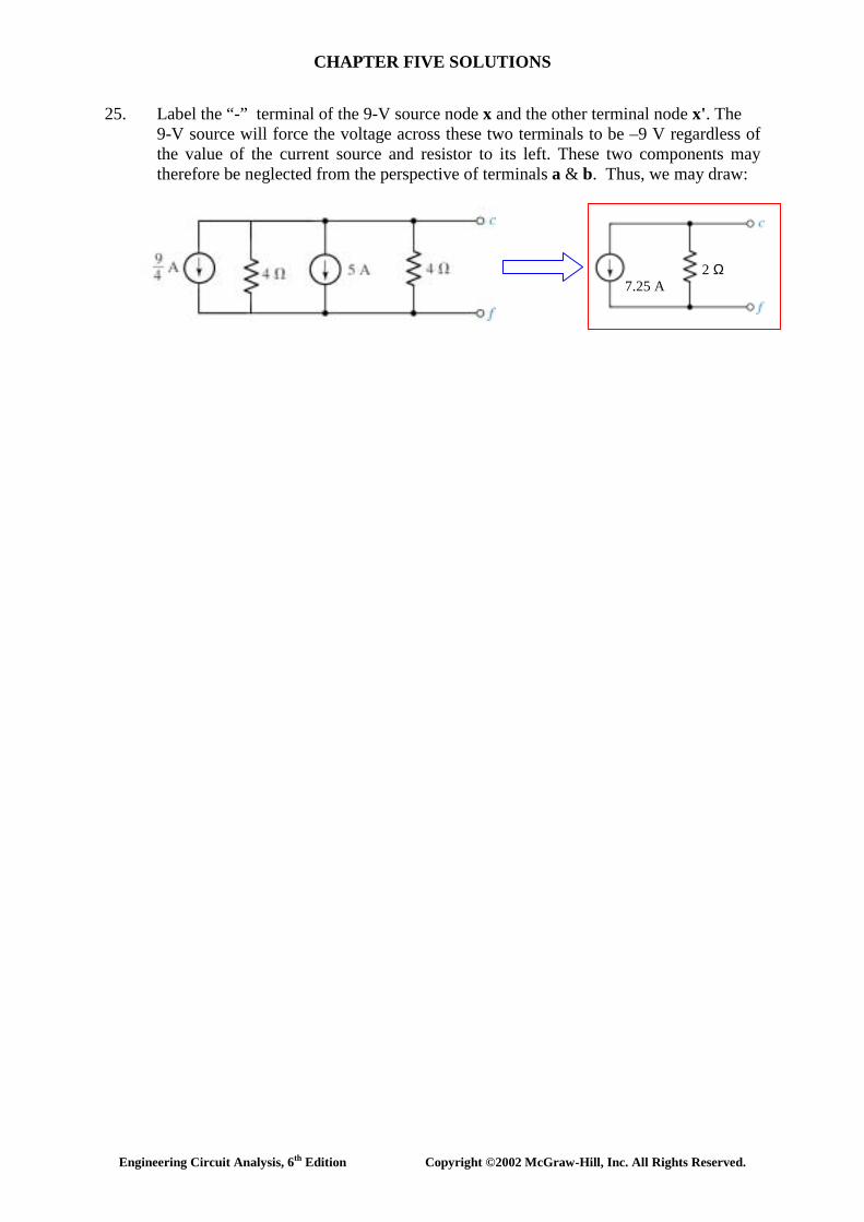
25. Label the “-” terminal of the 9-V source node x and the other terminal node x'. The 9-V source will force the voltage across these two terminals to be –9 V regardless of the value of the current source and resistor to its left. These two components may therefore be neglected from the perspective of terminals a & b. Thus, we may draw:

7.25 A 2 Ω



26. Beware of the temptation to employ superposition to compute the dissipated power- it won’t work!

Instead, define a current I flowing into the bottom terminal of the 1-MΩ resistor.

Using superposition to compute this current,

I = 1.8/ 1.840 + 0 + 0 µA = 978.3 nA. Thus,

P1MΩ = (978.3×10-9)2 (106) = 957.1 nW.



27. Let’s begin by plotting the experimental results, along with a least-squares fit to part of the data:

We see from the figure that we cannot draw a very good line through all data points

representing currents from 1 mA to 20 mA. We have therefore chosen to perform a linear fit for the three lower voltages only, as shown. Our model will not be as accurate at 1 mA; there is no way to know if our model will be accurate at 20 mA, since that is beyond the range of the experimental data. Modeling this system as an ideal voltage source in series with a resistance (representing the internal resistance of the battery) and a varying load resistance, we may write the following two equations based on the linear fit to the data:

1.567 = Vsrc – Rs (1.6681×10-3) 1.558 = Vsrc – Rs (12.763×10-3)

Solving, Vsrc = 1.568 V and Rs = 811.2 mΩ. It should be noted that depending on the line fit to the experimental data, these values can change somewhat, particularly the series resistance value.

Least-squares fit results: Voltage (V) Current (mA) 1.567 1.6681 1.563 6.599 1.558 12.763



28. Let’s begin by plotting the experimental results, along with a least-squares fit to part of the data:

We see from the figure that we cannot draw a very good line through all data points

representing currents from 1 mA to 20 mA. We have therefore chosen to perform a linear fit for the three lower voltages only, as shown. Our model will not be as accurate at 1 mA; there is no way to know if our model will be accurate at 20 mA, since that is beyond the range of the experimental data. Modeling this system as an ideal current source in parallel with a resistance Rp (representing the internal resistance of the battery) and a varying load resistance, we may write the following two equations based on the linear fit to the data: 1.6681×10-3 = Isrc – 1.567/ Rp 12.763×10-3 = Isrc – 1.558/ Rp

Solving, Isrc = 1.933 A and Rs = 811.2 mΩ. It should be noted that depending on the line fit to the experimental data, these values can change somewhat, particularly the series resistance value.

Least-squares fit results: Voltage (V) Current (mA) 1.567 1.6681 1.563 6.599 1.558 12.763



29. Reference terminals are required to avoid ambiguity: depending on the sources with which we begin the transformation process, we will obtain entirely different answers. Working from left to right in this case,

2 µA – 1.8 µA = 200 nA, arrow up. 1.4 MΩ + 2.7 MΩ = 4.1 MΩ

An additional transformation back to a voltage source yields (200 nA)(4.1 MΩ) = 0.82 V in series with 4.1 MΩ + 2 MΩ = 6.1 MΩ, as shown below:

Then, 0.82 V/ 6.1 MΩ = 134.4 nA, arrow up. 6.1 MΩ || 3 MΩ = 2.011 MΩ 4.1 µA + 134.4 nA = 4.234 mA, arrow up. (4.234 µA) (2.011 MΩ) = 8.515 V.

±

6.1

0.82 V

± 8.515 V

2.011



30. To begin, we note that the 5-V and 2-V sources are in series: Next, noting that 3 V/ 1 Ω = 3 A, and 4 A – 3 A = +1 A (arrow down), we obtain: By voltage division, the voltage across the 5-Ω resistor in the circuit to the right is:

(-1) 2 5||2

5||2+

= -0.4167 V.

Thus, the power dissipated by the 5-Ω resistor is (-0.4167)2 / 5 = 34.73 mW.

3

The left-hand resistor and the current source are easily transformed into a 1-V source in series with a 1-Ω resistor:

± -1 V



31. (a) RTH = 25 || (10 + 15) = 25 || 25 = 12.5 Ω.

VTH = Vab =

++++

++ 2510151015 100

25151025 50 = 75 V.

(b) If Rab = 50 Ω,

P50Ω = W72 501

12.55050 75

2

=

+

(c) If Rab = 12.5 Ω,

P12.5Ω = W112.5 12.5

1 12.55.21

12.5 752

=

+



32. (a) Removing terminal c, we need write only one nodal equation:

0.1 = 15

5V 12

2V bb −+− , which may be solved to

yield Vb = 4 V. Therefore, Vab = VTH = 2 – 4 = -2 V. RTH = 12 || 15 = 6.667 Ω. We may then calculate IN as IN = VTH/ RTH = -300 mA (arrow pointing upwards).

(b) Removing terminal a, we again find RTH = 6.667 Ω, and only need write a single nodal equation; in fact, it is identical to that written for the circuit above, and we once again find that Vb = 4 V. In this case, VTH = Vbc = 4 – 5 = -1 V, so IN = -1/ 6.667 = -150 mA (arrow pointing upwards).



33. (a) Shorting out the 88-V source and open-circuiting the 1-A source, we see looking into the terminals x and x' a 50-Ω resistor in parallel with 10 Ω in parallel with

(20 Ω + 40 Ω), so RTH = 50 || 10 || (20 + 40) = 7.317 Ω

Using superposition to determine the voltage Vxx' across the 50-Ω resistor, we find

Vxx' = VTH =

++

+

++

+)10||50(2040

4010)||(1)(50 )]4020(||50[10

)4020(||5088

=

+++

333.8204040(1)(8.333)

27.3727.2788 = 69.27 V

(b) Shorting out the 88-V source and open-circuiting the 1-A source, we see looking

into the terminals y and y' a 40-Ω resistor in parallel with [20 Ω + (10 Ω || 50 Ω)]:

RTH = 40 || [20 + (10 || 50)] = 16.59 Ω Using superposition to determine the voltage Vyy' across the 1-A source, we find

Vyy' = VTH = (1)(RTH) +

+

+ 402040

27.271027.2788

= 59.52 V



34. (a) Select terminal b as the reference terminal, and define a nodal voltage V1 at the top of the 200-Ω resistor. Then,

0 = 200V

100VV

4020V 1TH11 +−+− [1]

1.5 i1 = (VTH – V1)/ 100 [2]

where i1 = V1/ 200, so Eq. [2] becomes 150 V1/ 200 + V1 - VTH = 0 [2] Simplifying and collecting terms, these equations may be re-written as:

(0.25 + 0.1 + 0.05) V1 – 0.1 VTH = 5 [1] (1 + 15/ 20) V1 – VTH = 0 [2]

Solving, we find that VTH = 38.89 V. To find RTH, we short the voltage source and

inject 1 A into the port:

0 = 200V

40V

100VV 11in1 ++− [1]

1.5 i1 + 1 = 100

VV 1in − [2]

i1 = V1/ 200 [3] Combining Eqs. [2] and [3] yields 1.75 V1 – Vin = -100 [4] Solving Eqs. [1] & [4] then results in Vin = 177.8 V, so that RTH = Vin/ 1 A = 177.8 Ω.

(b) Adding a 100-Ω load to the original circuit or our Thévenin equivalent, the

voltage across the load is

V100Ω = V 14.00 177.8100

100 VTH =

+, and so P100Ω = (V100Ω)2 / 100 = 1.96 W.

1 A

+

Vin -

V1

Ref.



35. We inject a current of 1 A into the port (arrow pointing up), select the bottom terminal as our reference terminal, and define the nodal voltage Vx across the 200-Ω resistor.

Then, 1 = V1/ 100 + (V1 – Vx)/ 50 [1] -0.1 V1 = Vx/ 200 + (Vx – V1)/ 50 [2] which may be simplified to

3 V1 – 2 Vx = 100 [1] 16 V1 + 5 Vx = 0 [2]

Solving, we find that V1 = 10.64 V, so RTH = V1/ (1 A) = 10.64 Ω.

Since there are no independent sources present in the original network, IN = 0.



36. With no independent sources present, VTH = 0. We decide to inject a 1-A current into the port: Node ‘x’: 0.01 vab = vx/ 200 + (vx – vf)/ 50 [1] Supernode: 1 = vab/ 100 + (vf – vx) [2] and: vab – vf = 0.2 vab [3] Rearranging and collecting terms, -2 vab + 5 vx – 4 vf = 0 [1] vab – 2 vx + 2 vf = 100 [2] 0.8 vab - vf = 0 [3]

Solving, we find that vab = 192.3 V, so RTH = vab/ (1 A) = 192.3 Ω.

Ref.

vx

vf •

A



37. We first find RTH by shorting out the voltage source and open-circuiting the current source.

Looking into the terminals a & b, we see RTH = 10 || [47 + (100 || 12)]

= 8.523 Ω. Returning to the original circuit, we decide to perform nodal analysis to obtain VTH:

-12×103 = (V1 – 12)/ 100×103 + V1/ 12×103 + (V1 – VTH)/ 47×103 [1]

12×103 = VTH/ 10×103 + (VTH – V1)/ 47×103 [2]

Rearranging and collecting terms,

0.1146 V1 - 0.02128 VTH = -11.88 [1] -0.02128 V1 + 0.02128 VTH = 12 [2]

Solving, we find that VTH = 83.48 V.



38. (a) RTH = 4 + 2 || 2 + 10 = 15 Ω. (b) same as above: 15 Ω.



39. For Fig. 5.78a, IN = 12/ ~0 → ∞ A in parallel with ~ 0 Ω. For Fig. 5.78b, VTH = (2)(~∞) → ∞ V in series with ~∞ Ω.



40. With no independent sources present, VTH = 0. Connecting a 1-V source to the port and measuring the current that flows as a result, I = 0.5 Vx + 0.25 Vx = 0.5 + 0.25 = 0.75 A.

RTH = 1/ I = 1.333 Ω.

The Norton equivalent is 0 A in parallel with 1.333 Ω.

+ -

← I



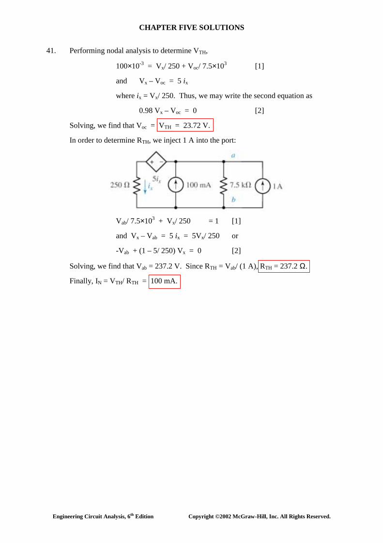
41. Performing nodal analysis to determine VTH,

100×10-3 = Vx/ 250 + Voc/ 7.5×103 [1] and Vx – Voc = 5 ix where ix = Vx/ 250. Thus, we may write the second equation as 0.98 Vx – Voc = 0 [2] Solving, we find that Voc = VTH = 23.72 V. In order to determine RTH, we inject 1 A into the port:

Vab/ 7.5×103 + Vx/ 250 = 1 [1] and Vx – Vab = 5 ix = 5Vx/ 250 or -Vab + (1 – 5/ 250) Vx = 0 [2]

Solving, we find that Vab = 237.2 V. Since RTH = Vab/ (1 A), RTH = 237.2 Ω. Finally, IN = VTH/ RTH = 100 mA.



42. We first note that VTH = Vx, so performing nodal analysis, -5 Vx = Vx/ 19 which has the solution Vx = 0 V.

Thus, VTH (and hence IN) = 0. (Assuming RTH ≠ 0) To find RTH, we inject 1 A into the port, noting that RTH = Vx/ 1 A:

-5 Vx + 1 = Vx/ 19 Solving, we find that Vx = 197.9 mV, so that RTH = RN = 197.9 mV.



43. Shorting out the voltage source, we redraw the circuit with a 1-A source in place of the 2-kΩ resistor:

Noting that 300 Ω || 2 MΩ ≈ 300 Ω, 0 = (vgs – V)/ 300 [1] 1 – 0.02 vgs = V/ 1000 + (V – vgs)/ 300 [2] Simplifying & collecting terms, vgs – V = 0 [1] 0.01667 vgs + 0.00433 V = 1 [2]

Solving, we find that vgs = V = 47.62 V. Hence, RTH = V/ 1 A = 47.62 Ω.

1 A

Ref.

V



44. We replace the source vs and the 300-Ω resistor with a 1-A source and seek its voltage:

By nodal analysis, 1 = V1/ 2×106 so V1 = 2×106 V.

Since V = V1, we have Rin = V/ 1 A = 2 MΩ.

1 A

+

V -

Ref.

V1 V2



45. Removing the voltage source and the 300-Ω resistor, we replace them with a 1-A source and seek the voltage that develops across its terminals:

We select the bottom node as our reference terminal, and define nodal voltages V1

and V2. Then,

1 = V1 / 2×106 + (V1 – V2)/ rπ [1]

0.02 vπ = (V2 – V1)/ rπ + V2/ 1000 + V2/ 2000 [2]

where vπ = V1 – V2 Simplifying & collecting terms,

(2×106 + rπ) V1 – 2×106 V2 = 2×106 rπ [1]

-(2000 + 40 rπ) V1 + (2000 + 43 rπ) V2 = 0 [2]

Solving, we find that V1 = V =

++×

+×π

π

r 14.33 666.7 102r 14.33 666.7 102 6

6 .

Thus, RTH = 2×106 || (666.7 + 14.33 rπ) Ω.

1 A

+

V -

Ref.



46. Such a scheme probably would lead to maximum or at least near-maximum power transfer to our home. Since we pay the utility company based on the power we use, however, this might not be such a hot idea…



47. We need to find the Thévenin equivalent resistance of the circuit connected to RL, so we short the 20-V source and open-circuit the 2-A source; by inspection, then

RTH = 12 || 8 + 5 + 6 = 15.8 Ω Analyzing the original circuit to obtain V1 and V2 with RL removed: V1 = 20 8/ 20 = 8 V; V2 = -2 (6) = -12 V. We define VTH = V1 – V2 = 8 + 12 = 20 V. Then,

PRL|max = W6.329 4(15.8)

400 R 4

V

L

2TH ==

+ VTH -

V1 V2

Ref.



48. (a) RTH = 25 || (10 + 15) = 12.5 Ω

Using superposition, Vab = VTH = 50

1015100 251015

2550 ++++

= 75 V.

(b) Connecting a 50-Ω resistor,

Pload = W90 50 12.5

75 R R

V 2

loadTH

2TH =

+=

+

(c) Connecting a 12.5-Ω resistor,

Pload = ( ) W112.5 12.5 475

R 4V 2

TH

2TH ==



49. (a) By inspection, we see that i10 = 5 A, so VTH = Vab = 2(0) + 3 i10 + 10 i10 = 13 i10 = 13(5) = 65 V.

To find RTH, we connect a 1-A source between terminals a & b: 5 = V1/ 10 + (V2 – V)/ 2 [1] → V1 + 5 V2 – 5 V = 50 [1] 1 = (V – V2)/ 2 [2] → -V2 + V = 2 [2] and V2 – V1 = 3 i10 [3] where i10 = V1/ 10 → -13 V1 + 10 V2 = 0 [3] Solving, we find that V = 80 V, so that RTH = V / 1 A = 80 Ω.

(b) Pmax = W13.20 4(80)65

R 4V 2

TH

2TH ==

Ref.

V1 V2 V •



50. (a) Replacing the resistor RL with a 1-A source, we seek the voltage that develops across

its terminals with the independent voltage source shorted:

1 1 1

1 1

1

1

10 20 40 0 [1] 30 20 0 [1]and 1 [2] 1 [2]Solving, 400 mA

So 40 16 V and 161A

− + + = ⇒ + =− = ⇒ − =

=

= = = = Ω

x x

x x

TH

i i i i ii i i i

iVV i R

(b) Removing the resistor RL from the original circuit, we seek the resulting open-circuit

voltage:

1

1

10 500 [1]20 40

50where 40

1 50 50so [1] becomes 020 2 40 40

50020 80

0 4 505 50

or 10 V

− −= +

−=

− − = − + −= +

= + −=

=

TH TH

TH

TH TH TH

TH TH

TH TH

TH

TH

V i V

Vi

V V V

V V

V VV

V

Thus, if

16 ,

5V2

= = Ω

= = =+L

L TH

L THR TH

L TH

R RR VV V

R R

+

VTH -



51. (a) 2.5A=NI

220 802 A

==i

i

By current division,

2 2.520

=+N

N

RR

Solving, 80= = ΩN THR R Thus, 2.5 80 200V= = × =TH OCV V

(b) 2 2

max200 125 W

4 4 80= = =

×TH

TH

VPR

(c) 80= = ΩL THR R

RN 20 Ω

↓ 2 A



52.

By Voltage ÷, =+

NR N

N

RI IR R

So Solving, 1.7 A=NI and 33.33= ΩNR (a) If (b) If (c) If

is a maximum,33.33

33.331.7 850 mA33.33 33.33

33.33 28.33V

= = Ω

= × =+

= =

L L

L N

L

L L

v iR R

i

v i

is a maximum

; max when 0

So 1.7A0V

= = Ω+

==

L

NL N L

N L

L

L

iRi i R

R Ri

v

0.2 [1]250

0.5 [2]80

=+

=+

NN

N

NN

N

RIR

RIR

10 W to 250 corresp to 200mA.20 W to 80 corresp to 500mA.

ΩΩ

RN R

IN

is a maximum( )

So is a maximum when is a maximum, which occurs at . Then 0 and 1.7 56.66 V

=

= ∞= = × =

L

L N N L

L N L L

L L N

vV I R R

v R R Ri v R



53. There is no conflict with our derivation concerning maximum power. While a dead short across the battery terminals will indeed result in maximum current draw from the battery, and power is indeed proportional to i2, the power delivered to the load is i2RLOAD = i2(0) = 0 watts. This is the minimum, not the maximum, power that the battery can deliver to a load.



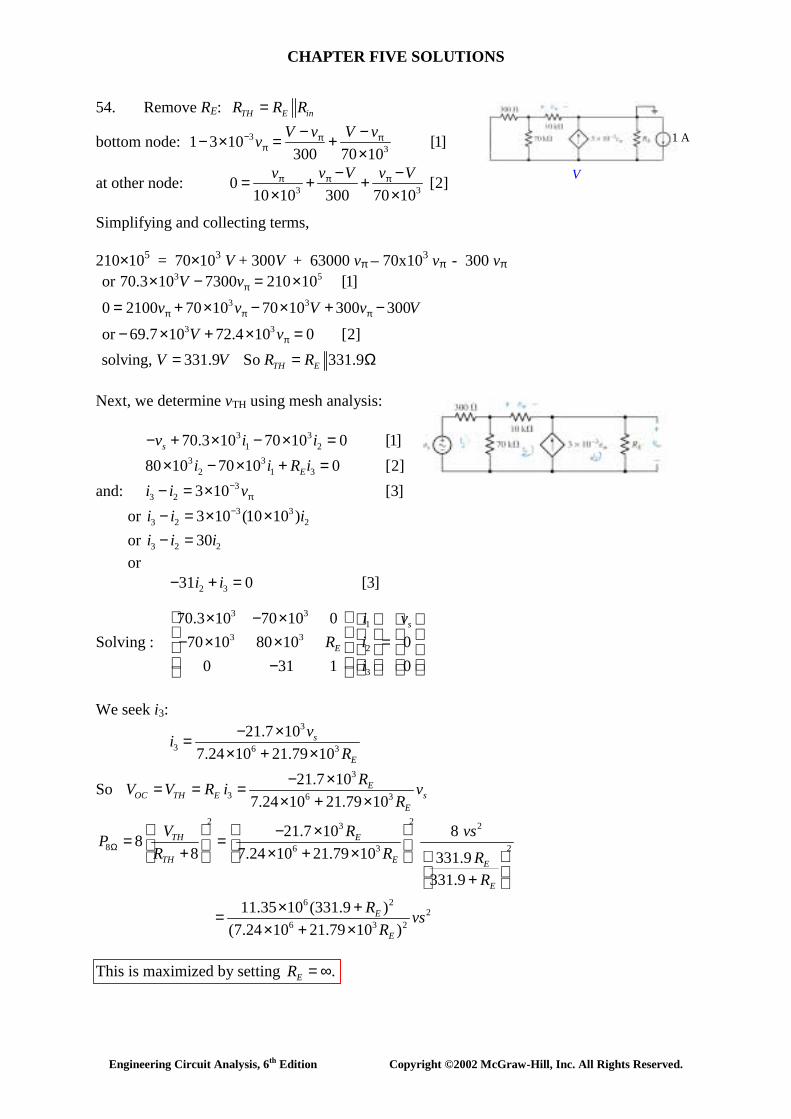
54. Remove RE: =TH E inR R R

bottom node: 331 3 10 [1]

300 70 10− π π

π− −− × = +

×V v V vv

at other node: 3 3010 10 300 70 10

π π π− −= + +× ×v v V v V [2]

Simplifying and collecting terms, 210×105 = 70×103 V + 300V + 63000 vπ – 70x103 vπ - 300 vπ

3 5

3 3

3 3

or 70.3 10 7300 210 10 [1]

0 2100 70 10 70 10 300 300

or 69.7 10 72.4 10 0 [2]solving, 331.9 So 331.9

π

π π π

π

× − = ×

= + × − × + −

− × + × == = ΩTH E

V vv v V v V

V vV V R R

Next, we determine vTH using mesh analysis: 3 3

1 270.3 10 70 10 0 [1]− + × − × =sv i i 3 3

2 1 380 10 70 10 0 [2]× − × + =Ei i R i and: 3

3 2 3 10 [3]−π− = ×i i v

or 3 33 2 23 10 (10 10 )−− = × ×i i i

or 3 2 230− =i i i or 2 331 0 [3]− + =i i

Solving :

3 31

3 32

3

70.3 10 70 10 070 10 80 10 0

0 31 1 0

× − × − × × = −

s

E

i vR i

i

We seek i3:

3

3 6 3

21.7 107.24 10 21.79 10

− ×=× + ×

s

E

viR

So 3

3 6 3

21.7 107.24 10 21.79 10

− ×= = =× + ×

EOC TH E s

E

RV V R i vR

2 23 2

8 26 3

6 22

6 3 2

21.7 10 888 7.24 10 21.79 10 331.9

331.9

11.35 10 (331.9 )(7.24 10 21.79 10 )

Ω − ×= = + × + ×

+ × +=

× + ×

TH E

TH E E

E

E

E

V R vsPR R R

R

R vsR

This is maximized by setting .= ∞ER

V

1 A



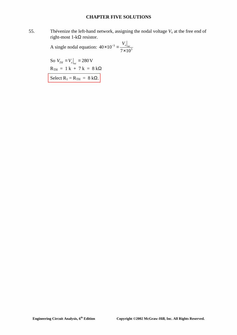
55. Thévenize the left-hand network, assigning the nodal voltage Vx at the free end of right-most 1-kΩ resistor.

A single nodal equation: 3340 10

7 10−× =

×x oc

V

So 280V= =TH x ocV V

RTH = 1 k + 7 k = 8 kΩ

Select R1 = RTH = 8 kΩ.



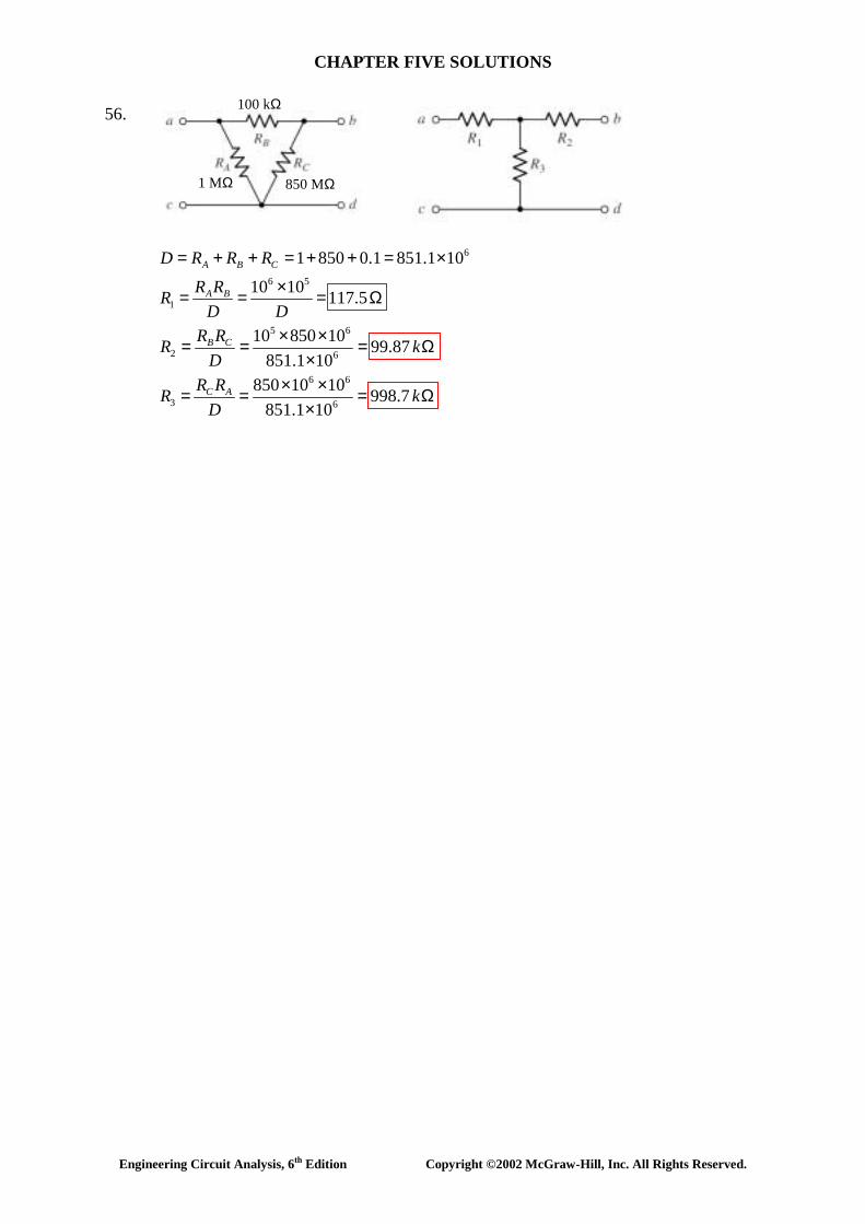
56.

6

6 5

1

5 6

2 6

6 6

3 6

1 850 0.1 851.1 10

10 10 117.5

10 850 10 99.87851.1 10

850 10 10 998.7851.1 10

= + + = + + = ×

×= = = Ω

× ×= = = Ω×

× ×= = = Ω×

A B C

A B

B C

C A

D R R RR RR

D DR RR k

DR RR k

D

1 MΩ

100 kΩ

850 MΩ



57.

1 2 2 3 3 1

2

3

1

0.1 0.4 0.4 0.9 0.9 0.10.49

1.225

544.4m

4.9

= + += × + × + ×= Ω

= = Ω

= = Ω

= = Ω

A

B

C

N R R R R R R

NRRNRRNRR

R1 R2

R3



58.

1

2

: 1 6 3 106 1 6 3 3 10.6, 1.8 , 0.310 10 10

: 5 1 4 105 1 1 4 5 40.5 , 0.4 , 210 10 10

1.8 2 0.5 4.30.3 0.6 0.4 1.31.3 4.3 0.99820.9982 0.6 2 3.5983.598 6 2.249

∆ + + = Ω× × ×= = =

∆ + + = Ω× × ×= = =

+ + = Ω+ + = Ω

= Ω+ + = Ω= Ω



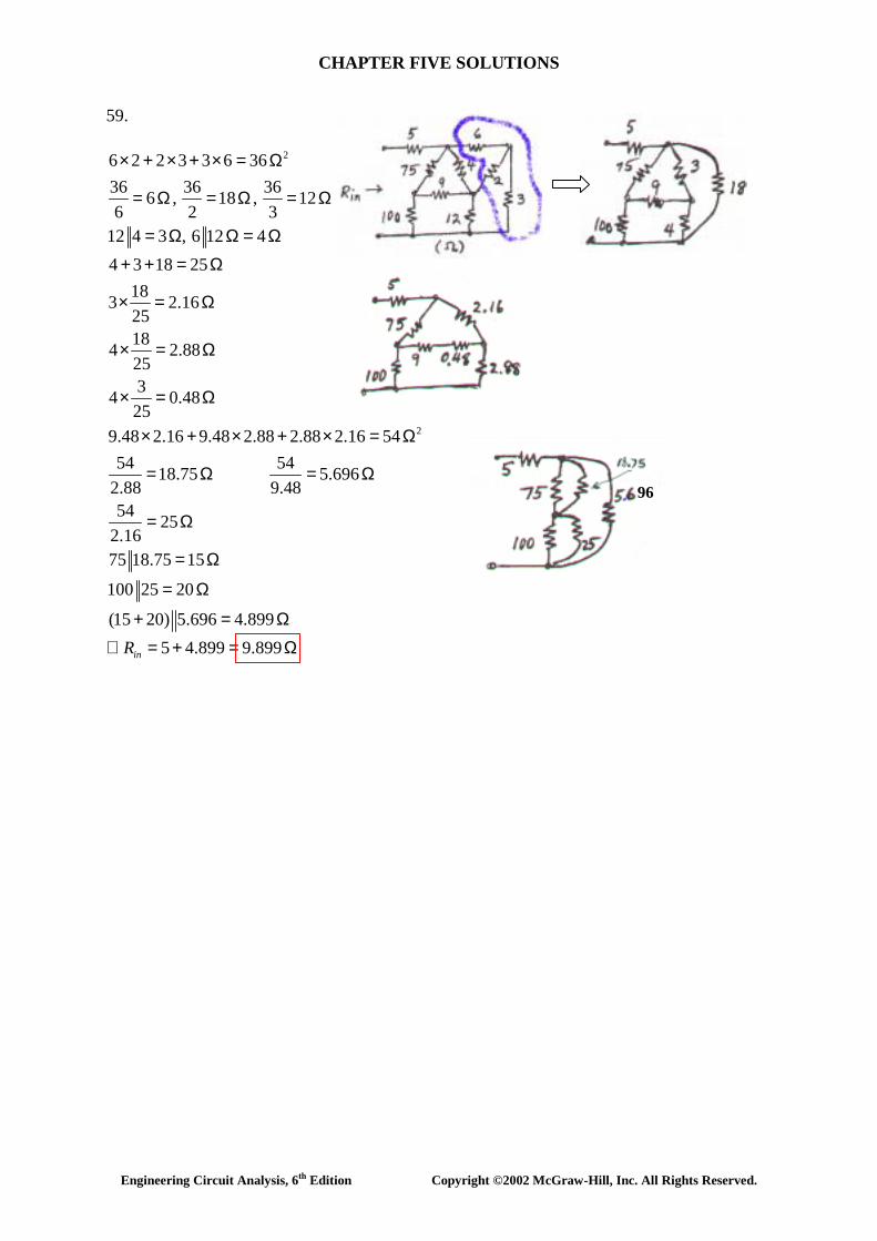
59.

2

2

6 2 2 3 3 6 3636 36 366 , 18 , 126 2 3

12 4 3 , 6 12 44 3 18 25

183 2.1625184 2.882534 0.4825

9.48 2.16 9.48 2.88 2.88 2.16 5454 5418.75 5.696

2.88 9.4854 25

2.1675 18.75 15

100 25 20

(15 20) 5.696

× + × + × = Ω

= Ω = Ω = Ω

= Ω Ω = Ω+ + = Ω

× = Ω

× = Ω

× = Ω

× + × + × = Ω

= Ω = Ω

= Ω

= Ω

= Ω

+ = 4.8995 4.899 9.899

Ω∴ = + = ΩinR

96



60. We begin by converting the ∆-connected network consisting of the 4-, 6-, and 3-Ω resistors to an equivalent Y-connected network:

1

2

3

6 4 3 136 4 1.846134 3 923.1m13

3 6 1.38513

= + + = Ω×= = = Ω

×= = = Ω

×= = = Ω

A B

B C

C A

DR RR

DR RR

DR RR

D

Then network becomes: Then we may write

12 [13.846 (19.385 6.9231)]7.347

= += Ω

inR

RA RB

RC

1.846 Ω 0.9231 Ω

1.385 Ω



0.5 0.5 0.25

61. Next, we convert the Y-connected network on the left to a ∆-connected network:

21 0.5 0.5 2 2 1 3.5× + × + × = Ω

3.5 70.53.5 1.752

3.5 3.51

= = Ω

= = Ω

= = Ω

A

B

C

R

R

R

After this procedure, we have a 3.5-Ω resistor in parallel with the 2.5-Ω resistor. Replacing them with a 1.458-Ω resistor, we may redraw the circuit: This circuit may be easily analysed to find:

1

2

3

1 1 2 41 2 1

4 22 1 1

4 21 1 0.25

4

+ + = Ω×= = Ω

×= = Ω

×= = Ω

R

R

R

12 1.458 5.454 V1.75 1.4580.25 1.458 1.751.045

×= =+

= += Ω

oc

TH

V

R

7

1.75 0.25

1.458



62. We begin by converting the Y-network to a ∆-connected network:

21.1 1.1 1.1 33 313 313 31

= + + = Ω

= = Ω

= = Ω

= = Ω

A

B

C

N

R

R

R

Next, we note that 1 3 0.75= Ω , and hence have a simple ∆-network. This is easily converted to a Y-connected network:

1

2

3

0.75 3 3 6.750.75 3 0.3333

6.753 3 1.3336.753 0.75 0.3333

6.75

+ + = Ω×= = Ω

×= = Ω

×= = Ω

R

R

R

1.333 0.33331.667

1/ 311/ 3 1 1/ 3

1 11 3 1 50.2A200mA

= += Ω

= = ×+ +

= =+ +

==

N

N SC

R

I I

33

3 Ω

1 A

Analysing this final circuit,



63. Since 1 V appears across the resistor associated with I1, we know that I1 = 1 V/ 10 Ω = 100 mA. From the perspective of the open terminals, the 10-Ω resistor in parallel with the voltage source has no influence if we replace the “dependent” source with a fixed 0.5-A source:

Then, we may write:

-1 + (10 + 10 + 10) ia – 10 (0.5) = 0 so that ia = 200 mA. We next find that VTH = Vab = 10(-0.5) + 10(ia – 0.5) + 10(-0.5) = -13 V. To determine RTH, we first recognise that with the 1-V source shorted, I1 = 0 and

hence the dependent current source is dead. Thus, we may write RTH from inspection:

RTH = 10 + 10 + 10 || 20 = 26.67 Ω.

0.5 A



64. (a) We begin by splitting the 1-kΩ resistor into two 500-Ω resistors in series. We then have two related Y-connected networks, each with a 500-Ω resistor as a leg. Converting those networks into ∆-connected networks,

Σ = (17)(10) + (1)(4) + (4)(17) = 89×106 Ω2

89/0.5 = 178 kΩ; 89/ 17 = 5.236 kΩ; 89/4 = 22.25 kΩ

Following this conversion, we find that we have two 5.235 kΩ resistors in parallel, and a 178-kΩ resistor in parallel with the 4-kΩ resistor. Noting that 5.235 k || 5.235 k = 2.618 kΩ and 178 k || 4 k = 3.912 kΩ, we may draw the circuit as:

We next attack the Y-connected network in the center:

Σ = (22.25)(22.25) + (22.25)(2.618) + (2.618)(22.25) = 611.6×106 Ω2

611.6/ 22.25 = 27.49 kΩ; 611.6/ 2.618 = 233.6 kΩ

Noting that 178 k || 27.49 k = 23.81 kΩ and 27.49 || 3.912 = 3.425 kΩ, we are left with a simple ∆-connected network. To convert this to the requested Y-network,

Σ = 23.81 + 233.6 + 3.425 = 260.8 kΩ

(23.81)(233.6)/ 260.8 = 21.33 kΩ (233.6)(3.425)/ 260.8 = 3.068 kΩ (3.425)(23.81)/ 260.8 = 312.6 Ω

178 kΩ

233.6 kΩ

27.49 kΩ 27.49 kΩ 3.912 kΩ

312.6 Ω

21.33 kΩ 3.068 kΩ

(b)



65. (a) Although this network may be simplified, it is not possible to replace it with a three-resistor equivalent.

(b) See (a).



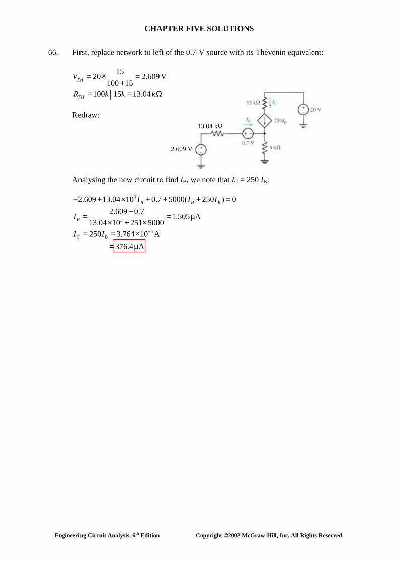
66. First, replace network to left of the 0.7-V source with its Thévenin equivalent:

1520 2.609V

100 15100 15 13.04

= × =+

= = Ω

TH

TH

V

R k k k

Redraw: Analysing the new circuit to find IB, we note that IC = 250 IB:

3

3

4

2.609 13.04 10 0.7 5000( 250 ) 02.609 0.7 1.505 A

13.04 10 251 5000250 3.764 10 A

376.4 A

−

− + × + + + =−= = µ

× + ×= = ×

= µ

B B B

B

C B

I I I

I

I I

2.609 V

13.04 kΩ



67. (a) Define a nodal voltage V1 at the top of the current source IS, and a nodal voltage V2 at the top of the load resistor RL. Since the load resistor can safely dissipate 1 W, and we know that

PRL = 1000V2

2

then V 31.62 Vmax2 = . This corresponds to a load resistor (and hence lamp) current

of 32.62 mA, so we may treat the lamp as a 10.6-Ω resistor. Proceeding with nodal analysis, we may write:

IS = V1/ 200 + (V1 – 5 Vx)/ 200 [1]

0 = V2/ 1000 + (V2 – 5 Vx)/ 10.6 [2]

Vx = V1 – 5 Vx or Vx = V1/ 6 [3] Substituting Eq. [3] into Eqs. [1] and [2], we find that

7 V1 = 1200 IS [1] -5000 V1 + 6063.6 V2 = 0 [2]

Substituting V 31.62 Vmax2 = into Eq. [2] then yields V1 = 38.35 V, so that

IS| max = (7)(38.35)/ 1200 = 223.7 mA. (b) PSpice verification. The lamp current does not exceed 36 mA in the range of operation allowed (i.e. a load power of < 1 W.) The simulation result shows that the load will dissipate slightly more than 1 W for a source current magnitude of 224 mA, as predicted by hand analysis.



68. Short out all but the source operating at 104 rad/s, and define three clockwise mesh currents i1, i2, and i3 starting with the left-most mesh. Then

608 i1 – 300 i2 = 3.5 cos 104 t [1] -300 i1 + 316 i2 – 8 i3 = 0 [2] -8 i2 + 322 i3 = 0 [3] Solving, we find that i1(t) = 10.84 cos 104 t mA i2(t) = 10.29 cos 104 t mA i3(t) = 255.7 cos 104 t µA Next, short out all but the 7 sin 200t V source, and and define three clockwise mesh

currents ia, ib, and ic starting with the left-most mesh. Then 608 ia – 300 ib = -7 sin 200t [1] -300 ia + 316 ib – 8 ic = 7 sin 200t [2] -8 ib + 322 ic = 0 [3] Solving, we find that ia(t) = -1.084 sin 200t mA ib(t) = 21.14 sin 200t mA ic(t) = 525.1 sin 200t µA Next, short out all but the source operating at 103 rad/s, and define three clockwise

mesh currents iA, iB, and iC starting with the left-most mesh. Then 608 iA – 300 iB = 0 [1] -300 iA + 316 iB – 8 iC = 0 [2] -8 iB + 322 iC = -8 cos 104 t [3]

Solving, we find that iA(t) = -584.5 cos 103 t µA iB(t) = -1.185 cos 103 t mA iC(t) = -24.87 cos 103 t mA

We may now compute the power delivered to each of the three 8-Ω speakers: p1 = 8[i1 + ia + iA]2 = 8[10.84×10-3 cos 104 t -1.084×10-3 sin 200t -584.5×10-6 cos 103 t]2 p2 = 8[i2 + ib + iB]2 = 8[10.29×10-3 cos 104 t +21.14×10-3 sin 200t –1.185×10-3 cos 103 t]2 p3 = 8[i3 + ic + iC]2 = 8[255.7×10-6 cos 104 t +525.1×10-6 sin 200t –24.87×10-3 cos 103 t]2



69. Replacing the DMM with a possible Norton equivalent (a 1-MΩ resistor in parallel with a 1-A source):

We begin by noting that 33 Ω || 1 MΩ ≈ 33 Ω. Then,

0 = (V1 – Vin)/ 33 + V1/ 275×103 [1] and 1 - 0.7 V1 = Vin/ 106 + Vin/ 33×103 + (Vin – V1)/ 33 [2] Simplifying and collecting terms, (275×103 + 33) V1 - 275×103 Vin = 0 [1] 22.1 V1 + 1.001 Vin = 33 [2] Solving, we find that Vin = 1.429 V; in other words, the DMM sees 1.429 V across its

terminals in response to the known current of 1 A it’s supplying. It therefore thinks that it is connected to a resistance of 1.429 Ω.

1 A

Vin



70. We know that the resistor R is absorbing maximum power. We might be tempted to say that the resistance of the cylinder is therefore 10 Ω, but this is wrong: The larger we make the cylinder resistance, the small the power delivery to R:

PR = 10 i2 = 10 2

10 120

+cylinderR

Thus, if we are in fact delivering the maximum possible power to the resistor from the 120-V source, the resistance of the cylinder must be zero. This corresponds to a temperature of absolute zero using the equation given.



71. We note that the buzzer draws 15 mA at 6 V, so that it may be modeled as a 400-Ω

resistor. One possible solution of many, then, is: Note: construct the 18-V source from 12 1.5-V batteries in series, and the two 400-Ω

resistors can be fabricated by soldering 400 1-Ω resistors in series, although there’s probably a much better alternative…



72. To solve this problem, we need to assume that “45 W” is a designation that applies

when 120 Vac is applied directly to a particular lamp. This corresponds to a current draw of 375 mA, or a light bulb resistance of 120/ 0.375 = 320 Ω.

Original wiring scheme New wiring scheme

In the original wiring scheme, Lamps 1 & 2 draw (40)2 / 320 = 5 W of power each, and Lamp 3 draws (80)2 / 320 = 20 W of power. Therefore, none of the lamps is running at its maximum rating of 45 W. We require a circuit which will deliver the same intensity after the lamps are reconnected in a ∆ configuration. Thus, we need a total of 30 W from the new network of lamps.

There are several ways to accomplish this, but the simplest may be to just use one 120-Vac source connected to the left port in series with a resistor whose value is chosen to obtain 30 W delivered to the three lamps.

In other words,

30 320

213.3Rs213.3 06

2 320

213.3Rs213.3 120

22

=

++

+

Solving, we find that we require Rs = 106.65 Ω, as confirmed by the PSpice simulation below, which shows that both wiring configurations lead to one lamp with 80-V across it, and two lamps with 40 V across each.

3



73. • Maximum current rating for the LED is 35 mA. • Its resistance can vary between 47 and 117 Ω. • A 9-V battery must be used as a power source. • Only standard resistance values may be used.

One possible current-limiting scheme is to connect a 9-V battery in series with a

resistor Rlimiting and in series with the LED. From KVL,

ILED = LEDlimiting R R

9+

The maximum value of this current will occur at the minimum LED resistance, 47 Ω. Thus, we solve

35×10-3 = 47 R

9

limiting +

to obtain Rlimiting ≥ 210.1 Ω to ensure an LED current of less than 35 mA. This is not a standard resistor value, however, so we select

Rlimiting = 220 Ω.

Documents

CHAPTER FIVE SOLUTIONS - Innovative Learning Solutions ... · PDF fileCHAPTER FIVE SOLUTIONS Engineering Circuit Analysis, 6th Edition Copyright ©2002 McGraw-Hill, Inc. All Rights