CHAPTER - IV ANALYSIS OF CAPITAL STRUCTURE OF SELECTED UNITS

87

CHAPTER - IV

ANALYSIS OF CAPITAL STRUCTURE OF SELECTED UNITS

4.1 INTRODUCTION

The most crucial decision of any company is involved in formulation of its

appropriate capital structure. Capital structure ordinarily implies the proportion of

debt and equity in the total capital of a company. The best design or structure of the

capital of a company obviously helps the management to achieve its ultimate

objectives of minimizing overall cost of capital, and also maximizing the value of the

firm. It is thus apparent that the design of the capital structure of a company may have

a bearing on the profitability of the company.

Ordinarily, increase in debt in the capital structure i.e., improvement of debt-equity

ratio implies greater amount of interest payment than before. So, the company must

have to be sure enough of getting steady return so as to bear the additional burden of

interest. Actually, a negative correlation should always exist between cost of capital

and profitability. So, increase in cost of capital means decrease in profitability.

The present study is undertaken to find out the relationship between the capital

structure and profitability and to analyze the capital structures of the selected

pharmaceutical and engineering units.1

The short- term creditors, like bankers and suppliers of raw material, are more

concerned with the firm’s current debt-paying ability. On the other hand, long-term

creditors, like debenture holders, financial institutions, etc. are more concerned with

the firm’s long-term financial strength. In fact, a firm should have a strong short as

well as long-term financial position. To judge the long-term financial position of the

firm, financial leverage or capital structure ratios are calculated.

Leverage ratios are calculated to measure the financial risk and the firm’s ability of

using debt to shareholder’s advantage. Leverage ratios may be calculated from the

balance sheet items to determine the proportion of debt in total financing. They are

also computed from the profit and loss items by determining the extent to which

operating profits are sufficient to cover the fixed charges.2

88

These ratios help in ascertaining the long-term solvency of a firm which depends

basically on three factors:

1. Whether the firm has adequate resources to meet its long-term funds

requirements;

2. Whether the firm has used an appropriate debt-equity mix to raise long-term

funds;

3. Whether the firm earns enough to pay interest and installment of long-term loans

in time. 3

4.2 LEVERAGE RATIOS OF SELECTED ENGINEERING UNITS

4.2.1 Debt-Equity Ratio

The debt-equity ratio is determined to ascertain the soundness of the long-term

financial policies of the company. This ratio indicates the relationship between loan

funds and net worth of the company, which is known as gearing. A debt-equity ratio

of 2:1 is the norm accepted by financial institutions for financing of projects. Higher

debt-equity ratio may be permitted for highly capital intensive industries like

petrochemicals, fertilizers, etc. A debt-equity ratio which shows a declining trend over

the years is usually taken as a positive sign reflecting on increasing cash accrual and

debt repayment.

Debt-equity ratio can be calculated as:

Debt-equity ratio = Long-Term Debt

Shareholders Funds

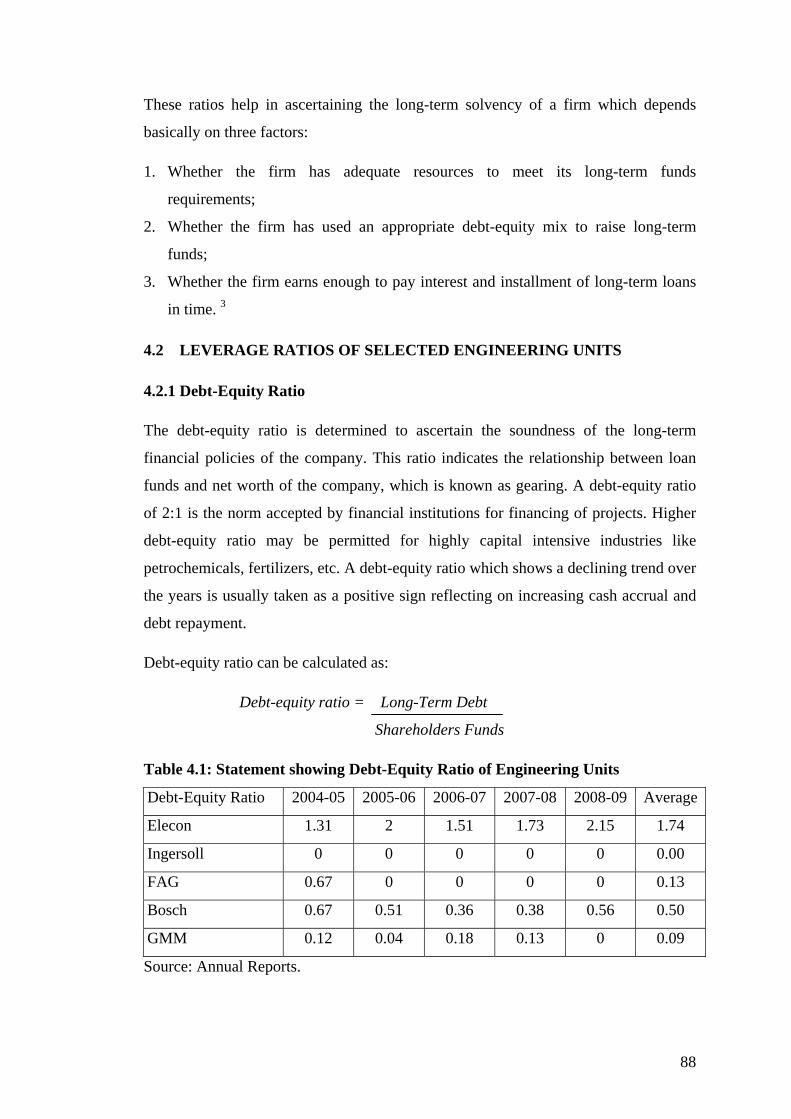
Table 4.1: Statement showing Debt-Equity Ratio of Engineering Units

Debt-Equity Ratio 2004-05 2005-06 2006-07 2007-08 2008-09 Average

Elecon 1.31 2 1.51 1.73 2.15 1.74

Ingersoll 0 0 0 0 0 0.00

FAG 0.67 0 0 0 0 0.13

Bosch 0.67 0.51 0.36 0.38 0.56 0.50

GMM 0.12 0.04 0.18 0.13 0 0.09

Source: Annual Reports.

89

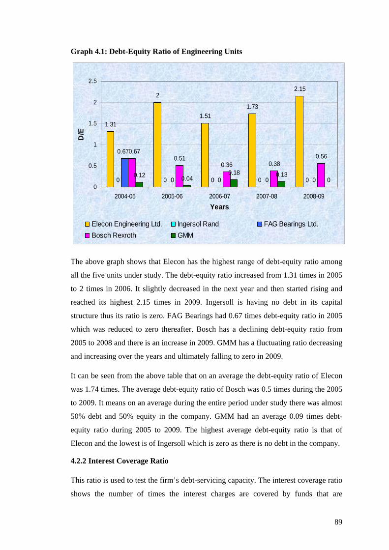
Graph 4.1: Debt-Equity Ratio of Engineering Units

1.31

2

1.511.73

2.15

0 0 0 0 00 0 0 0

0.510.36 0.38

0.56

0.12 0.040.18 0.13

0

0.670.67

0

0.5

1

1.5

2

2.5

2004-05 2005-06 2006-07 2007-08 2008-09

Years

D/E

Elecon Engineering Ltd. Ingersol Rand FAG Bearings Ltd.Bosch Rexroth GMM

The above graph shows that Elecon has the highest range of debt-equity ratio among

all the five units under study. The debt-equity ratio increased from 1.31 times in 2005

to 2 times in 2006. It slightly decreased in the next year and then started rising and

reached its highest 2.15 times in 2009. Ingersoll is having no debt in its capital

structure thus its ratio is zero. FAG Bearings had 0.67 times debt-equity ratio in 2005

which was reduced to zero thereafter. Bosch has a declining debt-equity ratio from

2005 to 2008 and there is an increase in 2009. GMM has a fluctuating ratio decreasing

and increasing over the years and ultimately falling to zero in 2009.

It can be seen from the above table that on an average the debt-equity ratio of Elecon

was 1.74 times. The average debt-equity ratio of Bosch was 0.5 times during the 2005

to 2009. It means on an average during the entire period under study there was almost

50% debt and 50% equity in the company. GMM had an average 0.09 times debt-

equity ratio during 2005 to 2009. The highest average debt-equity ratio is that of

Elecon and the lowest is of Ingersoll which is zero as there is no debt in the company.

4.2.2 Interest Coverage Ratio

This ratio is used to test the firm’s debt-servicing capacity. The interest coverage ratio

shows the number of times the interest charges are covered by funds that are

90

ordinarily available for their payment. Since taxes are computed after interest, interest

coverage is calculated in relation to before tax earnings. This ratio indicates the extent

to which earnings may fall without causing any embarrassment to the firm regarding

the payment of the interest charges. A higher ratio is desirable; but too high a ratio

indicates that the firm is very conservative in using debt, and that it is not using credit

to the best advantage of shareholders. A lower ratio indicates excessive use of debt, or

inefficient operations. 4

The interest coverage ratio is computed as:

Interest Coverage Ratio = EBIT Interest

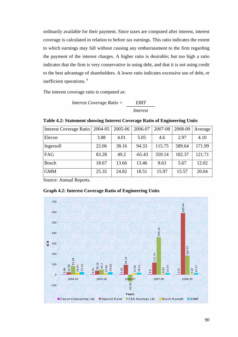
Table 4.2: Statement showing Interest Coverage Ratio of Engineering Units

Interest Coverage Ratio 2004-05 2005-06 2006-07 2007-08 2008-09 Average

Elecon 3.88 4.01 5.05 4.6 2.97 4.10

Ingersoll 22.06 38.16 94.33 115.75 589.64 171.99

FAG 83.28 49.2 -65.43 359.14 182.37 121.71

Bosch 18.67 13.66 13.46 8.63 5.67 12.02

GMM 25.35 24.82 18.51 15.97 15.57 20.04


Graph 4.2: Interest Coverage Ratio of Engineering Units

3.88

4.01

5.05

4.6

2.9722.06

38.16 94

.33

115.75

589.64

83.28

49.2

‐65.43

359.14

182.37

18.67

13.66

13.46

8.63

5.6725

.35

24.82

18.51

15.97

15.57

‐100

0

100

200

300

400

500

600

700

2004‐05 2005‐06 2006‐07 2007‐08 2008‐09

Years

ICR

E lecon E ngineering L td. Ingersol R and FAG Bearings L td. Bosch R exroth GMM

91

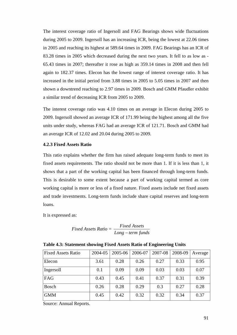
The interest coverage ratio of Ingersoll and FAG Bearings shows wide fluctuations

during 2005 to 2009. Ingersoll has an increasing ICR, being the lowest at 22.06 times

in 2005 and reaching its highest at 589.64 times in 2009. FAG Bearings has an ICR of

83.28 times in 2005 which decreased during the next two years. It fell to as low as -

65.43 times in 2007; thereafter it rose as high as 359.14 times in 2008 and then fell

again to 182.37 times. Elecon has the lowest range of interest coverage ratio. It has

increased in the initial period from 3.88 times in 2005 to 5.05 times in 2007 and then

shown a downtrend reaching to 2.97 times in 2009. Bosch and GMM Pfaudler exhibit

a similar trend of decreasing ICR from 2005 to 2009.

The interest coverage ratio was 4.10 times on an average in Elecon during 2005 to

2009. Ingersoll showed an average ICR of 171.99 being the highest among all the five

units under study, whereas FAG had an average ICR of 121.71. Bosch and GMM had

an average ICR of 12.02 and 20.04 during 2005 to 2009.

4.2.3 Fixed Assets Ratio

This ratio explains whether the firm has raised adequate long-term funds to meet its

fixed assets requirements. The ratio should not be more than 1. If it is less than 1, it

shows that a part of the working capital has been financed through long-term funds.

This is desirable to some extent because a part of working capital termed as core

working capital is more or less of a fixed nature. Fixed assets include net fixed assets

and trade investments. Long-term funds include share capital reserves and long-term

loans.

It is expressed as:

Fixed Assets Ratio = fundstermLong

AssetsFixed−

Table 4.3: Statement showing Fixed Assets Ratio of Engineering Units

Fixed Assets Ratio 2004-05 2005-06 2006-07 2007-08 2008-09 Average

Elecon 3.61 0.28 0.26 0.27 0.33 0.95

Ingersoll 0.1 0.09 0.09 0.03 0.03 0.07

FAG 0.43 0.45 0.41 0.37 0.31 0.39

Bosch 0.26 0.28 0.29 0.3 0.27 0.28

GMM 0.45 0.42 0.32 0.32 0.34 0.37


92

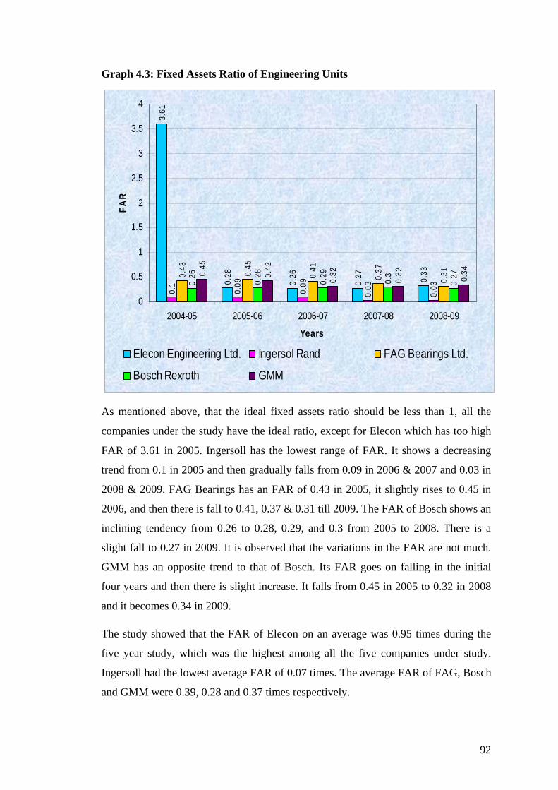
Graph 4.3: Fixed Assets Ratio of Engineering Units

3.61

0.28

0.26

0.27 0.33

0.1

0.09

0.09

0.03

0.03

0.43 0.45

0.41

0.37

0.31

0.26

0.28

0.29

0.3

0.270.

45

0.42

0.32

0.32 0.34

0

0.5

1

1.5

2

2.5

3

3.5

4

2004-05 2005-06 2006-07 2007-08 2008-09

Years

FAR

Elecon Engineering Ltd. Ingersol Rand FAG Bearings Ltd.

Bosch Rexroth GMM

As mentioned above, that the ideal fixed assets ratio should be less than 1, all the

companies under the study have the ideal ratio, except for Elecon which has too high

FAR of 3.61 in 2005. Ingersoll has the lowest range of FAR. It shows a decreasing

trend from 0.1 in 2005 and then gradually falls from 0.09 in 2006 & 2007 and 0.03 in

2008 & 2009. FAG Bearings has an FAR of 0.43 in 2005, it slightly rises to 0.45 in

2006, and then there is fall to 0.41, 0.37 & 0.31 till 2009. The FAR of Bosch shows an

inclining tendency from 0.26 to 0.28, 0.29, and 0.3 from 2005 to 2008. There is a

slight fall to 0.27 in 2009. It is observed that the variations in the FAR are not much.

GMM has an opposite trend to that of Bosch. Its FAR goes on falling in the initial

four years and then there is slight increase. It falls from 0.45 in 2005 to 0.32 in 2008

and it becomes 0.34 in 2009.

The study showed that the FAR of Elecon on an average was 0.95 times during the

five year study, which was the highest among all the five companies under study.

Ingersoll had the lowest average FAR of 0.07 times. The average FAR of FAG, Bosch

and GMM were 0.39, 0.28 and 0.37 times respectively.

93

4.2.4 Statistical Analysis of Engineering Units

DEQR & EPS

For studying the trend between debt-equity ratio and the earnings per share, curve fit

has been used.

Table 4.4: Table showing the model summary of DEQR & EPS of Engineering

Units

Model Summary

R R Square Adjusted R Square Std. Error of the Estimate

.287 .082 .043 .737

The independent variable is DEQR.

Source: Self tabulated.

As mentioned above DEQR is the independent variable whereas EPS is the dependent

variable.

The equation applied is: y = a + bx

The above table shows that R=0.287 which means that the correlation between x and

y, i.e. DEQR and EPS is not so strong. Both are partially positively related.

In the above study, the growth model as well as exponential model both gives the

same result.

ANOVA has been used to test the mean values of different variables. Two hypotheses

are framed.

H0 = There is a significant difference between the mean values of all variable values.

H1 = There is no significant difference between the mean values of all variable values.

Table 4.5: Statement of ANOVA of DEQR & EPS of Engineering Units

Sum of Squares df Mean Square F Sig.

Regression 1.121 1 1.121 2.066 .164

Residual 12.485 23 .543

Total 13.607 24



The above table shows that F>Sig. which means that H0 is rejected. It means that

there is a significant difference between means of all the variable values.

94

T-test has been conducted to find out the correlation between DEQR and EPS.

Table 4.6: Test of Significance of Correlation Coefficients between DEQR & EPS

of Engineering Units

Coefficients

Unstandardized

Coefficients

Standardized

Coefficients

B Std. Error Beta

t Sig.

DEQR -.314 .219 -.287 -1.437 .164

(Constant) 3.343 .183 18.313 .000

The dependent variable is EPS.


It shows whether there is a significant difference between the mean values of the

variables.

H0 = There is a significant difference between the mean values of DEQR and EPS.

H1 = There is no significant difference between the mean values of DEQR and EPS.

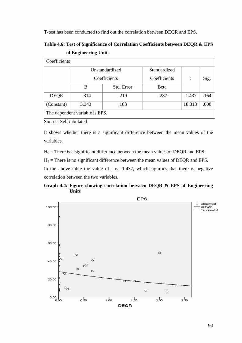
In the above table the value of t is -1.437, which signifies that there is negative

correlation between the two variables.

Graph 4.4: Figure showing correlation between DEQR & EPS of Engineering Units

95

The graph plotted from the above study shows that as DEQR increases, EPS

decreases. But it is not so for all the observations made under the study.

DEQR & FAR

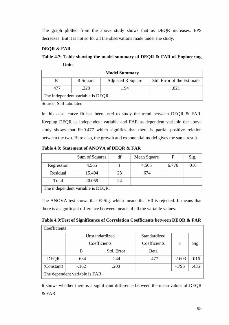
Table 4.7: Table showing the model summary of DEQR & FAR of Engineering

Units

Model Summary R R Square Adjusted R Square Std. Error of the Estimate

.477 .228 .194 .821



In this case, curve fit has been used to study the trend between DEQR & FAR.

Keeping DEQR as independent variable and FAR as dependent variable the above

study shows that R=0.477 which signifies that there is partial positive relation

between the two. Here also, the growth and exponential model gives the same result.

Table 4.8: Statement of ANOVA of DEQR & FAR


Regression 4.565 1 4.565 6.776 .016

Residual 15.494 23 .674

Total 20.059 24


The ANOVA test shows that F>Sig. which means that H0 is rejected. It means that

there is a significant difference between means of all the variable values.

Table 4.9:Test of Significance of Correlation Coefficients between DEQR & FAR

Coefficients

Unstandardized Coefficients

Standardized Coefficients

B Std. Error Beta

t Sig.

DEQR -.634 .244 -.477 -2.603 .016

(Constant) -.162 .203 -.795 .435

The dependent variable is FAR.

It shows whether there is a significant difference between the mean values of DEQR

& FAR.

96

H0 = There is a significant difference between the mean values of DEQR and FAR.

H1 = There is no significant difference between the mean values of DEQR and FAR.



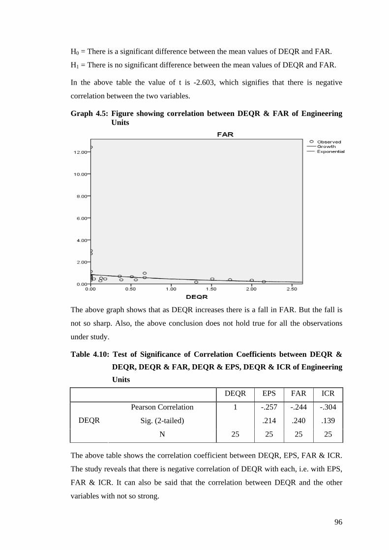
Graph 4.5: Figure showing correlation between DEQR & FAR of Engineering Units

The above graph shows that as DEQR increases there is a fall in FAR. But the fall is

not so sharp. Also, the above conclusion does not hold true for all the observations

under study.

Table 4.10: Test of Significance of Correlation Coefficients between DEQR & DEQR, DEQR & FAR, DEQR & EPS, DEQR & ICR of Engineering Units

DEQR EPS FAR ICR

Pearson Correlation 1 -.257 -.244 -.304

Sig. (2-tailed) .214 .240 .139 DEQR

N 25 25 25 25

The above table shows the correlation coefficient between DEQR, EPS, FAR & ICR.

The study reveals that there is negative correlation of DEQR with each, i.e. with EPS,

FAR & ICR. It can also be said that the correlation between DEQR and the other

variables with not so strong.

97

Table 4.11: Statement showing linear & exponential relation of DEQR with EPS,

FAR & ICR of Engineering Units

EPS FAR ICR

Linear Exponential Linear Exponential Linear Exponential

Constant 50.107 *

(6.697)

67.168

(1.33)

0.286*

(1.725)

0.207*

(4.446)

188.54*

(4.045)

----

DEQR -22.007*

(3.689)

-1.5*

(2.5)

0.257

(1.298)

0.437

(1.622)

-128.37*

(4.737)

-----

*indicates significant value at 5% level of significance.

From the above table it is observed that EPS, FAR and ICR have no linear effect of

DEQR but FAR is affected exponentially by DEQR and the model gives significant

results. It indicates that 1 unit rise in DEQR results in 43% rise in FAR exponentially.

4.3 LEVERAGE RATIOS OF SELECTED PHARMACEUTICAL

COMPANIES

4.3.1 Debt-Equity Ratio

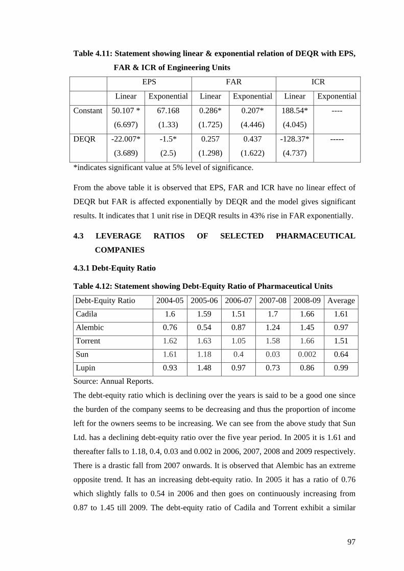
Table 4.12: Statement showing Debt-Equity Ratio of Pharmaceutical Units

Debt-Equity Ratio 2004-05 2005-06 2006-07 2007-08 2008-09 Average

Cadila 1.6 1.59 1.51 1.7 1.66 1.61

Alembic 0.76 0.54 0.87 1.24 1.45 0.97

Torrent 1.62 1.63 1.05 1.58 1.66 1.51

Sun 1.61 1.18 0.4 0.03 0.002 0.64

Lupin 0.93 1.48 0.97 0.73 0.86 0.99


The debt-equity ratio which is declining over the years is said to be a good one since

the burden of the company seems to be decreasing and thus the proportion of income

left for the owners seems to be increasing. We can see from the above study that Sun

Ltd. has a declining debt-equity ratio over the five year period. In 2005 it is 1.61 and

thereafter falls to 1.18, 0.4, 0.03 and 0.002 in 2006, 2007, 2008 and 2009 respectively.

There is a drastic fall from 2007 onwards. It is observed that Alembic has an extreme

opposite trend. It has an increasing debt-equity ratio. In 2005 it has a ratio of 0.76

which slightly falls to 0.54 in 2006 and then goes on continuously increasing from

0.87 to 1.45 till 2009. The debt-equity ratio of Cadila and Torrent exhibit a similar

98

trend. There is a slight fall in the ratio in the middle period of study and then it

ultimately grows by the end of the period. Lupin shows a better debt-equity ratio.

There is a rise in the ratio from 0.93 in 2005 to 1.48 in 2006 but thereafter it falls from

0.97 to 0.73 in 2008 with a slight rise to 0.86 in 2009.

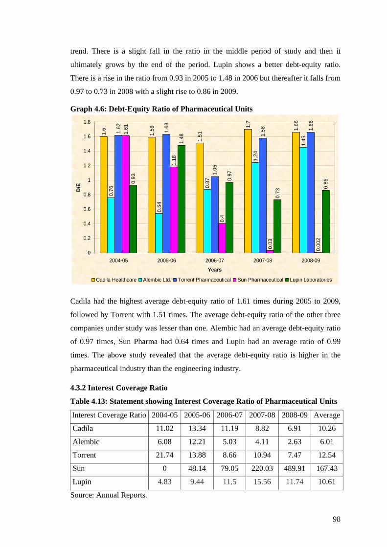
Graph 4.6: Debt-Equity Ratio of Pharmaceutical Units 1.

6

1.59

1.51

1.7

1.66

0.76

0.54

0.87

1.24

1.45

1.62

1.63

1.05

1.58 1.

66

1.61

1.18

0.4

0.03

0.00

2

0.93

1.48

0.97

0.73

0.86

0

0.2

0.4

0.6

0.8

1

1.2

1.4

1.6

1.8

2004-05 2005-06 2006-07 2007-08 2008-09

Years

D/E

Cadila Healthcare Alembic Ltd. Torrent Pharmaceutical Sun Pharmaceutical Lupin Laboratories

Cadila had the highest average debt-equity ratio of 1.61 times during 2005 to 2009,

followed by Torrent with 1.51 times. The average debt-equity ratio of the other three

companies under study was lesser than one. Alembic had an average debt-equity ratio

of 0.97 times, Sun Pharma had 0.64 times and Lupin had an average ratio of 0.99

times. The above study revealed that the average debt-equity ratio is higher in the

pharmaceutical industry than the engineering industry.

4.3.2 Interest Coverage Ratio

Table 4.13: Statement showing Interest Coverage Ratio of Pharmaceutical Units

Interest Coverage Ratio 2004-05 2005-06 2006-07 2007-08 2008-09 Average

Cadila 11.02 13.34 11.19 8.82 6.91 10.26

Alembic 6.08 12.21 5.03 4.11 2.63 6.01

Torrent 21.74 13.88 8.66 10.94 7.47 12.54

Sun 0 48.14 79.05 220.03 489.91 167.43

Lupin 4.83 9.44 11.5 15.56 11.74 10.61


99

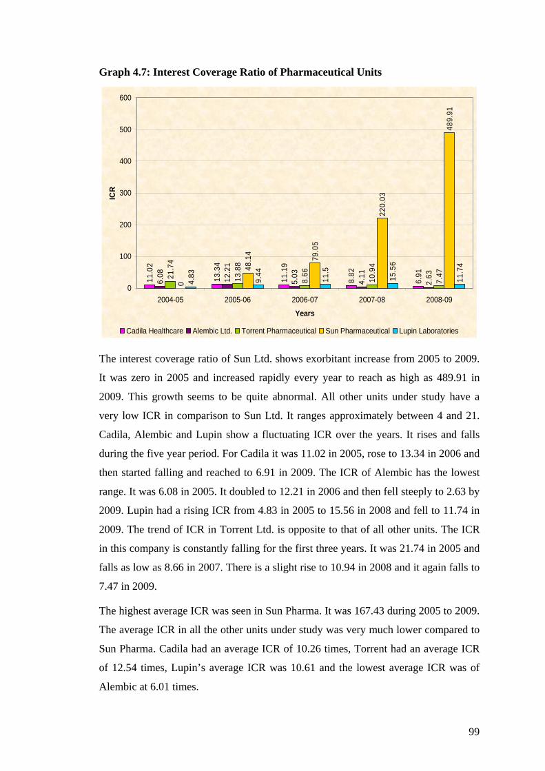
Graph 4.7: Interest Coverage Ratio of Pharmaceutical Units

11.0

2

13.3

4

11.1

9

8.82

6.91

6.08 12

.21

5.03

4.11

2.6321

.74

13.8

8

8.66

10.9

4

7.47

0

48.1

4

79.0

5

220.

03

489.

91

4.83 9.44

11.5

15.5

6

11.7

4

0

100

200

300

400

500

600

2004-05 2005-06 2006-07 2007-08 2008-09

Years

ICR

Cadila Healthcare Alembic Ltd. Torrent Pharmaceutical Sun Pharmaceutical Lupin Laboratories

The interest coverage ratio of Sun Ltd. shows exorbitant increase from 2005 to 2009.

It was zero in 2005 and increased rapidly every year to reach as high as 489.91 in

2009. This growth seems to be quite abnormal. All other units under study have a

very low ICR in comparison to Sun Ltd. It ranges approximately between 4 and 21.

Cadila, Alembic and Lupin show a fluctuating ICR over the years. It rises and falls

during the five year period. For Cadila it was 11.02 in 2005, rose to 13.34 in 2006 and

then started falling and reached to 6.91 in 2009. The ICR of Alembic has the lowest

range. It was 6.08 in 2005. It doubled to 12.21 in 2006 and then fell steeply to 2.63 by

2009. Lupin had a rising ICR from 4.83 in 2005 to 15.56 in 2008 and fell to 11.74 in

2009. The trend of ICR in Torrent Ltd. is opposite to that of all other units. The ICR

in this company is constantly falling for the first three years. It was 21.74 in 2005 and

falls as low as 8.66 in 2007. There is a slight rise to 10.94 in 2008 and it again falls to

7.47 in 2009.

The highest average ICR was seen in Sun Pharma. It was 167.43 during 2005 to 2009.

The average ICR in all the other units under study was very much lower compared to

Sun Pharma. Cadila had an average ICR of 10.26 times, Torrent had an average ICR

of 12.54 times, Lupin’s average ICR was 10.61 and the lowest average ICR was of

Alembic at 6.01 times.

100

If we compare the ICR of the pharmaceutical and engineering units under study it was

seen that the average ICR during 2005 to 2009 of pharmaceutical industry was higher

than the engineering industry but the range of overall average of the engineering units

under study was higher than the pharmaceutical industry.

4.3.3 Fixed Assets Ratio

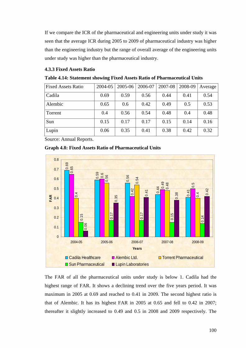
Table 4.14: Statement showing Fixed Assets Ratio of Pharmaceutical Units

Fixed Assets Ratio 2004-05 2005-06 2006-07 2007-08 2008-09 Average

Cadila 0.69 0.59 0.56 0.44 0.41 0.54

Alembic 0.65 0.6 0.42 0.49 0.5 0.53

Torrent 0.4 0.56 0.54 0.48 0.4 0.48

Sun 0.15 0.17 0.17 0.15 0.14 0.16

Lupin 0.06 0.35 0.41 0.38 0.42 0.32


Graph 4.8: Fixed Assets Ratio of Pharmaceutical Units

0.69

0.59

0.56

0.44

0.41

0.65

0.6

0.42

0.49 0.5

0.4

0.56

0.54

0.48

0.4

0.17

0.17

0.14

0.06

0.35

0.41

0.38 0.

42

0.15

0.15

0

0.1

0.2

0.3

0.4

0.5

0.6

0.7

0.8

2004-05 2005-06 2006-07 2007-08 2008-09

Years

FAR

Cadila Healthcare Alembic Ltd. Torrent PharmaceuticalSun Pharmaceutical Lupin Laboratories

The FAR of all the pharmaceutical units under study is below 1. Cadila had the

highest range of FAR. It shows a declining trend over the five years period. It was

maximum in 2005 at 0.69 and reached to 0.41 in 2009. The second highest ratio is

that of Alembic. It has its highest FAR in 2005 at 0.65 and fell to 0.42 in 2007;

thereafter it slightly increased to 0.49 and 0.5 in 2008 and 2009 respectively. The

101

FAR of Torrent fluctuated within a range of 0.4 to 0.56. It was at 0.4 in 2005 and

2009. In 2006 it rose to 0.56 and then fell to 0.54 and 0.48 in the next two years. Sun

and Lupin showed a similar tendency in all the years except for the last year. It

increases during the first three years and falls in the fourth year. The fluctuation in the

FAR of Sun was the minimum among all the units under study. It had a FAR of 0.15

in 2005 rose to 0.17 in 2006 and remained at the same level in 2007. Thereafter it fell

back to 0.15 and 0.14 in 2008 and 2009 respectively. Lupin had the lowest FAR

among all the units in 2005 at 0.06. Then there was a great rise to 0.35 and 0.42 in the

next two years. In 2008 it slightly fell to 0.38 and again rose to 0.42 in 2009.

The study showed that there weren’t many variations in the average FAR of all the

pharmaceutical units under study. Cadila had an average FAR of 0.54 times during

2005 to 2009. Alembic followed it with an average FAR of 0.53 times and Torrent

with an average FAR of 0.48 times. Lupin had and average FAR of 0.32 whereas Sun

Pharma had the lowest average FAR of 0.16 times during the period of study.

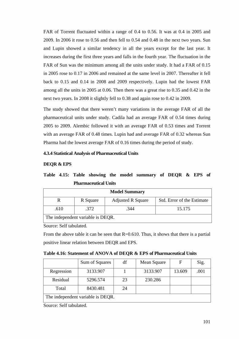
4.3.4 Statistical Analysis of Pharmaceutical Units

DEQR & EPS

Table 4.15: Table showing the model summary of DEQR & EPS of

Pharmaceutical Units

Model Summary


.610 .372 .344 15.175



From the above table it can be seen that R=0.610. Thus, it shows that there is a partial

positive linear relation between DEQR and EPS.

Table 4.16: Statement of ANOVA of DEQR & EPS of Pharmaceutical Units


Regression 3133.907 1 3133.907 13.609 .001

Residual 5296.574 23 230.286

Total 8430.481 24



102

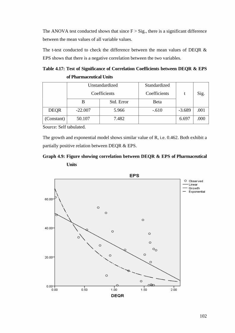
The ANOVA test conducted shows that since F > Sig., there is a significant difference

between the mean values of all variable values.

The t-test conducted to check the difference between the mean values of DEQR &

EPS shows that there is a negative correlation between the two variables.

Table 4.17: Test of Significance of Correlation Coefficients between DEQR & EPS

of Pharmaceutical Units

Unstandardized

Coefficients

Standardized

Coefficients

B Std. Error Beta

t Sig.

DEQR -22.007 5.966 -.610 -3.689 .001

(Constant) 50.107 7.482 6.697 .000


The growth and exponential model shows similar value of R, i.e. 0.462. Both exhibit a

partially positive relation between DEQR & EPS.

Graph 4.9: Figure showing correlation between DEQR & EPS of Pharmaceutical

Units

103

DEQR & FAR

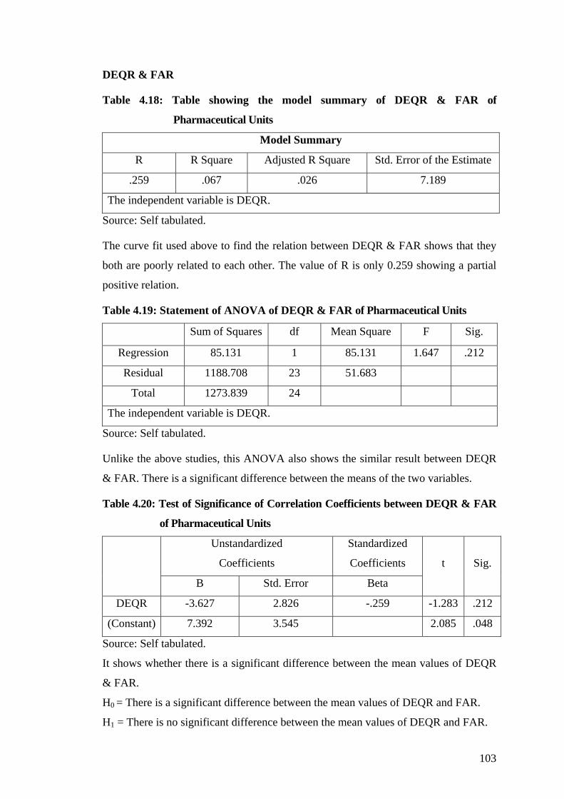
Table 4.18: Table showing the model summary of DEQR & FAR of


Model Summary


.259 .067 .026 7.189



The curve fit used above to find the relation between DEQR & FAR shows that they

both are poorly related to each other. The value of R is only 0.259 showing a partial

positive relation.

Table 4.19: Statement of ANOVA of DEQR & FAR of Pharmaceutical Units


Regression 85.131 1 85.131 1.647 .212

Residual 1188.708 23 51.683

Total 1273.839 24



Unlike the above studies, this ANOVA also shows the similar result between DEQR

& FAR. There is a significant difference between the means of the two variables.

Table 4.20: Test of Significance of Correlation Coefficients between DEQR & FAR

of Pharmaceutical Units

Unstandardized

Coefficients

Standardized

Coefficients

B Std. Error Beta

t Sig.

DEQR -3.627 2.826 -.259 -1.283 .212

(Constant) 7.392 3.545 2.085 .048



& FAR.

H0 = There is a significant difference between the mean values of DEQR and FAR.

H1 = There is no significant difference between the mean values of DEQR and FAR.

104


correlation between the two variables. The growth and exponential models shows the

similar partial positive relation.

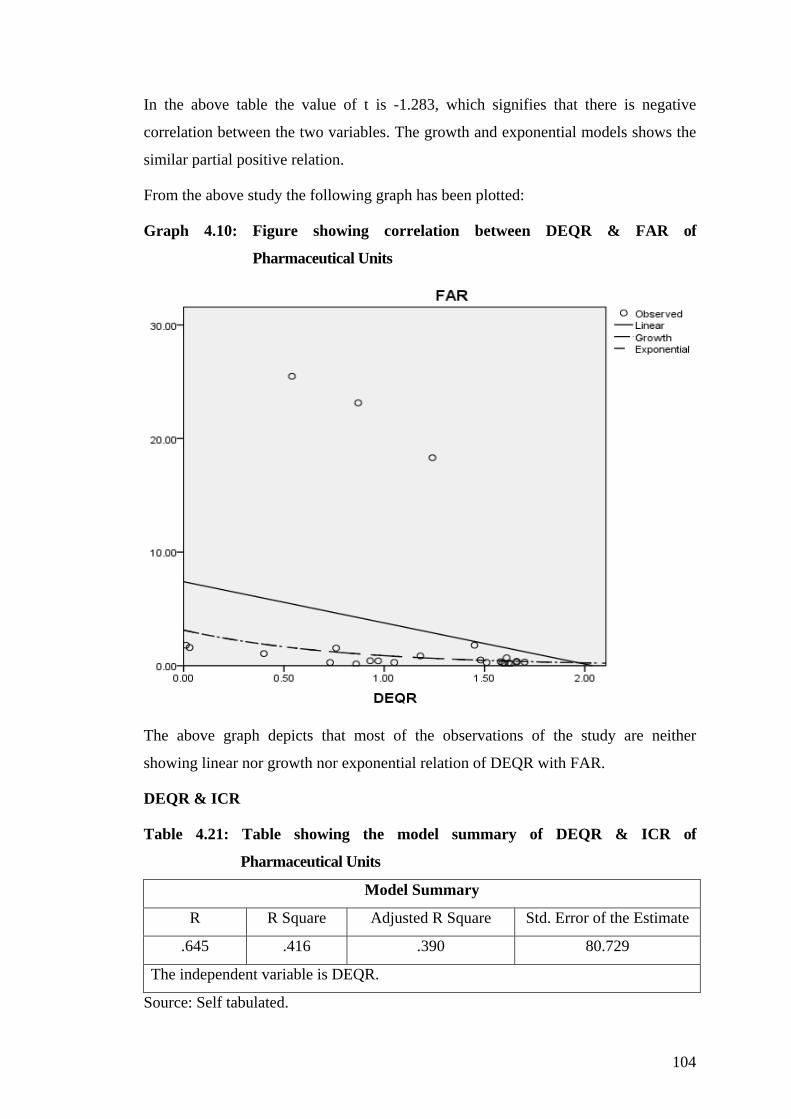
From the above study the following graph has been plotted:

Graph 4.10: Figure showing correlation between DEQR & FAR of


The above graph depicts that most of the observations of the study are neither

showing linear nor growth nor exponential relation of DEQR with FAR.

DEQR & ICR

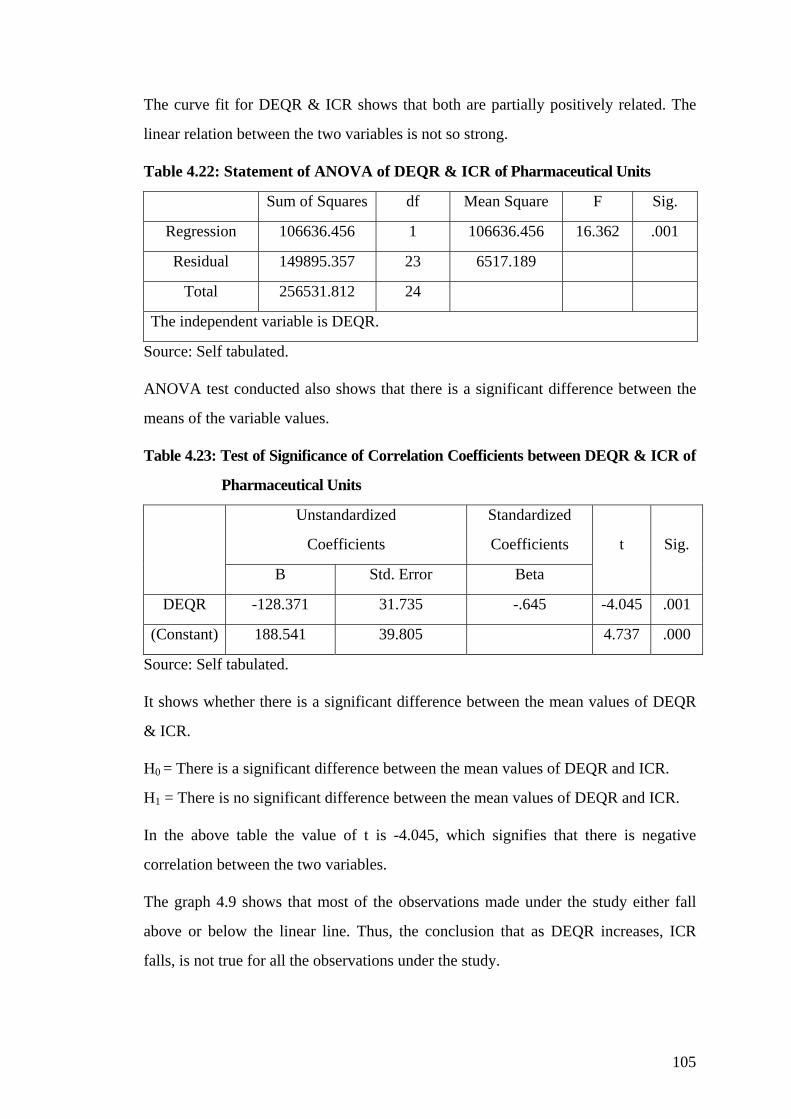
Table 4.21: Table showing the model summary of DEQR & ICR of


Model Summary


.645 .416 .390 80.729



105

The curve fit for DEQR & ICR shows that both are partially positively related. The

linear relation between the two variables is not so strong.

Table 4.22: Statement of ANOVA of DEQR & ICR of Pharmaceutical Units


Regression 106636.456 1 106636.456 16.362 .001

Residual 149895.357 23 6517.189

Total 256531.812 24



ANOVA test conducted also shows that there is a significant difference between the

means of the variable values.

Table 4.23: Test of Significance of Correlation Coefficients between DEQR & ICR of


Unstandardized

Coefficients

Standardized

Coefficients

B Std. Error Beta

t Sig.

DEQR -128.371 31.735 -.645 -4.045 .001

(Constant) 188.541 39.805 4.737 .000



& ICR.

H0 = There is a significant difference between the mean values of DEQR and ICR.

H1 = There is no significant difference between the mean values of DEQR and ICR.



The graph 4.9 shows that most of the observations made under the study either fall

above or below the linear line. Thus, the conclusion that as DEQR increases, ICR

falls, is not true for all the observations under the study.

106

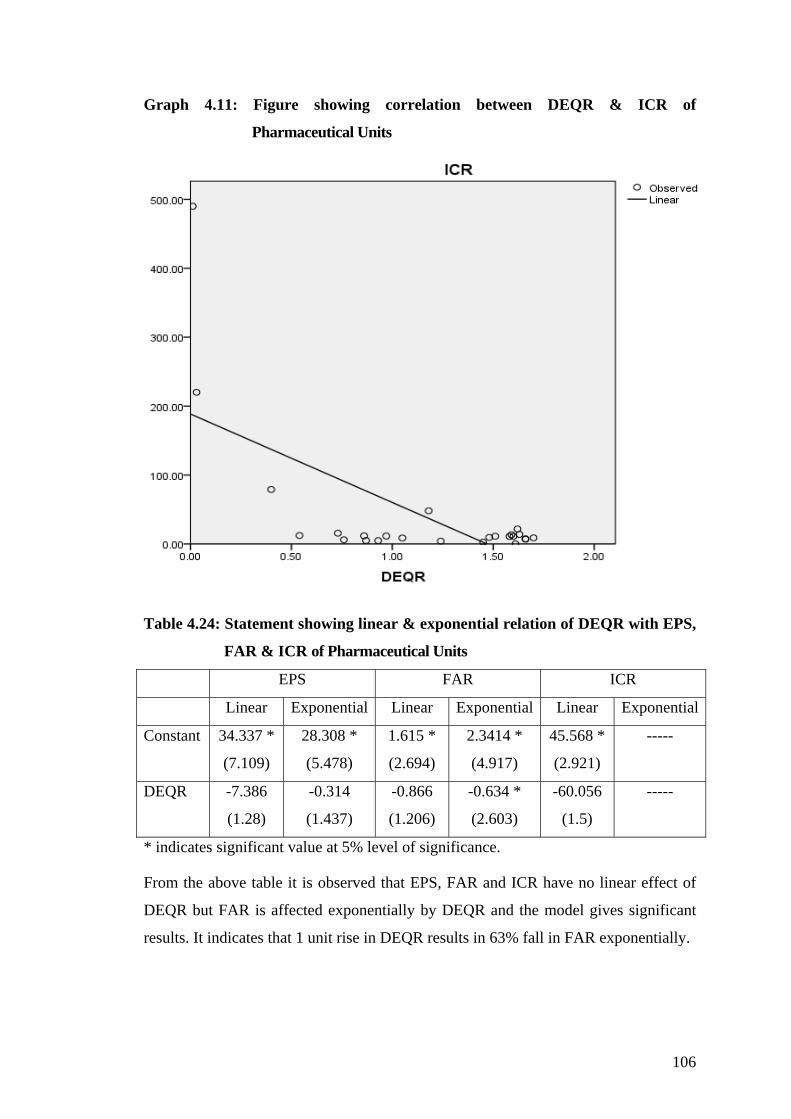
Graph 4.11: Figure showing correlation between DEQR & ICR of


Table 4.24: Statement showing linear & exponential relation of DEQR with EPS,

FAR & ICR of Pharmaceutical Units

EPS FAR ICR

Linear Exponential Linear Exponential Linear Exponential

Constant 34.337 *

(7.109)

28.308 *

(5.478)

1.615 *

(2.694)

2.3414 *

(4.917)

45.568 *

(2.921)

-----

DEQR -7.386

(1.28)

-0.314

(1.437)

-0.866

(1.206)

-0.634 *

(2.603)

-60.056

(1.5)

-----

* indicates significant value at 5% level of significance.

From the above table it is observed that EPS, FAR and ICR have no linear effect of

DEQR but FAR is affected exponentially by DEQR and the model gives significant

results. It indicates that 1 unit rise in DEQR results in 63% fall in FAR exponentially.

107

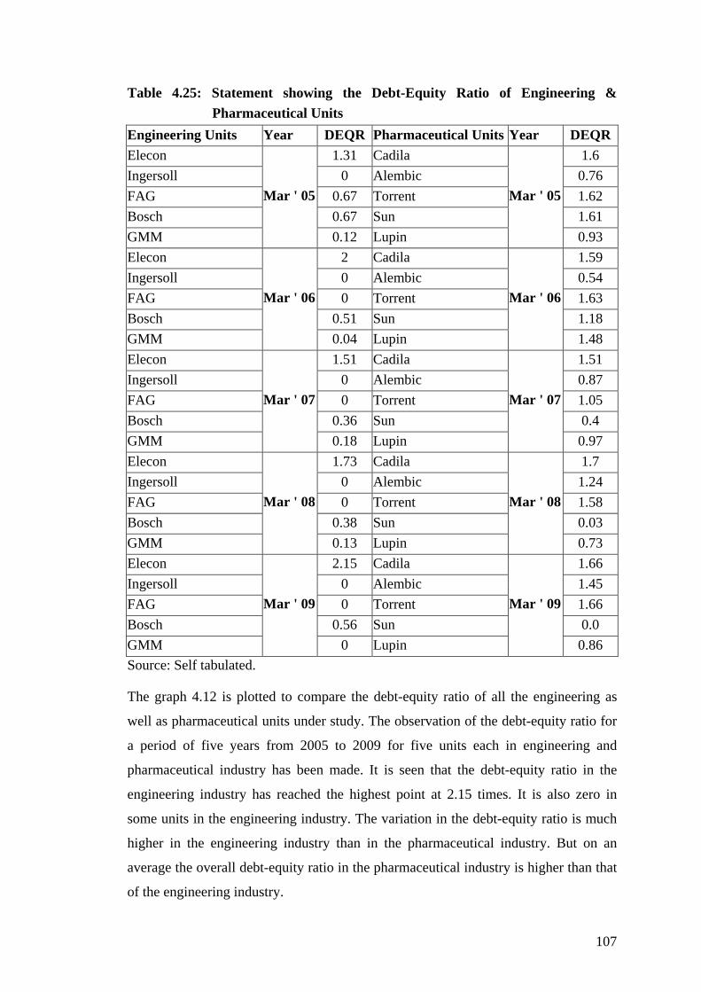
Table 4.25: Statement showing the Debt-Equity Ratio of Engineering & Pharmaceutical Units

Engineering Units Year DEQR Pharmaceutical Units Year DEQRElecon 1.31 Cadila 1.6 Ingersoll 0 Alembic 0.76 FAG 0.67 Torrent 1.62 Bosch 0.67 Sun 1.61 GMM

Mar ' 05

0.12 Lupin

Mar ' 05

0.93 Elecon 2 Cadila 1.59 Ingersoll 0 Alembic 0.54 FAG 0 Torrent 1.63 Bosch 0.51 Sun 1.18 GMM

Mar ' 06

0.04 Lupin

Mar ' 06

1.48 Elecon 1.51 Cadila 1.51 Ingersoll 0 Alembic 0.87 FAG 0 Torrent 1.05 Bosch 0.36 Sun 0.4 GMM

Mar ' 07

0.18 Lupin

Mar ' 07


Mar ' 08

0.13 Lupin

Mar ' 08


Mar ' 09

0 Lupin

Mar ' 09

0.86 Source: Self tabulated.

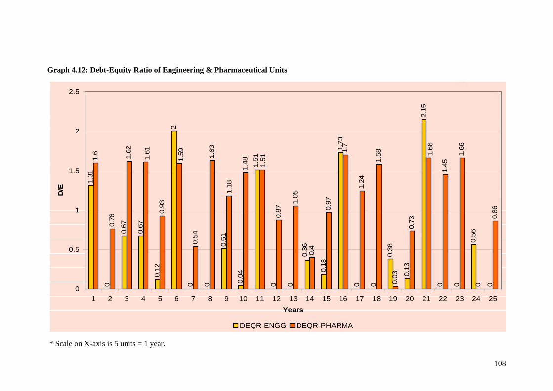
The graph 4.12 is plotted to compare the debt-equity ratio of all the engineering as

well as pharmaceutical units under study. The observation of the debt-equity ratio for

a period of five years from 2005 to 2009 for five units each in engineering and

pharmaceutical industry has been made. It is seen that the debt-equity ratio in the

engineering industry has reached the highest point at 2.15 times. It is also zero in

some units in the engineering industry. The variation in the debt-equity ratio is much

higher in the engineering industry than in the pharmaceutical industry. But on an

average the overall debt-equity ratio in the pharmaceutical industry is higher than that

of the engineering industry.

108

Graph 4.12: Debt-Equity Ratio of Engineering & Pharmaceutical Units

1.31

0

0.67

0.67

0.12

2

0 0

0.51

0.04

0 0

0.18

1.73

0 0

0.38

0.13

2.15

0 0

0.56

0

1.6

0.76

1.62

0.93

0.54

1.63

1.48

0.87

1.05

0.4

0.97

1.7

1.24

1.58

0.03

0.73

1.45

1.66

0

0.86

1.51

0.36

1.66

1.591.61

1.18

1.51

0

0.5

1

1.5

2

2.5

1 2 3 4 5 6 7 8 9 10 11 12 13 14 15 16 17 18 19 20 21 22 23 24 25

Years

D/E

DEQR-ENGG DEQR-PHARMA

* Scale on X-axis is 5 units = 1 year.

109

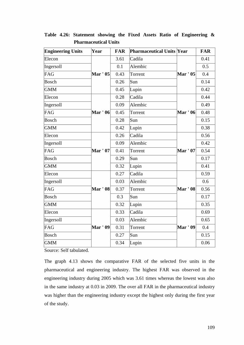
Table 4.26: Statement showing the Fixed Assets Ratio of Engineering & Pharmaceutical Units

Engineering Units Year FAR Pharmaceutical Units Year FAR Elecon 3.61 Cadila 0.41 Ingersoll 0.1 Alembic 0.5 FAG 0.43 Torrent 0.4 Bosch 0.26 Sun 0.14 GMM

Mar ' 05

0.45 Lupin

Mar ' 05

0.42 Elecon 0.28 Cadila 0.44 Ingersoll 0.09 Alembic 0.49 FAG 0.45 Torrent 0.48 Bosch 0.28 Sun 0.15 GMM

Mar ' 06

0.42 Lupin

Mar ' 06


Mar ' 07

0.32 Lupin

Mar ' 07


Mar ' 08

0.32 Lupin

Mar ' 08


Mar ' 09

0.34 Lupin

Mar ' 09


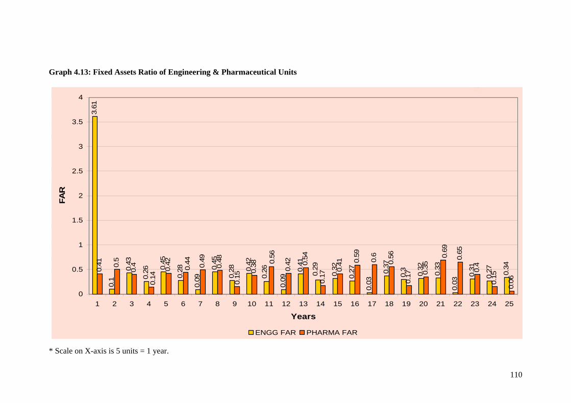
The graph 4.13 shows the comparative FAR of the selected five units in the

pharmaceutical and engineering industry. The highest FAR was observed in the

engineering industry during 2005 which was 3.61 times whereas the lowest was also

in the same industry at 0.03 in 2009. The over all FAR in the pharmaceutical industry

was higher than the engineering industry except the highest only during the first year

of the study.

110

Graph 4.13: Fixed Assets Ratio of Engineering & Pharmaceutical Units

3.61

0.1

0.43

0.26 0.

45

0.28

0.09

0.45

0.28 0.

42

0.09

0.41

0.32

0.27

0.03

0.37

0.3

0.32

0.33

0.03

0.31

0.27 0.340.41 0.

5

0.4

0.42 0.49

0.48

0.38 0.42 0.

54

0.17

0.41 0.

59

0.6

0.56

0.17 0.

35

0.65

0.4

0.15

0.06

0.29

0.26

0.56

0.15

0.14

0.44

0.69

0

0.5

1

1.5

2

2.5

3

3.5

4

1 2 3 4 5 6 7 8 9 10 11 12 13 14 15 16 17 18 19 20 21 22 23 24 25

Years

FAR

ENGG FAR PHARMA FAR


111

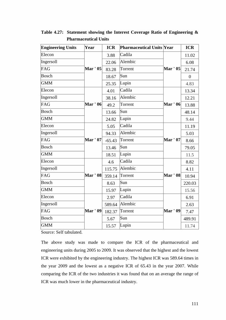
Table 4.27: Statement showing the Interest Coverage Ratio of Engineering & Pharmaceutical Units

Engineering Units Year ICR Pharmaceutical Units Year ICR Elecon 3.88 Cadila 11.02 Ingersoll 22.06 Alembic 6.08 FAG 83.28 Torrent 21.74 Bosch 18.67 Sun 0 GMM

Mar ' 05

25.35 Lupin

Mar ' 05


Mar ' 06

24.82 Lupin

Mar ' 06

9.44 Elecon 5.05 Cadila 11.19 Ingersoll 94.33 Alembic 5.03 FAG -65.43 Torrent 8.66 Bosch 13.46 Sun 79.05 GMM

Mar ' 07

18.51 Lupin

Mar ' 07


Mar ' 08

15.97 Lupin

Mar ' 08


Mar ' 09

15.57 Lupin

Mar ' 09


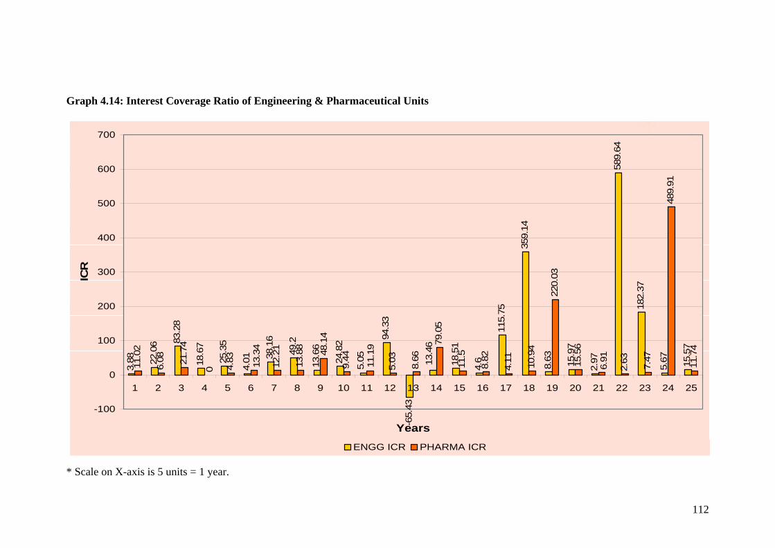
The above study was made to compare the ICR of the pharmaceutical and

engineering units during 2005 to 2009. It was observed that the highest and the lowest

ICR were exhibited by the engineering industry. The highest ICR was 589.64 times in

the year 2009 and the lowest as a negative ICR of 65.43 in the year 2007. While

comparing the ICR of the two industries it was found that on an average the range of

ICR was much lower in the pharmaceutical industry.

112

Graph 4.14: Interest Coverage Ratio of Engineering & Pharmaceutical Units

3.88 22

.06 83

.28

18.6

7

25.3

5

4.01 38

.16

49.2

13.6

6

24.8

2

94.3

3

-65.

43

18.5

1

4.6

115.

75

359.

14

8.63 15.9

7

2.97

589.

64

182.

37

5.67 15

.57

11.0

2

6.08 21

.74

4.83 12.2

1

13.8

8

9.44

5.03

8.66

79.0

5

11.5

8.82

4.11 10.9

4

220.

03

15.5

6

2.63 7.47

489.

91

11.7

4

13.4

6

5.05 11.1

948.1

4

0 13.3

4

6.91

-100

0

100

200

300

400

500

600

700

1 2 3 4 5 6 7 8 9 10 11 12 13 14 15 16 17 18 19 20 21 22 23 24 25

Years

ICR

ENGG ICR PHARMA ICR


113

REFERENCES:

1. Ravi M. Kishore (2004) ‘Financial Management’, Taxmann Allied Services Pvt.

Ltd., pp. 454.

2. Pandey. I. M. (2005), ‘Financial Management’, Vikas Publishing House Pvt.

Ltd., pp. 522+524.

3. Dr. S. N. Maheshwari (2005), ‘Management Accounting And Financial

Control’, Sultan Chand & Sons, New Delhi, pp. B.46.

4. Annual reports of selected pharmaceutical and engineering companies from

2005-06 to 2009-10.

WEBSITES

1. www.google.com

2. www.gujaratonline.in

3. www.investopedia.com

4. www.moneycontrol.com

Documents

CHAPTER - IV ANALYSIS OF CAPITAL STRUCTURE OF SELECTED UNITS