62

CHAPTER IV

SEDIMENTOLOGY

4.1 INTRODUCTION

Sediment texture refers to the shape, size and three dimensional

arrangements of the particles that make up sediment or a sedimentary rock. Particle

size distribution in a clastic sedimentary rock is sensitive to the physical changes of

the transporting media and the depositional basin. Systematic presentation and

analysis of grain size data provide basis for the reconstruction of sedimentary

processes including identification of depositional environment.

Since nineties sedimentologists are using grain size data for the

interpretation of sedimentary processes. An earliest effort for the systematic

analysis of grain size data was made by Udden (1898, 1914), Wentworth (1922).

Oseen (1913) and Rubey (1933) developed equations to extend the limit of settling

velocity techniques to measure the size of coarse silt. Trask (1932), Krumbein

(1934), Krumbein and Pettijohn (1938), Otto (1939), Twenhofel and Tyler (1941),

Inman (1952), Spencer (1952) and others advocated the application of statistical

techniques to characterize the frequency distribution of clastic sediments.

Application of granulometric analysis in hydrodynamics and environmental

interpretation was empahasised by Hjulstorm (1939), Doeglas (1946), Inman

(1949), Bagnold (1946, 1956), Passega (1957, 1964), Folk and Ward (1957),

Mason and Folk (1958), Harris (1958a), Roser and Head (1961), Moss (1963),

Sahu (1964), Krinsely and Funnell (1965), Klovan (1966), Friedman (1967),

Koldijk (1968), Chappell (1967), Moiola and Weiser (1968), Hails and Hoyt

63

(1969), Visher (1969), Buller and Mc Manus (1972), Qidwai and Cassyap (1978),

Swan et al., (1978); and others. Recent works by different researchers, viz.

Mahender (1996), Joshep et al., (1997), Hanamgond and Chavadi (1998),

Majumdar and Ganapati (1998), Murkute (2001a, 2001b), Raman and Reddy

(2001), Bhat et al., (2002), Rao et al., (2008), Ashok and Rupesh (2009a, 2009b),

Ashok and Neloy Khare (2009), Omali et al., (2011), Odedede et al., (2013),

Gideon et al., (2014) and Devi et al., (2014) and others amply testify the

significance of the grain size study.

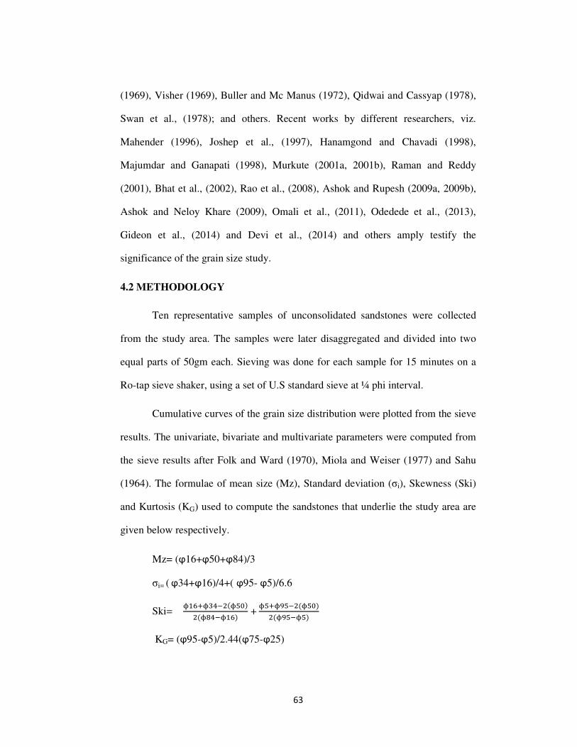
4.2 METHODOLOGY

Ten representative samples of unconsolidated sandstones were collected

from the study area. The samples were later disaggregated and divided into two

equal parts of 50gm each. Sieving was done for each sample for 15 minutes on a

Ro-tap sieve shaker, using a set of U.S standard sieve at ¼ phi interval.

Cumulative curves of the grain size distribution were plotted from the sieve

results. The univariate, bivariate and multivariate parameters were computed from

the sieve results after Folk and Ward (1970), Miola and Weiser (1977) and Sahu

(1964). The formulae of mean size (Mz), Standard deviation (σi), Skewness (Ski)

and Kurtosis (KG) used to compute the sandstones that underlie the study area are

given below respectively.

Mz= (ϕ16+ϕ50+ϕ84)/3

σi= ( ϕ34+ϕ16)/4+( ϕ95- ϕ5)/6.6

Ski= ������������

�� ������ +

���������

������

KG= (ϕ95-ϕ5)/2.44(ϕ75-ϕ25)

64

4.3 TEXTURAL CHARACTERISTICS

4.3.1 Mean

Mean represents the average size of the total distribution of sediments. It

serves as an index to measure the nature as well as the depositional environment

of the sediments. It is the function of total amount of sediments available, the

amount of energy imported to the sediments and nature of the transporting agent.

The energy of transporting agent includes the degree of turbulence and the role

played by currents and waves.

The mean size of the study area sandstones ranges from 0.038 φ to 1.67 φ

indicating medium to coarse grained. Seralathan (1979) has noted that the

increase in mean size to coarse sand around Pondicherry is generally attributed to

the removal of fine fraction in high energy condition.

4.3.2 Standard Deviation

Standard deviation is a measure of uniformity or sorting. It is also the

resultant character of sediments controlled by size, shape and specific gravity of

sediments and energy and time involved in transporting fine. It is noted that the

standard deviation decreases towards the sample of lower mean size. In other

words, the sorting improves with the lowering of mean size. As a result, the

sediments having fine sand (between 2.25 φ and 4.25 φ) exhibit well sorted

nature. This phenomenon has also been noted by Inman (1952), Friedman (1967)

and Krumbein (1984).

65

Pheleger (1969) has noted that poorly sorted nature of sediments in the

paleo-barriers along the Mexican coast. Zenkovitch (1969) and Reineck and

Singh (1986) have also reported the occurrence of poorly sorted sediments and

admixture of pebbles in the barriers occurring in front of the coastal lagoons. The

presence of minor amount of pebbles in this site may also be accounted for such

admixture.

In the study area, the standard deviation value for sandstone ranges from

0.28 φ to 1.67 φ indicating very well sorted to poorly sorted nature. The well

sorted to poor sorting nature indicates in a place where there is a continuous, slow

deposition of sediments. The skewness values on the other hand range from 0.564

to 0.766 and indicate dominantly fine skewed nature of sediments. The studied

samples show kurtosis values ranging from 0.195 to 0.946 and the samples are

distinctly very platykurtic.

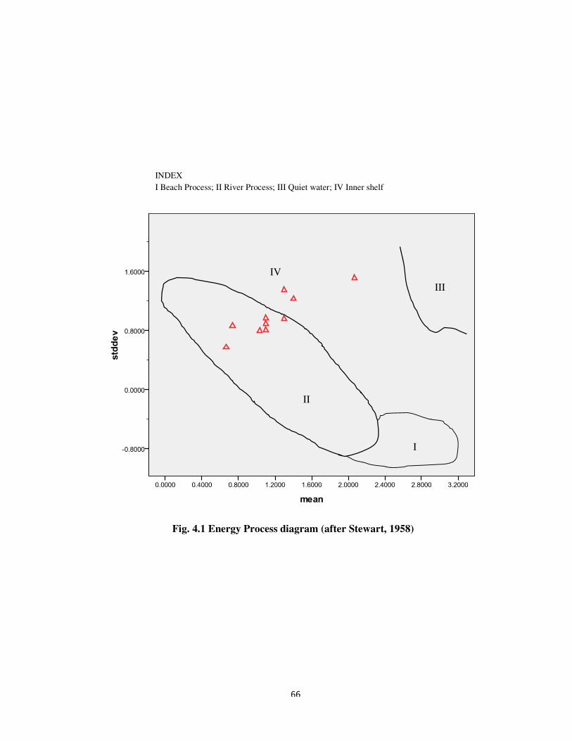
4.3.3 Mean VS Standard Deviation

The scatter plot between mean size and standard deviation (Fig. 4.1)

shows the samples falls in the river process field. Its indicates fluvial signature in

the sediments and therefore the depositional environment is dominantly a fluvial

system.

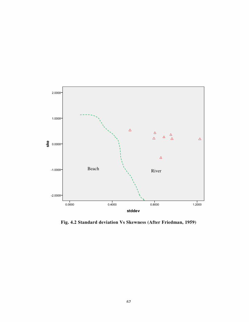
4.3.4 Standard Deviation Versus Skewness

The scatter plot constructed using the standard deviation and skewness of

the study area samples (Fig. 4.2) reveals to confirm the sediments depositional

environment is fluvial system.

66

Fig. 4.1 Energy Process diagram (after Stewart, 1958)

I

II

III

IV

INDEX

I Beach Process; II River Process; III Quiet water; IV Inner shelf

67

Fig. 4.2 Standard deviation Vs Skewness (After Friedman, 1959)

Beach River

68

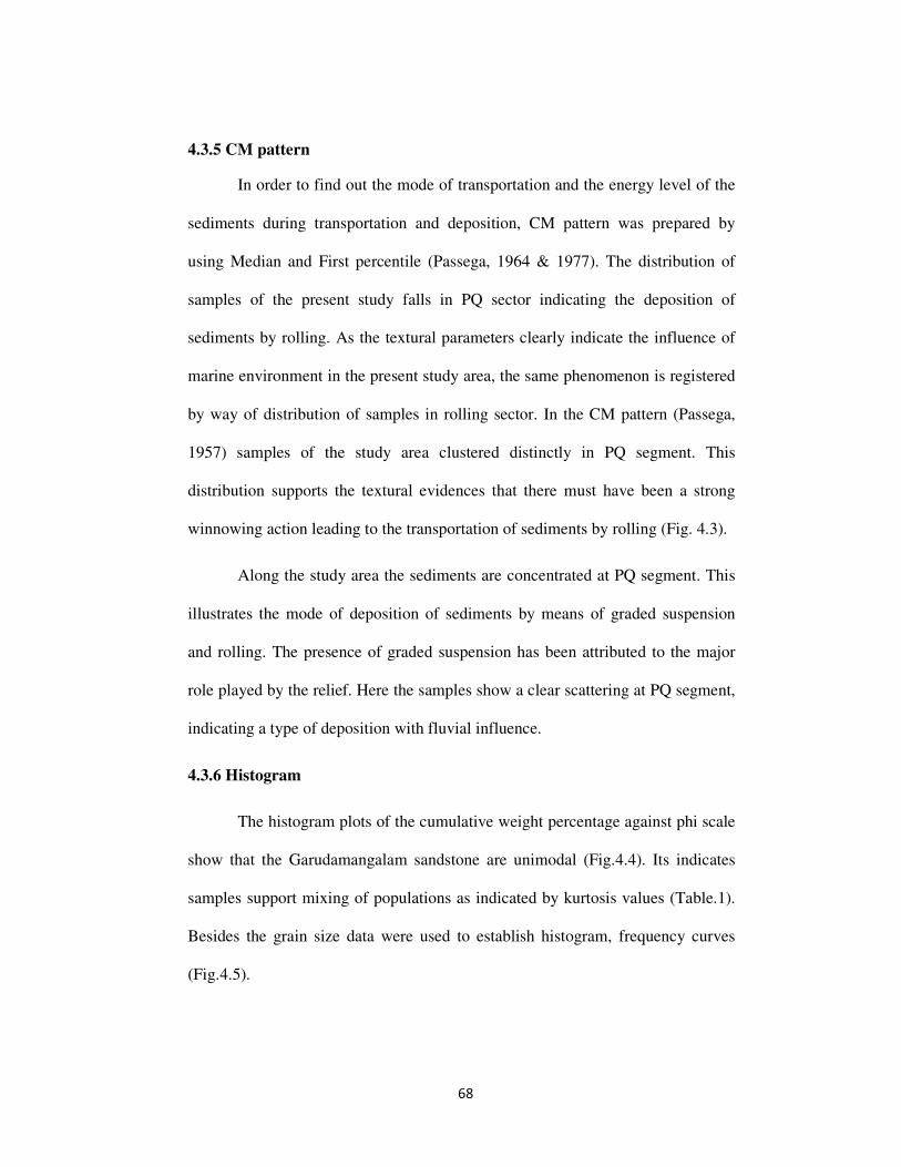
4.3.5 CM pattern

In order to find out the mode of transportation and the energy level of the

sediments during transportation and deposition, CM pattern was prepared by

using Median and First percentile (Passega, 1964 & 1977). The distribution of

samples of the present study falls in PQ sector indicating the deposition of

sediments by rolling. As the textural parameters clearly indicate the influence of

marine environment in the present study area, the same phenomenon is registered

by way of distribution of samples in rolling sector. In the CM pattern (Passega,

1957) samples of the study area clustered distinctly in PQ segment. This

distribution supports the textural evidences that there must have been a strong

winnowing action leading to the transportation of sediments by rolling (Fig. 4.3).

Along the study area the sediments are concentrated at PQ segment. This

illustrates the mode of deposition of sediments by means of graded suspension

and rolling. The presence of graded suspension has been attributed to the major

role played by the relief. Here the samples show a clear scattering at PQ segment,

indicating a type of deposition with fluvial influence.

4.3.6 Histogram

The histogram plots of the cumulative weight percentage against phi scale

show that the Garudamangalam sandstone are unimodal (Fig.4.4). Its indicates

samples support mixing of populations as indicated by kurtosis values (Table.1).

Besides the grain size data were used to establish histogram, frequency curves

(Fig.4.5).

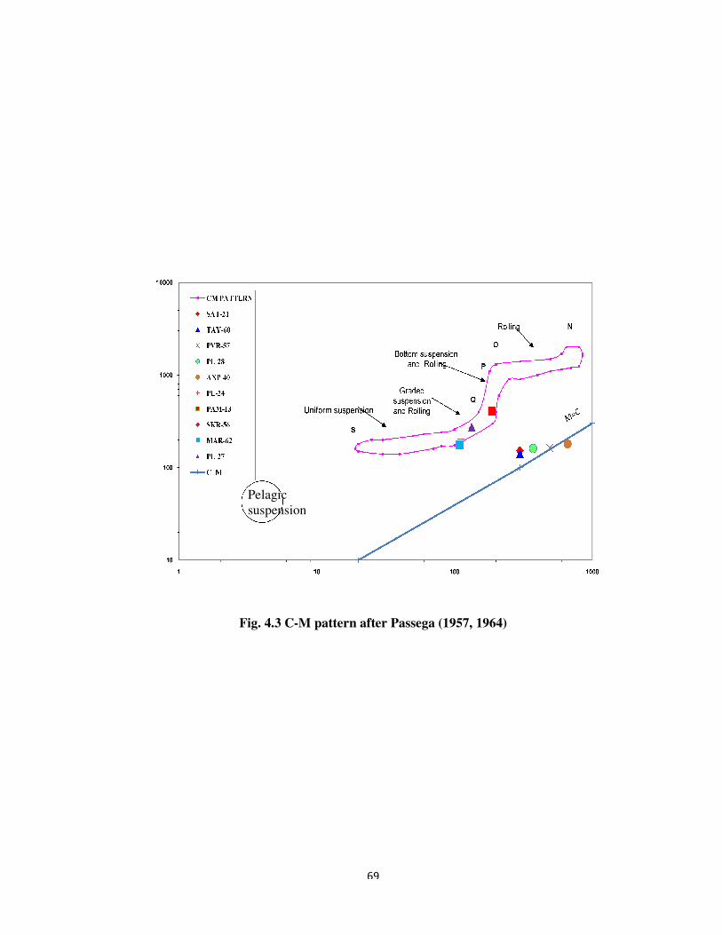
Fig. 4.3 C

Pelagic

suspension

69

4.3 C-M pattern after Passega (1957, 1964)

Pelagic

suspension

70

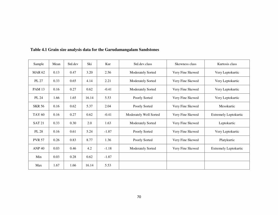
Table 4.1 Grain size analysis data for the Garudamangalam Sandstones

Sample Mean Std.dev Ski Kur Std.dev.class Skewness class Kurtosis class

MAR 62 0.13 0.47 3.20 2.56 Moderately Sorted Very Fine Skewed Very Leptokurtic

PL 27 0.33 0.65 4.14 2.21 Moderately Sorted Very Fine Skewed Very Leptokurtic

PAM 13 0.16 0.27 0.62 -0.41 Moderately Sorted Very Fine Skewed Very Leptokurtic

PL 24 1.66 1.65 16.14 5.53 Poorly Sorted Very Fine Skewed Very Leptokurtic

SKR 56 0.16 0.62 5.37 2.04 Poorly Sorted Very Fine Skewed Mesokurtic

TAY 60 0.16 0.27 0.62 -0.41 Moderately Well Sorted Very Fine Skewed Extremely Leptokurtic

SAT 21 0.33 0.30 2.0 1.63 Moderately Sorted Very Fine Skewed Leptokurtic

PL 28 0.16 0.61 5.24 -1.87 Poorly Sorted Very Fine Skewed Very Leptokurtic

PVR 57 0.26 0.83 8.77 1.36 Poorly Sorted Very Fine Skewed Platykurtic

ANP 40 0.03 0.46 4.2 -1.18 Moderately Sorted Very Fine Skewed Extremely Leptokurtic

Min 0.03 0.28 0.62 -1.87

Max 1.67 1.66 16.14 5.53

71

Fig. 4.4 Histogram plots of the Garudamangalam Sandstone

72

4.4 Histogram plots of the Garudamangalam Sandstone

Fig. 4.5 Cumulative frequency curves of Garudamangalam sandstones

73

4.5 Cumulative frequency curves of Garudamangalam sandstones4.5 Cumulative frequency curves of Garudamangalam sandstones