Embed Size (px)
DESCRIPTION
Understanding how to compute analysis using Markov
Citation preview

Markov Analysis
Chapter 16
To accompanyQuantitative Analysis for Management, Tenth Edition, by Render, Stair, and Hanna Power Point slides created by Jeff Heyl © 2009 Prentice-Hall, Inc.
Learning Objectives
1. Determine future states or conditions by using Markov analysis
2. Compute long-term or steady-state conditions by using only the matrix of transition probabilities
3. Understand the use of absorbing state analysis in predicting future conditions
After completing this chapter, students will be able to:After completing this chapter, students will be able to:
Chapter Outline
16.116.1 Introduction16.216.2 States and State Probabilities16.316.3 Matrix of Transition Probabilities16.416.4 Predicting Future Market Share16.516.5 Markov Analysis of Machine Operations16.616.6 Equilibrium Conditions16.716.7 Absorbing States and the Fundamental
Matrix: Accounts Receivable Application
Introduction
Markov analysisMarkov analysis is a technique that deals with the probabilities of future occurrences by analyzing presently known probabilities
It has numerous applications in business Markov analysis makes the assumption that
the system starts in an initial state or condition
The probabilities of changing from one state to another are called a matrix of transition probabilities
Solving Markov problems requires basic matrix manipulation
Introduction
This discussion will be limited to Markov problems that follow four assumptions
1. There are a limited or finite number of possible states
2. The probability of changing states remains the same over time
3. We can predict any future state from the previous state and the matrix of transition probabilities
4. The size and makeup of the system do not change during the analysis
States and State Probabilities
States are used to identify all possible conditions of a process or system
It is possible to identify specific states for many processes or systems
In Markov analysis we assume that the states are both collectively exhaustivecollectively exhaustive and mutually mutually exclusiveexclusive
After the states have been identified, the next step is to determine the probability that the system is in this state
States and State Probabilities
The information is placed into a vector of state probabilities
(i) = vector of state probabilities for period i
= (1, 2, 3, … , n)
where
n= number of states
1, 2, … , n= probability of being in state 1, state 2, …, state n
States and State Probabilities
In some cases it is possible to know with complete certainty what state an item is in
Vector states can then be represented as
(1) = (1, 0)
where
(1)= vector of states for the machine in period 1
1 = 1 = probability of being in the first state
2 = 0 = probability of being in the second state
The Vector of State Probabilities for Three Grocery Stores Example
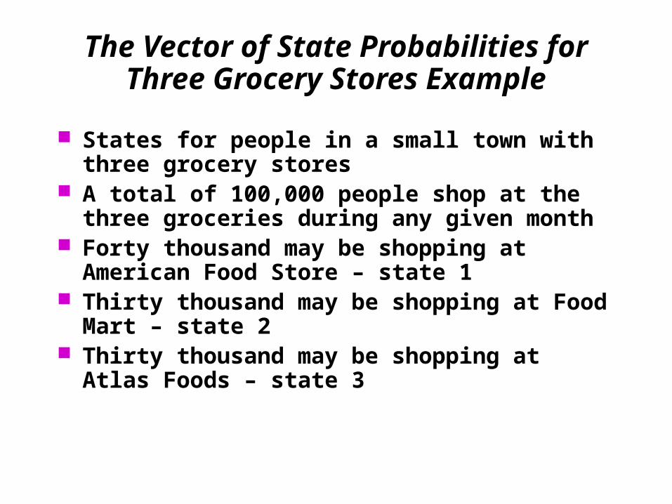
States for people in a small town with three grocery stores
A total of 100,000 people shop at the three groceries during any given month
Forty thousand may be shopping at American Food Store – state 1
Thirty thousand may be shopping at Food Mart – state 2
Thirty thousand may be shopping at Atlas Foods – state 3
The Vector of State Probabilities for Three Grocery Stores Example
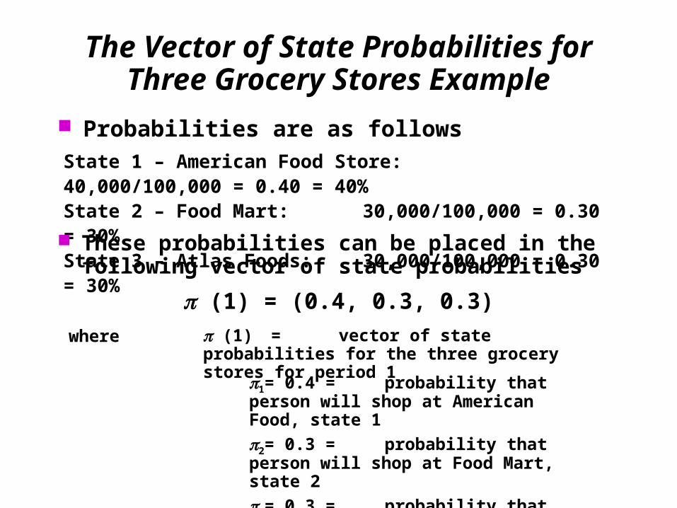
Probabilities are as followsState 1 – American Food Store: 40,000/100,000 = 0.40 = 40%State 2 – Food Mart: 30,000/100,000 = 0.30 = 30%State 3 – Atlas Foods: 30,000/100,000 = 0.30 = 30%
These probabilities can be placed in the following vector of state probabilities
(1) = (0.4, 0.3, 0.3)
where (1)=vector of state probabilities for the three grocery stores for period 1
1= 0.4 = probability that person will shop at American Food, state 1
2= 0.3 = probability that person will shop at Food Mart, state 2
3= 0.3 = probability that person will shop at Atlas Foods, state 3
The Vector of State Probabilities for Three Grocery Stores Example
The probabilities of the vector states represent the market sharesmarket shares for the three groceries
Management will be interested in how their market share changes over time
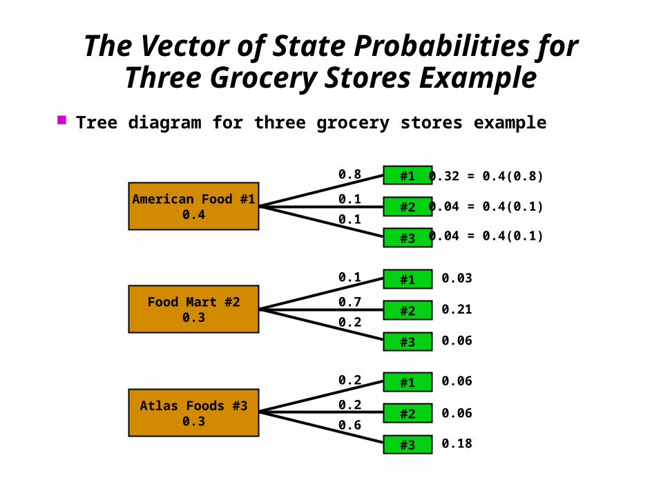
Figure 16.1 shows a tree diagram of how the market shares in the next month
The Vector of State Probabilities for Three Grocery Stores Example
Tree diagram for three grocery stores example
0.8
0.1
0.1
#1
#2
#3
0.32 = 0.4(0.8)
0.04 = 0.4(0.1)
0.04 = 0.4(0.1)
0.1
0.2
0.7#2
#3
#1 0.03
0.21
0.06
0.2
0.6
0.2
#1
#2
#3
0.06
0.06
0.18
American Food #10.4
Food Mart #20.3
Atlas Foods #30.3
Matrix of Transition Probabilities
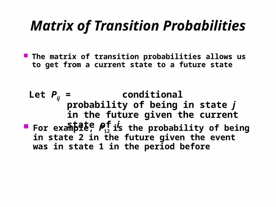
The matrix of transition probabilities allows us to get from a current state to a future state
Let Pij = conditional probability of being in state j in the future given the current state of i
For example, P12 is the probability of being in state 2 in the future given the event was in state 1 in the period before
Matrix of Transition Probabilities
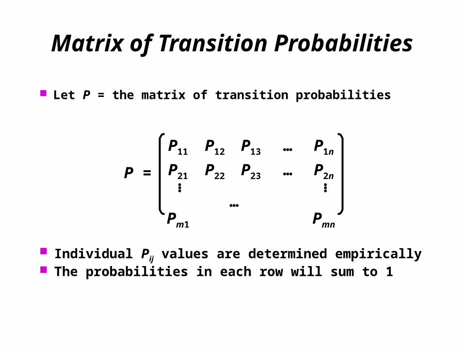
Let P = the matrix of transition probabilities
P =
P11 P12 P13 … P1n
P21 P22 P23 … P2n
Pm1 Pmn
…
… …
Individual Pij values are determined empirically The probabilities in each row will sum to 1
Transition Probabilities for the Three Grocery Stores
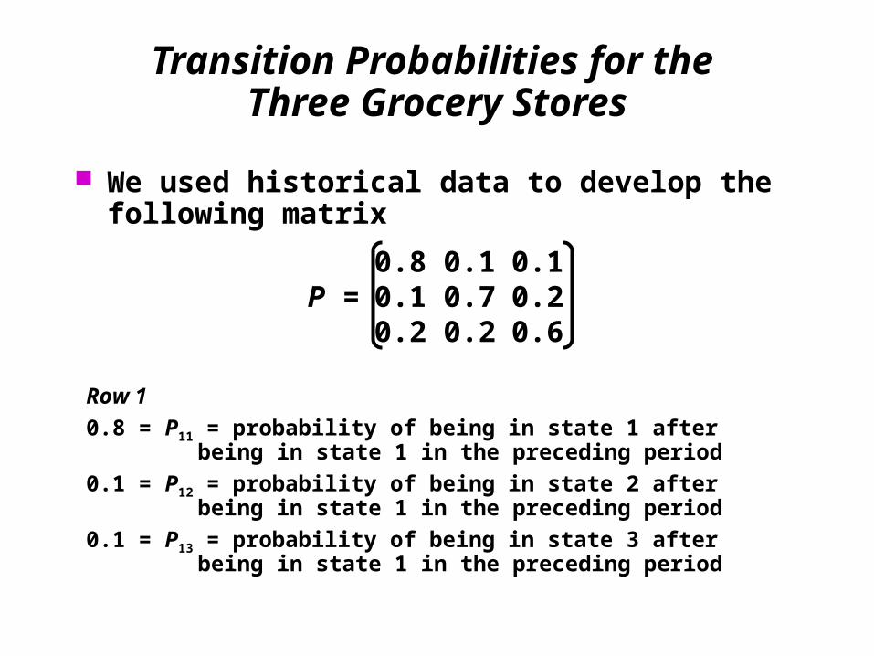
We used historical data to develop the following matrix
P =0.8 0.1 0.10.1 0.7 0.20.2 0.2 0.6
Row 1
0.8 = P11 = probability of being in state 1 after being in state 1 in the preceding period
0.1 = P12 = probability of being in state 2 after being in state 1 in the preceding period
0.1 = P13 = probability of being in state 3 after being in state 1 in the preceding period
Transition Probabilities for the Three Grocery Stores
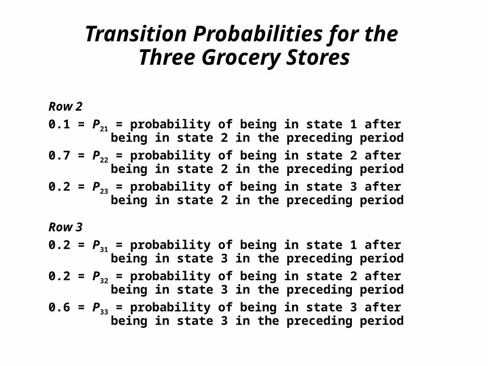
Row 2
0.1 = P21 = probability of being in state 1 after being in state 2 in the preceding period
0.7 = P22 = probability of being in state 2 after being in state 2 in the preceding period
0.2 = P23 = probability of being in state 3 after being in state 2 in the preceding period
Row 3
0.2 = P31 = probability of being in state 1 after being in state 3 in the preceding period
0.2 = P32 = probability of being in state 2 after being in state 3 in the preceding period
0.6 = P33 = probability of being in state 3 after being in state 3 in the preceding period
Predicting Future Market Shares
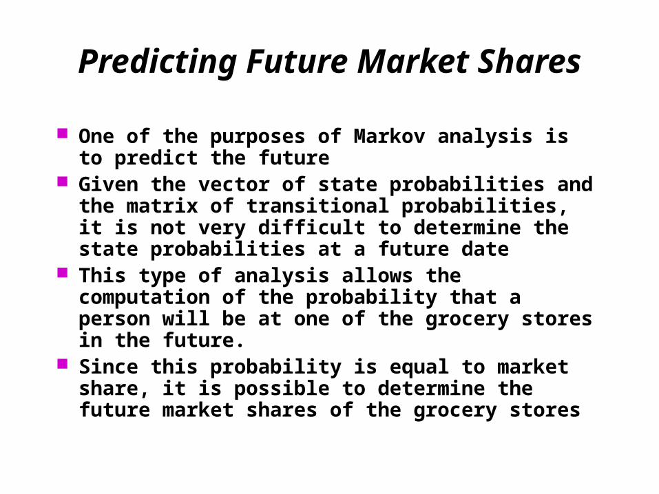
One of the purposes of Markov analysis is to predict the future
Given the vector of state probabilities and the matrix of transitional probabilities, it is not very difficult to determine the state probabilities at a future date
This type of analysis allows the computation of the probability that a person will be at one of the grocery stores in the future.
Since this probability is equal to market share, it is possible to determine the future market shares of the grocery stores
Predicting Future Market Shares
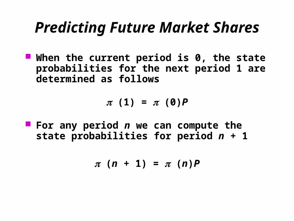
When the current period is 0, the state probabilities for the next period 1 are determined as follows
(1) = (0)P
For any period n we can compute the state probabilities for period n + 1
(n + 1) = (n)P
Predicting Future Market Shares
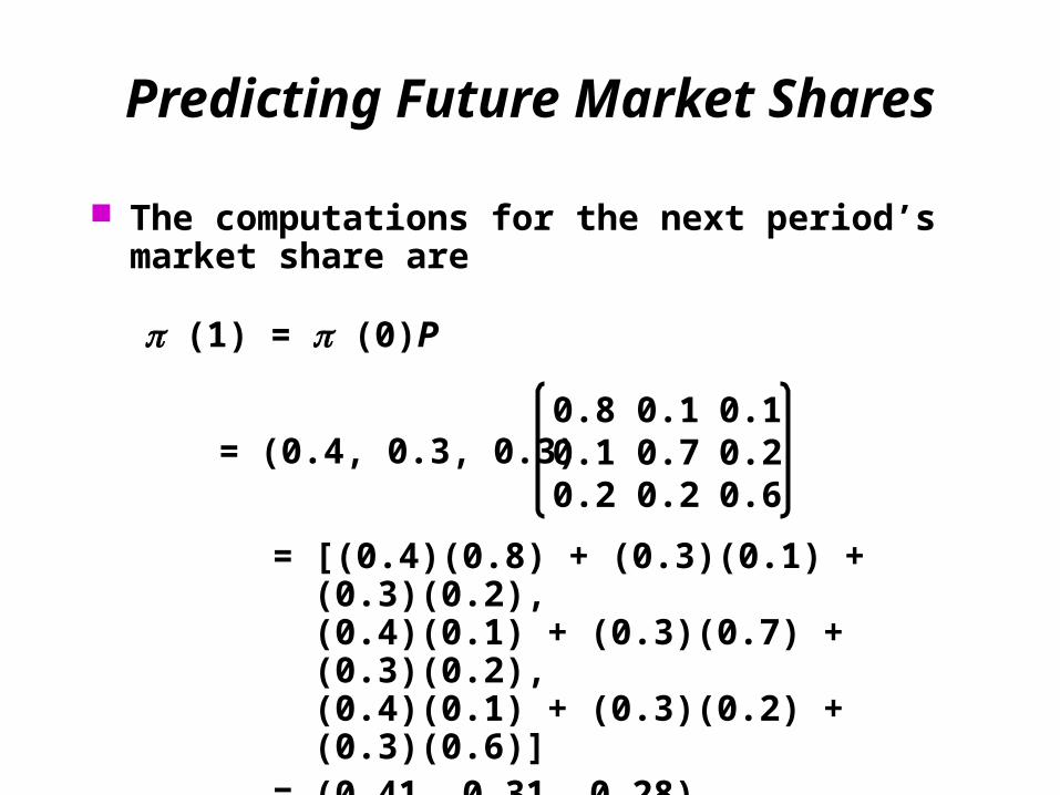
The computations for the next period’s market share are
(1) = (0)P
= (0.4, 0.3, 0.3)0.8 0.1 0.10.1 0.7 0.20.2 0.2 0.6
= [(0.4)(0.8) + (0.3)(0.1) + (0.3)(0.2), (0.4)(0.1) + (0.3)(0.7) + (0.3)(0.2), (0.4)(0.1) + (0.3)(0.2) + (0.3)(0.6)]
= (0.41, 0.31, 0.28)
Predicting Future Market Shares
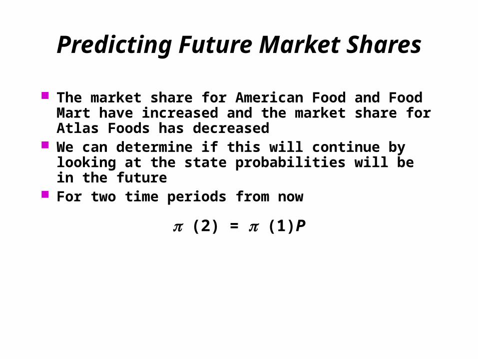
The market share for American Food and Food Mart have increased and the market share for Atlas Foods has decreased
We can determine if this will continue by looking at the state probabilities will be in the future
For two time periods from now
(2) = (1)P
Predicting Future Market Shares
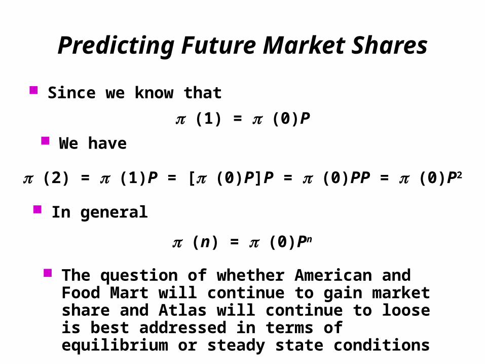
Since we know that
(1) = (0)P
(2) = (1)P = [ (0)P]P = (0)PP = (0)P2
We have
In general
(n) = (0)Pn
The question of whether American and Food Mart will continue to gain market share and Atlas will continue to loose is best addressed in terms of equilibrium or steady state conditions
Markov Analysis of Machine Operations
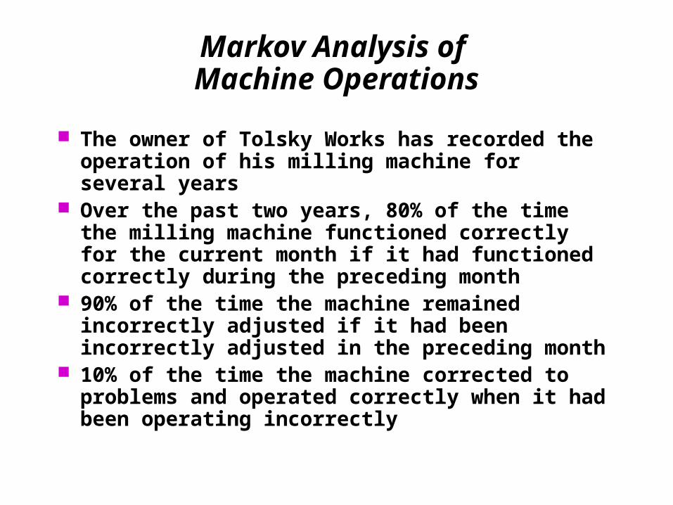
The owner of Tolsky Works has recorded the operation of his milling machine for several years
Over the past two years, 80% of the time the milling machine functioned correctly for the current month if it had functioned correctly during the preceding month
90% of the time the machine remained incorrectly adjusted if it had been incorrectly adjusted in the preceding month
10% of the time the machine corrected to problems and operated correctly when it had been operating incorrectly
Markov Analysis of Machine Operations
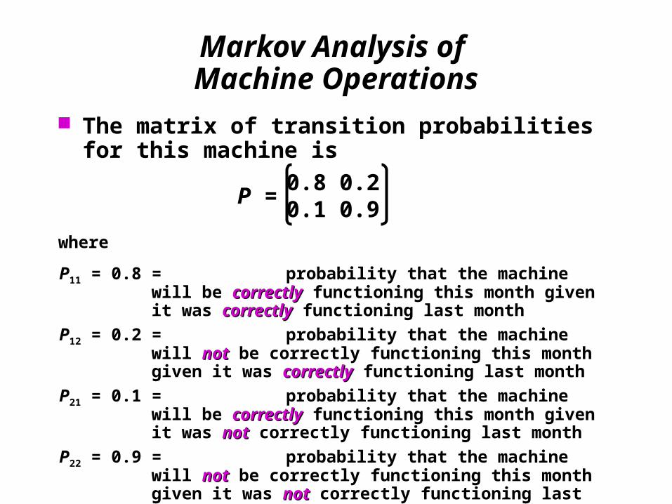
The matrix of transition probabilities for this machine is
0.8 0.20.1 0.9
P =
where
P11 = 0.8 = probability that the machine will be correctlycorrectly functioning this month given it was correctlycorrectly functioning last month
P12 = 0.2 = probability that the machine will notnot be correctly functioning this month given it was correctlycorrectly functioning last month
P21 = 0.1 = probability that the machine will be correctlycorrectly functioning this month given it was notnot correctly functioning last month
P22 = 0.9 = probability that the machine will notnot be correctly functioning this month given it was notnot correctly functioning last month
Markov Analysis of Machine Operations
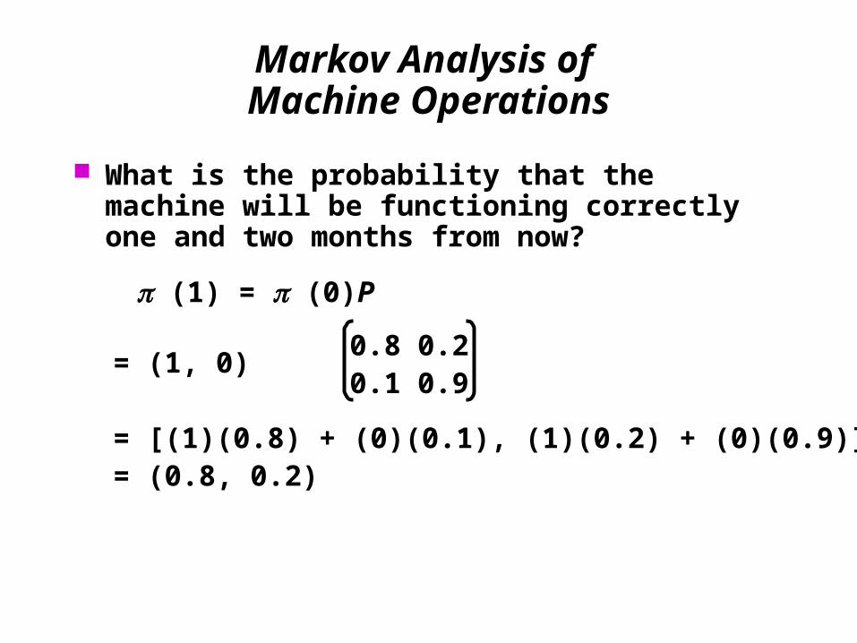
What is the probability that the machine will be functioning correctly one and two months from now?
(1) = (0)P
= (1, 0)
= [(1)(0.8) + (0)(0.1), (1)(0.2) + (0)(0.9)]= (0.8, 0.2)
0.8 0.20.1 0.9
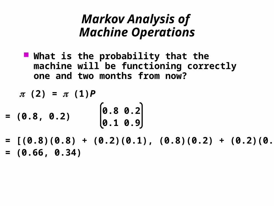
Markov Analysis of Machine Operations
What is the probability that the machine will be functioning correctly one and two months from now?
(2) = (1)P
= (0.8, 0.2)
= [(0.8)(0.8) + (0.2)(0.1), (0.8)(0.2) + (0.2)(0.9)]= (0.66, 0.34)
0.8 0.20.1 0.9
Equilibrium Conditions
It is easy to imagine that all market shares will eventually be 0 or 1
But equilibrium shareequilibrium share of the market values or probabilities generally exist
An equilibrium conditionequilibrium condition exists if state probabilities do not change after a large number of periods
At equilibrium, state probabilities for the next period equal the state probabilities for current period
Equilibrium state probabilities can be computed by repeating Markov analysis for a large number of periods

Equilibrium Conditions
It is always true that
(next period) = (this period)P
(n + 1) = (n) At equilibrium
Or (n + 1) = (n)P
So at equilibrium (n + 1) = (n)P = (n)
Or = P
Equilibrium Conditions
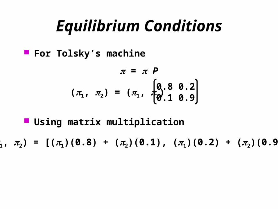
For Tolsky’s machine
= P
(1, 2) = (1, 2)0.8 0.20.1 0.9
Using matrix multiplication
(1, 2) = [(1)(0.8) + (2)(0.1), (1)(0.2) + (2)(0.9)]
Equilibrium Conditions
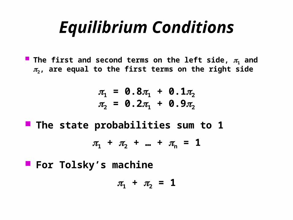
The first and second terms on the left side, 1 and 2, are equal to the first terms on the right side
1 = 0.81 + 0.12
2 = 0.21 + 0.92
The state probabilities sum to 1
1 + 2 + … + n = 1
For Tolsky’s machine
1 + 2 = 1
Equilibrium Conditions
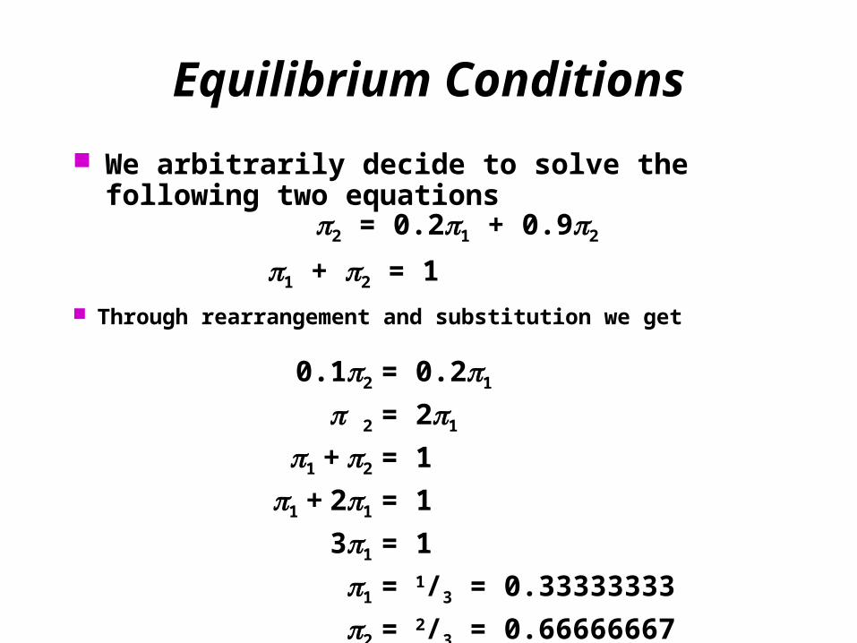
We arbitrarily decide to solve the following two equations
0.12 = 0.21
2 = 21
1 + 2 = 1
1 + 21 = 1
31 = 1
1 = 1/3 = 0.33333333
2 = 2/3 = 0.66666667
Through rearrangement and substitution we get
1 + 2 = 1
2 = 0.21 + 0.92
Absorbing States and the Fundamental Matrix
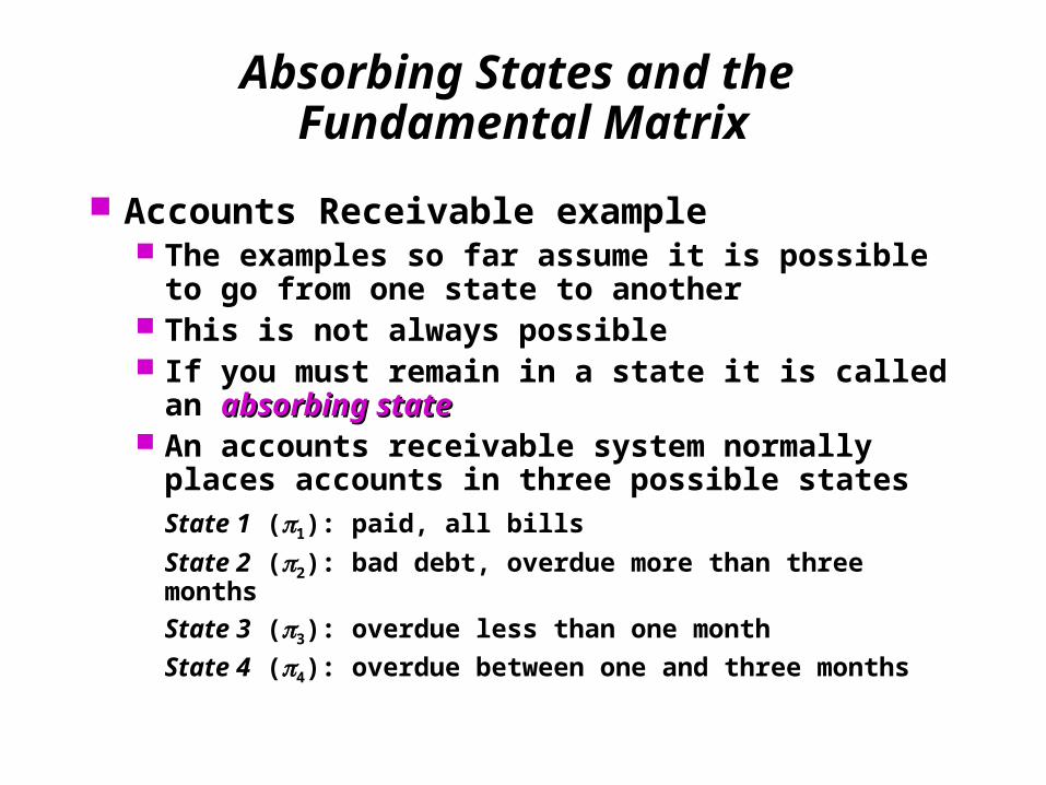
Accounts Receivable example The examples so far assume it is possible to go
from one state to another This is not always possible If you must remain in a state it is called an
absorbing stateabsorbing state An accounts receivable system normally places
accounts in three possible statesState 1 (1): paid, all bills
State 2 (2): bad debt, overdue more than three months
State 3 (3): overdue less than one month
State 4 (4): overdue between one and three months
Absorbing States and the Fundamental Matrix
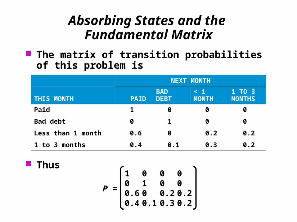
The matrix of transition probabilities of this problem is
NEXT MONTH
THIS MONTH PAIDBAD DEBT
< 1 MONTH
1 TO 3 MONTHS
Paid 1 0 0 0
Bad debt 0 1 0 0
Less than 1 month 0.6 0 0.2 0.2
1 to 3 months 0.4 0.1 0.3 0.2
Thus
P =
1 0 0 00 1 0 00.6 0 0.2 0.20.4 0.1 0.3 0.2
Absorbing States and the Fundamental Matrix
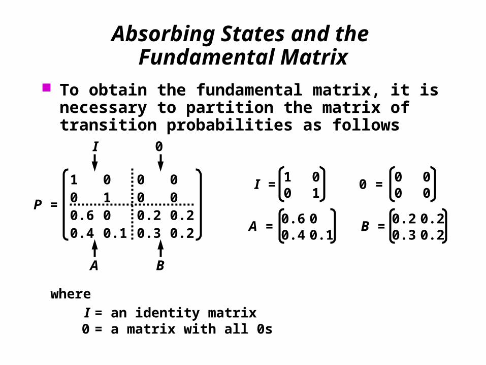
To obtain the fundamental matrix, it is necessary to partition the matrix of transition probabilities as follows
P =
1 0 0 00 1 0 00.6 0 0.2 0.20.4 0.1 0.3 0.2
I 0
A B
0.6 00.4 0.1
A = 0.2 0.20.3 0.2
B =
1 00 1
I = 0 00 0
0 =
where
I = an identity matrix0 = a matrix with all 0s
Absorbing States and the Fundamental Matrix
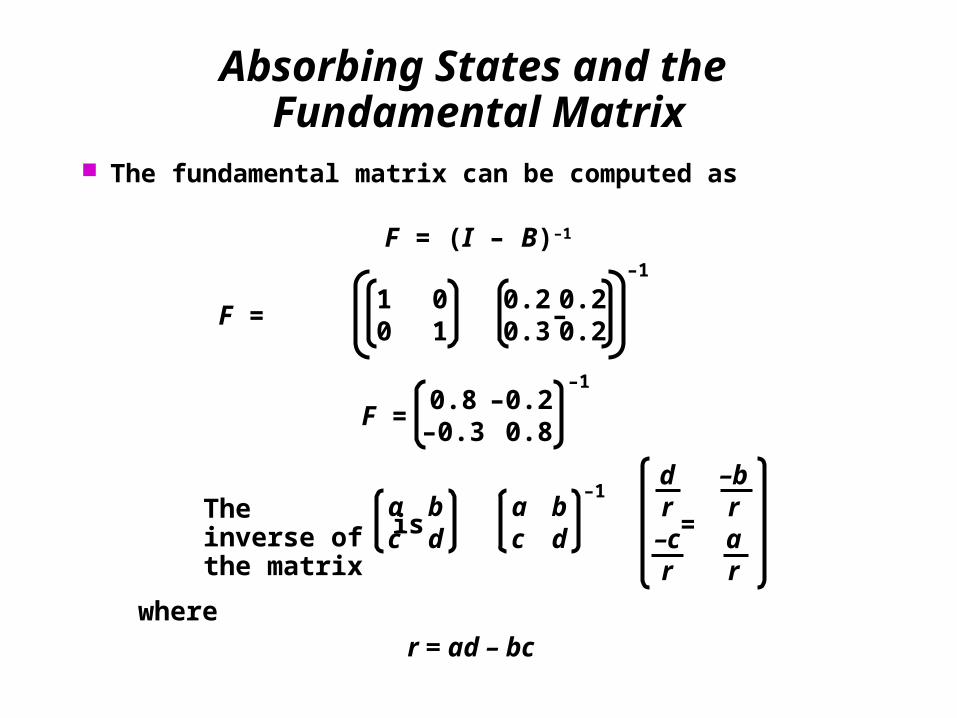
The fundamental matrix can be computed as
F = (I – B)–1
0.8 –0.2–0.3 0.8
F =
–1
The inverse of the matrix
a bc d is =
a bc d
–1d –br r
–c ar r
wherer = ad – bc
0.2 0.20.3 0.2
1 00 1
F = –
–1
Absorbing States and the Fundamental Matrix
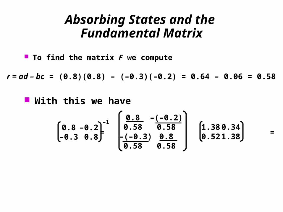
To find the matrix F we compute
r = ad – bc = (0.8)(0.8) – (–0.3)(–0.2) = 0.64 – 0.06 = 0.58
With this we have
0.8 –0.2–0.3 0.8
F = = =
–10.8 –(–0.2)
0.58 0.58–(–0.3) 0.8
0.58 0.58
1.38 0.340.52 1.38
Absorbing States and the Fundamental Matrix
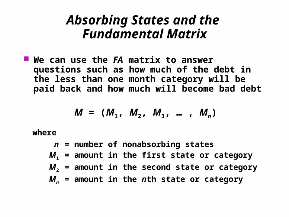
We can use the FA matrix to answer questions such as how much of the debt in the less than one month category will be paid back and how much will become bad debt
M = (M1, M2, M3, … , Mn)
where
n = number of nonabsorbing statesM1 = amount in the first state or category
M2 = amount in the second state or category
Mn = amount in the nth state or category
Absorbing States and the Fundamental Matrix
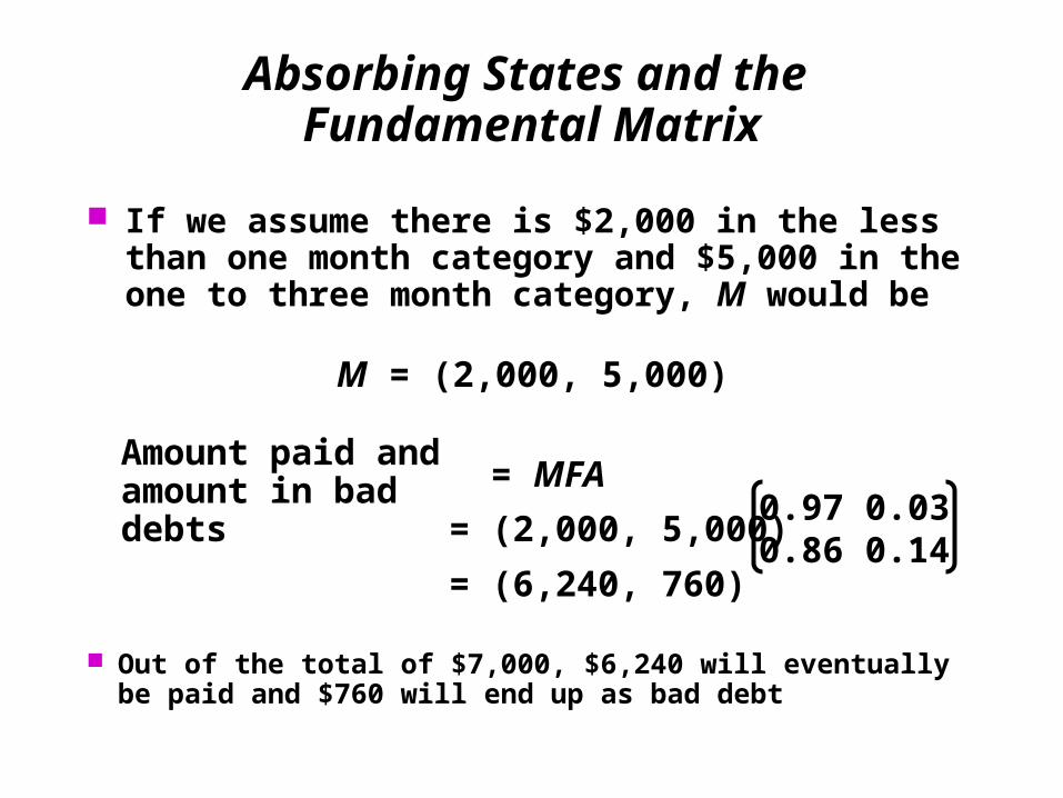
If we assume there is $2,000 in the less than one month category and $5,000 in the one to three month category, M would be
M = (2,000, 5,000)
Amount paid and amount in bad debts = MFA
= (2,000, 5,000)
= (6,240, 760)
0.97 0.030.86 0.14
Out of the total of $7,000, $6,240 will eventually be paid and $760 will end up as bad debt