Embed Size (px)
Citation preview

Chapter ML:VI
VI. Neural Networksq Perceptron Learningq Gradient Descentq Multilayer Perceptronq Radial Basis Functions
ML:VI-1 Neural Networks © STEIN 2005-2018

Perceptron LearningThe Biological Model
Simplified model of a neuron:
cell body
dendrites
synapse
axon
ML:VI-2 Neural Networks © STEIN 2005-2018
Perceptron LearningThe Biological Model (continued)
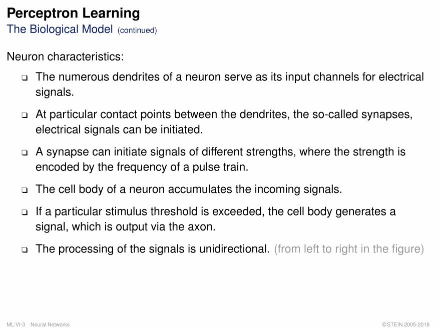
Neuron characteristics:
q The numerous dendrites of a neuron serve as its input channels for electricalsignals.
q At particular contact points between the dendrites, the so-called synapses,electrical signals can be initiated.
q A synapse can initiate signals of different strengths, where the strength isencoded by the frequency of a pulse train.
q The cell body of a neuron accumulates the incoming signals.
q If a particular stimulus threshold is exceeded, the cell body generates asignal, which is output via the axon.
q The processing of the signals is unidirectional. (from left to right in the figure)
ML:VI-3 Neural Networks © STEIN 2005-2018
Perceptron LearningHistory
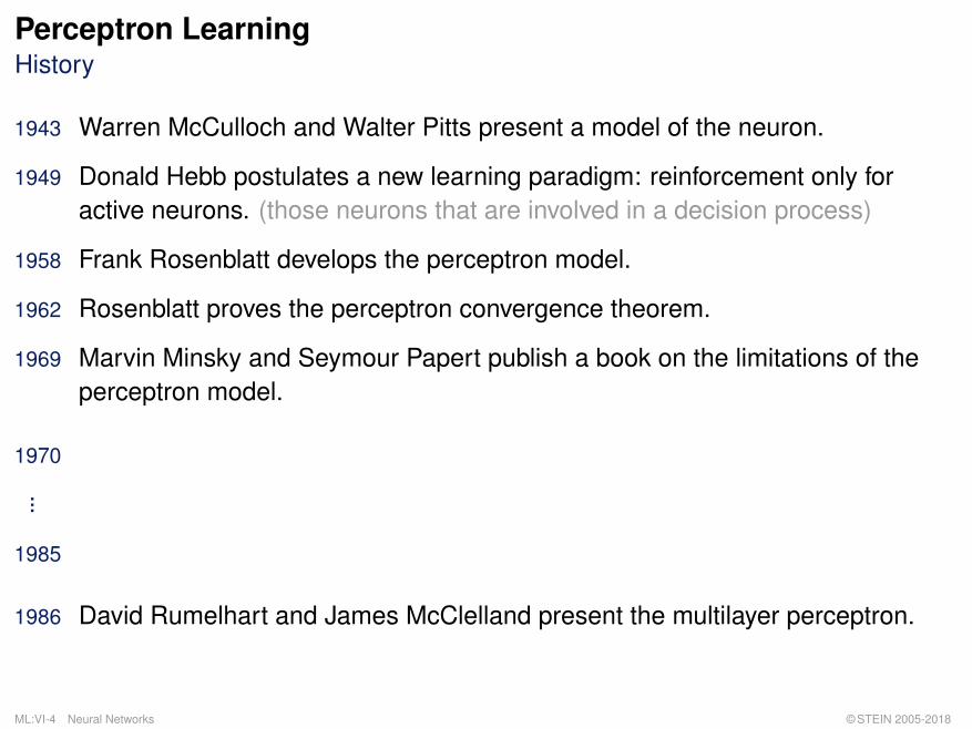
1943 Warren McCulloch and Walter Pitts present a model of the neuron.
1949 Donald Hebb postulates a new learning paradigm: reinforcement only foractive neurons. (those neurons that are involved in a decision process)
1958 Frank Rosenblatt develops the perceptron model.
1962 Rosenblatt proves the perceptron convergence theorem.
1969 Marvin Minsky and Seymour Papert publish a book on the limitations of theperceptron model.
1970
...
1985
1986 David Rumelhart and James McClelland present the multilayer perceptron.
ML:VI-4 Neural Networks © STEIN 2005-2018

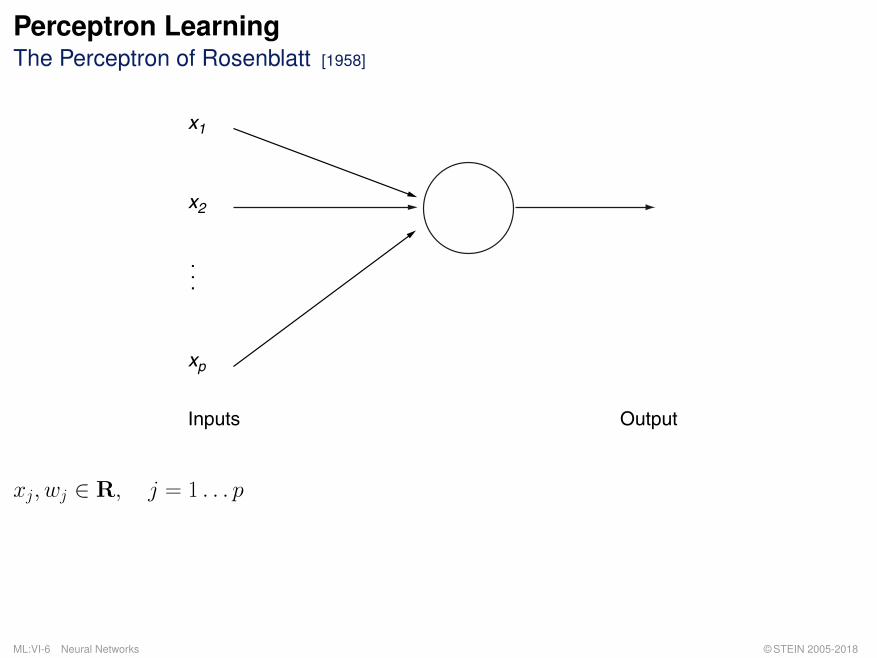
Perceptron LearningThe Perceptron of Rosenblatt [1958]
Inputs Output
ML:VI-5 Neural Networks © STEIN 2005-2018
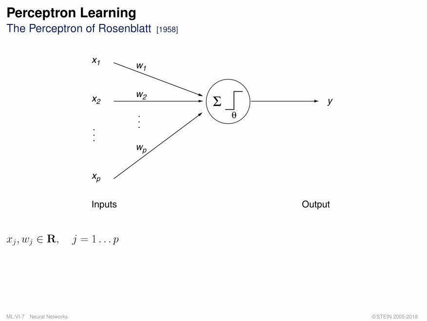
Perceptron LearningThe Perceptron of Rosenblatt [1958]
Inputs Output
xp
.
.
.
x2
x1
xj, wj ∈ R, j = 1 . . . p
ML:VI-6 Neural Networks © STEIN 2005-2018
Perceptron LearningThe Perceptron of Rosenblatt [1958]
Inputs Output
xp
.
.
.
x2
x1
θyΣ
wp
.
.
.
w2
w1
xj, wj ∈ R, j = 1 . . . p
ML:VI-7 Neural Networks © STEIN 2005-2018

Remarks:
q The perceptron of Rosenblatt is based on the neuron model of McCulloch and Pitts.
q The perceptron is a “feed forward system”.
ML:VI-8 Neural Networks © STEIN 2005-2018
Perceptron LearningSpecification of Classification Problems [
::::ML
:::::::::::::Introduction]
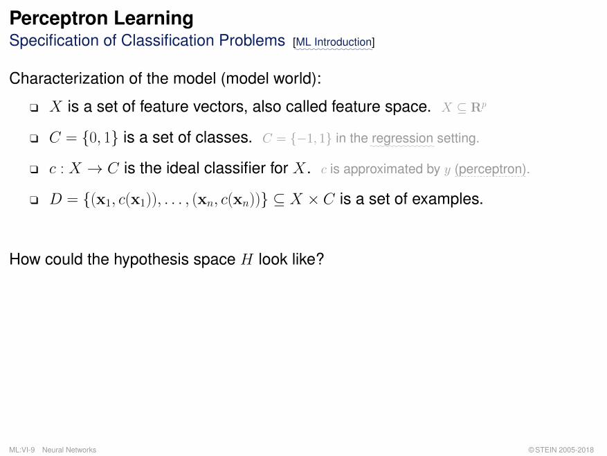
Characterization of the model (model world):
q X is a set of feature vectors, also called feature space. X ⊆ Rp
q C = {0, 1} is a set of classes. C = {−1, 1} in the::::::::::::::regression setting.
q c : X → C is the ideal classifier for X. c is approximated by y (perceptron).
q D = {(x1, c(x1)), . . . , (xn, c(xn))} ⊆ X × C is a set of examples.
How could the hypothesis space H look like?
ML:VI-9 Neural Networks © STEIN 2005-2018

Perceptron LearningComputation in the Perceptron [
::::::::::::Regression]
Ifp∑j=1
wjxj ≥ θ then y(x) = 1, and
ifp∑j=1
wjxj < θ then y(x) = 0.
ML:VI-10 Neural Networks © STEIN 2005-2018

Perceptron LearningComputation in the Perceptron [
::::::::::::Regression]
Ifp∑j=1
wjxj ≥ θ then y(x) = 1, and
ifp∑j=1
wjxj < θ then y(x) = 0.
1
0 Σ wj ×xjj=0
p
θ j=1
wherep∑j=1
wjxj = wTx. (or other notations for the scalar product)
Ü A hypothesis is determined by θ, w1, . . . , wp.
ML:VI-11 Neural Networks © STEIN 2005-2018

Perceptron LearningComputation in the Perceptron (continued)
y(x) = heaviside(
p∑j=1
wjxj − θ)
= heaviside(
p∑j=0
wjxj) with w0 = −θ, x0 = 1
1
0 Σ wj ×xjj=0
p
Inputs Output
xp
.
.
.
x2
x1
θyΣ
wp
.
.
.
w2
w1
0
w0 = −θx0 =1
Ü A hypothesis is determined by w0, w1, . . . , wp.
ML:VI-12 Neural Networks © STEIN 2005-2018
Remarks:
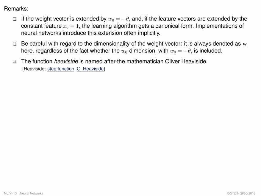
q If the weight vector is extended by w0 = −θ, and, if the feature vectors are extended by theconstant feature x0 = 1, the learning algorithm gets a canonical form. Implementations ofneural networks introduce this extension often implicitly.
q Be careful with regard to the dimensionality of the weight vector: it is always denoted as where, regardless of the fact whether the w0-dimension, with w0 = −θ, is included.
q The function heaviside is named after the mathematician Oliver Heaviside.[Heaviside: step function O. Heaviside]
ML:VI-13 Neural Networks © STEIN 2005-2018

Perceptron LearningWeight Adaptation [IGD Algorithm]
Algorithm: PT Perceptron TrainingInput: D Training examples (x, c(x)) with |x| = p+ 1, c(x) ∈ {0, 1}.
η Learning rate, a small positive constant.Internal: y(D) Set of y(x)-values computed from the elements x in D given some w.Output: w Weight vector.
PT (D, η)
1. initialize_random_weights(w), t = 0
2. REPEAT
3. t = t+ 1
4. (x, c(x)) = random_select(D)
5. error = c(x)− heaviside(wTx) // c(x) ∈ {0, 1}, heaviside ∈ {0, 1}, error ∈ {0, 1,−1}6. ∆w = η · error · x7. w = w + ∆w
8. UNTIL(convergence(D, y(D)) OR t > tmax)
9. return(w)
ML:VI-14 Neural Networks © STEIN 2005-2018
Remarks:
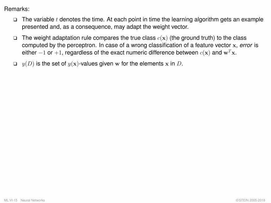
q The variable t denotes the time. At each point in time the learning algorithm gets an examplepresented and, as a consequence, may adapt the weight vector.
q The weight adaptation rule compares the true class c(x) (the ground truth) to the classcomputed by the perceptron. In case of a wrong classification of a feature vector x, error iseither −1 or +1, regardless of the exact numeric difference between c(x) and wTx.
q y(D) is the set of y(x)-values given w for the elements x in D.
ML:VI-15 Neural Networks © STEIN 2005-2018
Perceptron LearningWeight Adaptation: Illustration in Input Space
x2
x1
n
x2
x1
n
d
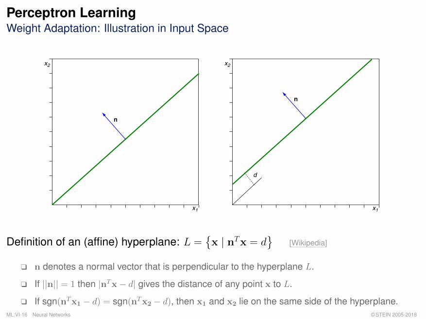
Definition of an (affine) hyperplane: L ={x | nTx = d
}[Wikipedia]
q n denotes a normal vector that is perpendicular to the hyperplane L.
q If ||n|| = 1 then |nTx− d| gives the distance of any point x to L.
q If sgn(nTx1 − d) = sgn(nTx2 − d), then x1 and x2 lie on the same side of the hyperplane.ML:VI-16 Neural Networks © STEIN 2005-2018

Perceptron LearningWeight Adaptation: Illustration in Input Space (continued)
x2
x1
(w1,...,wp)T
x2
x1
θ
Definition of an (affine) hyperplane: wTx = 0 ⇔p∑j=1
wjxj = θ = −w0
(hyperplane definition as before, with notation taken from the classification problem setting)
ML:VI-17 Neural Networks © STEIN 2005-2018
Remarks:
q A perceptron defines a hyperplane that is perpendicular (= normal) to (w1, . . . , wp)T .
q θ or −w0 specify the offset of the hyperplane from the origin, along (w1, . . . , wp)T and as
multiple of 1/||(w1, . . . , wp)T ||.
q The set of possible weight vectors w = (w0, w1, . . . , wp)T form the hypothesis space H.
q Weight adaptation means learning, and the shown learning paradigm is supervised.
q For the weight adaptation in Line 6–7 of the PT Algorithm, note that if some xj is zero, ∆wjwill be zero as well. Keyword: Hebbian learning [Hebb 1949]
q Note that here (and in the following illustrations) the hyperplane movement is not the result ofsolving a regression problem in the (p+ 1)-dimensional input-output-space, where theresiduals are to be minimized. Instead, the PT Algorithm takes each missclassified exampleas a trigger to correct the hyperplane’s normal vector—without taking the effect on the otherresiduals into account.
ML:VI-18 Neural Networks © STEIN 2005-2018

Perceptron LearningExample
A
B
q The examples are presented to the perceptron.
q The perceptron computes a value that is interpreted as class label.
ML:VI-19 Neural Networks © STEIN 2005-2018
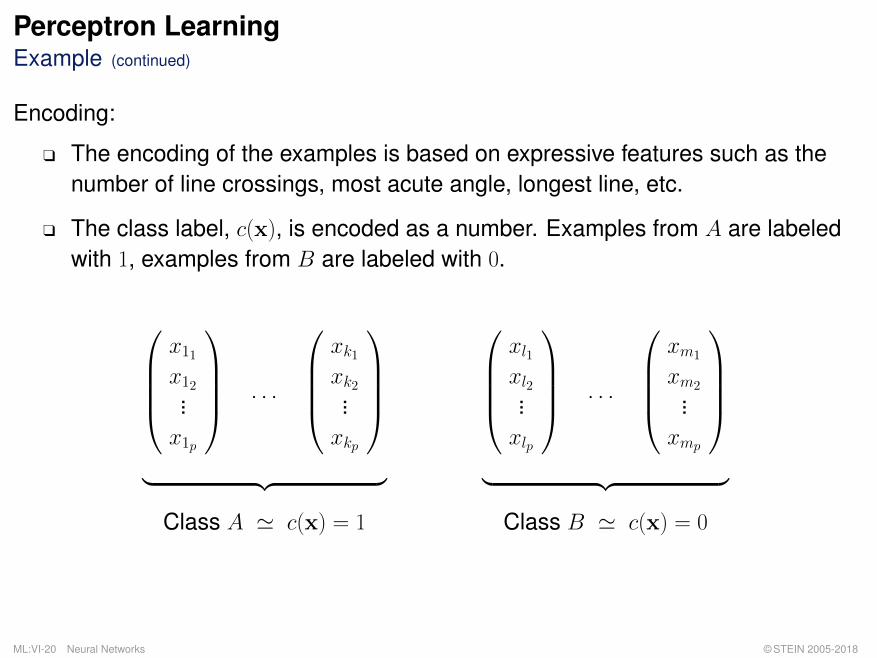
Perceptron LearningExample (continued)
Encoding:
q The encoding of the examples is based on expressive features such as thenumber of line crossings, most acute angle, longest line, etc.
q The class label, c(x), is encoded as a number. Examples from A are labeledwith 1, examples from B are labeled with 0.
x11
x12...x1p
. . .
xk1xk2...xkp
︸ ︷︷ ︸
Class A ' c(x) = 1
xl1xl2...xlp
. . .
xm1
xm2...xmp
︸ ︷︷ ︸
Class B ' c(x) = 0
ML:VI-20 Neural Networks © STEIN 2005-2018
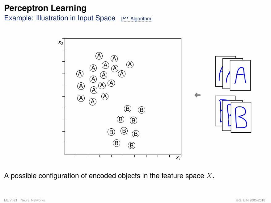
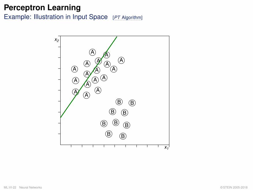
Perceptron LearningExample: Illustration in Input Space [PT Algorithm]
A
x2
x1
A
B
A
A
A
A AA
A
A
A
B
B
B
B
B
B
BB
A
AA
AA
A
�
A possible configuration of encoded objects in the feature space X.
ML:VI-21 Neural Networks © STEIN 2005-2018
Perceptron LearningExample: Illustration in Input Space [PT Algorithm]
A
x2
x1
A
B
A
A
A
A AA
A
A
A
B
B
B
B
B
B
BB
A
AA
AA
A
ML:VI-22 Neural Networks © STEIN 2005-2018
Perceptron LearningExample: Illustration in Input Space [PT Algorithm]
A
x2
x1
A
B
A
A
A
A AA
A
A
A
B
B
B
B
B
B
BB
A
AA
AA
A
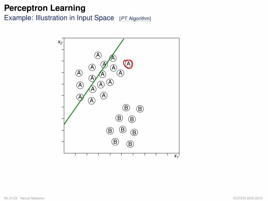
ML:VI-23 Neural Networks © STEIN 2005-2018

Perceptron LearningExample: Illustration in Input Space [PT Algorithm]
A
x2
x1
A
B
A
A
A
A AA
A
A
A
B
B
B
B
B
B
BB
A
AA
AA
A
(w1,...,wp)T
x
ML:VI-24 Neural Networks © STEIN 2005-2018

Perceptron LearningExample: Illustration in Input Space [PT Algorithm]
A
x2
x1
A
B
A
A
A
A AA
A
A
A
B
B
B
B
B
B
BB
A
AA
AA
A
ML:VI-25 Neural Networks © STEIN 2005-2018
Perceptron LearningExample: Illustration in Input Space [PT Algorithm]
A
x2
x1
A
B
A
A
A
A AA
A
A
A
B
B
B
B
B
B
BB
A
AA
AA
A
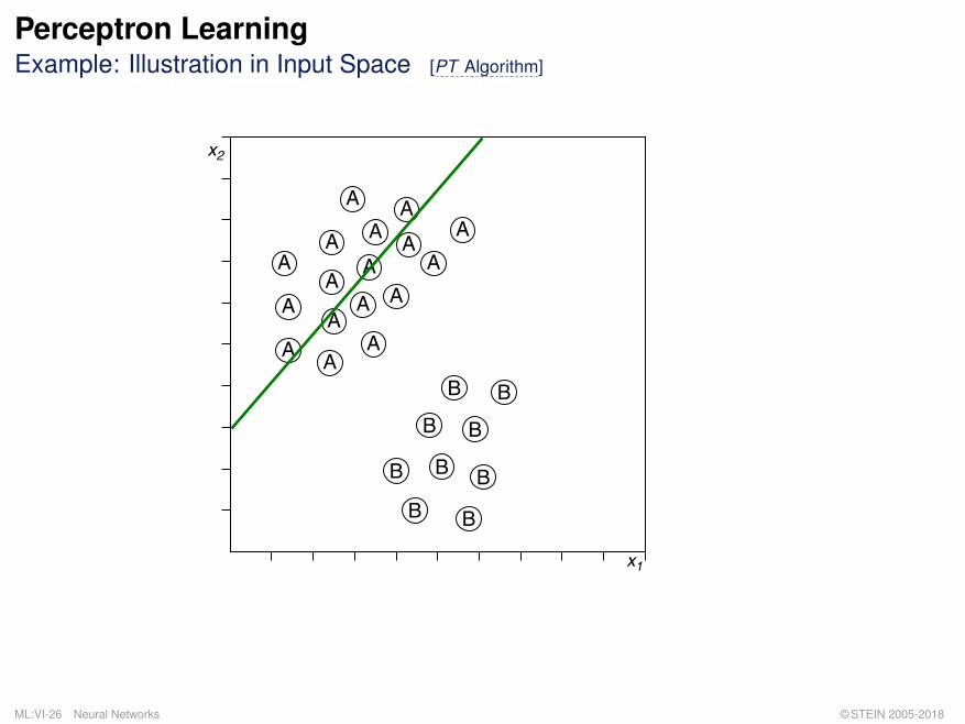
ML:VI-26 Neural Networks © STEIN 2005-2018

Perceptron LearningExample: Illustration in Input Space [PT Algorithm]
A
x2
x1
A
B
A
A
A
A AA
A
A
A
B
B
B
B
B
B
BB
A
AA
AA
A
ML:VI-27 Neural Networks © STEIN 2005-2018

Perceptron LearningExample: Illustration in Input Space [PT Algorithm]
A
x2
x1
A
B
A
A
A
A AA
A
A
A
B
B
B
B
B
B
BB
A
AA
AA
A
ML:VI-28 Neural Networks © STEIN 2005-2018

Perceptron LearningExample: Illustration in Input Space [PT Algorithm]
A
x2
x1
A
B
A
A
A
A AA
A
A
A
B
B
B
B
B
B
BB
A
AA
AA
A
ML:VI-29 Neural Networks © STEIN 2005-2018
Perceptron LearningExample: Illustration in Input Space [PT Algorithm]
A
x2
x1
A
B
A
A
A
A AA
A
A
A
B
B
B
B
B
B
BB
A
AA
AA
A
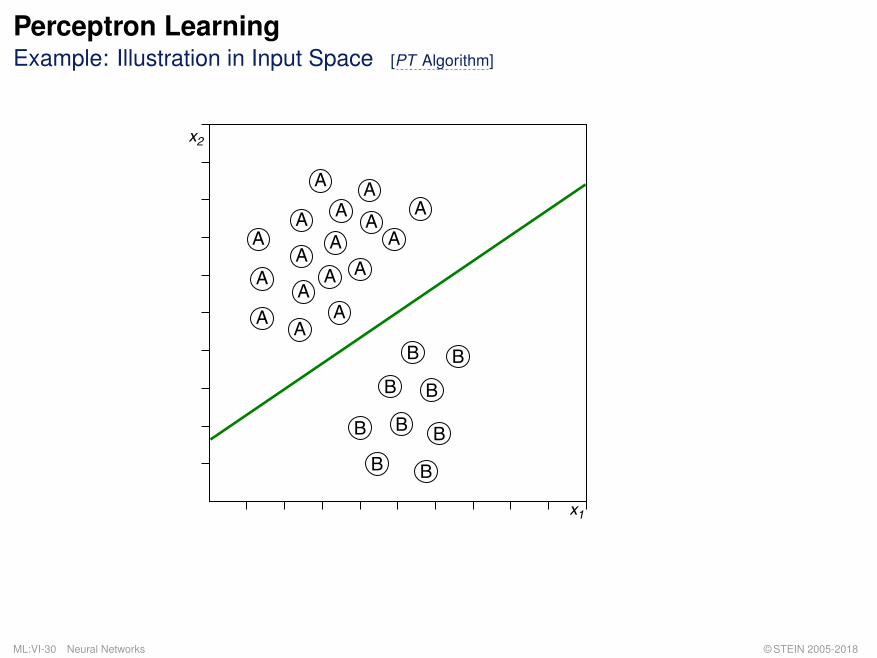
ML:VI-30 Neural Networks © STEIN 2005-2018

Perceptron LearningPerceptron Convergence Theorem
Questions:
1. Which kind of learning tasks can be addressed with the functions in thehypothesis space H?
2. Can the PT Algorithm construct such a function for a given task?
ML:VI-31 Neural Networks © STEIN 2005-2018

Perceptron LearningPerceptron Convergence Theorem
Questions:
1. Which kind of learning tasks can be addressed with the functions in thehypothesis space H?
2. Can the PT Algorithm construct such a function for a given task?
Theorem 1 (Perceptron Convergence [Rosenblatt 1962])
Let X0 and X1 be two finite sets with vectors of the form x = (1, x1, . . . , xp)T , let
X1 ∩X0 = ∅, and let w define a separating hyperplane with respect to X0 and X1.Moreover, let D be a set of examples of the form (x, 0), x ∈ X0 and (x, 1), x ∈ X1.Then holds:
If the examples in D are processed with the PT Algorithm, the constructed weightvector w will converge within a finite number of iterations.
ML:VI-32 Neural Networks © STEIN 2005-2018
Perceptron LearningPerceptron Convergence Theorem: Proof
Preliminaries:q The sets X1 and X0 are separated by a hyperplane w. The proof requires that for all x ∈ X1
the inequality wTx > 0 holds. This condition is always fulfilled, as the following considerationshows.Let x′ ∈ X1 with wTx′ = 0. Since X0 is finite, the members x ∈ X0 have a minimum positivedistance δ with regard to the hyperplane w. Hence, w can be moved by δ
2 towards X0,resulting in a new hyperplane w′ that still fulfills (w′)Tx < 0 for all x ∈ X0, but that now alsofulfills (w′)Tx > 0 for all x ∈ X1.
ML:VI-33 Neural Networks © STEIN 2005-2018
Perceptron LearningPerceptron Convergence Theorem: Proof
Preliminaries:q The sets X1 and X0 are separated by a hyperplane w. The proof requires that for all x ∈ X1
the inequality wTx > 0 holds. This condition is always fulfilled, as the following considerationshows.Let x′ ∈ X1 with wTx′ = 0. Since X0 is finite, the members x ∈ X0 have a minimum positivedistance δ with regard to the hyperplane w. Hence, w can be moved by δ
2 towards X0,resulting in a new hyperplane w′ that still fulfills (w′)Tx < 0 for all x ∈ X0, but that now alsofulfills (w′)Tx > 0 for all x ∈ X1.
q By defining X ′ = X1 ∪ {−x | x ∈ X0}, the searched w fulfills wTx > 0 for all x ∈ X ′. Then,with c(x) = 1 for all x ∈ X ′, error ∈ {0, 1} (instead of {0, 1,−1}). [PT Algorithm, Line 5]
ML:VI-34 Neural Networks © STEIN 2005-2018
Perceptron LearningPerceptron Convergence Theorem: Proof
Preliminaries:q The sets X1 and X0 are separated by a hyperplane w. The proof requires that for all x ∈ X1
the inequality wTx > 0 holds. This condition is always fulfilled, as the following considerationshows.Let x′ ∈ X1 with wTx′ = 0. Since X0 is finite, the members x ∈ X0 have a minimum positivedistance δ with regard to the hyperplane w. Hence, w can be moved by δ
2 towards X0,resulting in a new hyperplane w′ that still fulfills (w′)Tx < 0 for all x ∈ X0, but that now alsofulfills (w′)Tx > 0 for all x ∈ X1.
q By defining X ′ = X1 ∪ {−x | x ∈ X0}, the searched w fulfills wTx > 0 for all x ∈ X ′. Then,with c(x) = 1 for all x ∈ X ′, error ∈ {0, 1} (instead of {0, 1,−1}). [PT Algorithm, Line 5]
q The PT Algorithm performs a number of iterations, where w(t) denotes the weight vector foriteration t, which form the basis for the weight vector w(t+ 1). x(t) ∈ X ′ denotes the featurevector chosen in round t. The first (and randomly chosen) weight vector is denoted as w(0).
ML:VI-35 Neural Networks © STEIN 2005-2018
Perceptron LearningPerceptron Convergence Theorem: Proof
Preliminaries:q The sets X1 and X0 are separated by a hyperplane w. The proof requires that for all x ∈ X1
the inequality wTx > 0 holds. This condition is always fulfilled, as the following considerationshows.Let x′ ∈ X1 with wTx′ = 0. Since X0 is finite, the members x ∈ X0 have a minimum positivedistance δ with regard to the hyperplane w. Hence, w can be moved by δ
2 towards X0,resulting in a new hyperplane w′ that still fulfills (w′)Tx < 0 for all x ∈ X0, but that now alsofulfills (w′)Tx > 0 for all x ∈ X1.
q By defining X ′ = X1 ∪ {−x | x ∈ X0}, the searched w fulfills wTx > 0 for all x ∈ X ′. Then,with c(x) = 1 for all x ∈ X ′, error ∈ {0, 1} (instead of {0, 1,−1}). [PT Algorithm, Line 5]
q The PT Algorithm performs a number of iterations, where w(t) denotes the weight vector foriteration t, which form the basis for the weight vector w(t+ 1). x(t) ∈ X ′ denotes the featurevector chosen in round t. The first (and randomly chosen) weight vector is denoted as w(0).
q Recall the Cauchy-Schwarz inequality: ||a||2 · ||b||2 ≥ (aTb)2, where ||x|| :=√xTx denotes
the Euclidean norm.
ML:VI-36 Neural Networks © STEIN 2005-2018
Perceptron LearningPerceptron Convergence Theorem: Proof (continued)
Line of argument:(a) We state a lower bound for how much ||w|| must change from its initial value after n iterations
(to become a separating hyperplane). The derivation of this lower bound exploits thepresupposed linear separability of X0 and X1.
(b) We state an upper bound for how much ||w|| can change from its initial value after n iterations.The derivation of this upper bound exploits the finiteness of X0 and X1, which in turnguarantees the existence of an upper bound for the norm of the maximum feature vector.
(c) We observe that the lower bound grows quadratically in n, whereas the upper bound growslinearly. From the relation “lower bound < upper bound” we derive a finite upper bound for n.
ML:VI-37 Neural Networks © STEIN 2005-2018
Perceptron LearningPerceptron Convergence Theorem: Proof (continued)
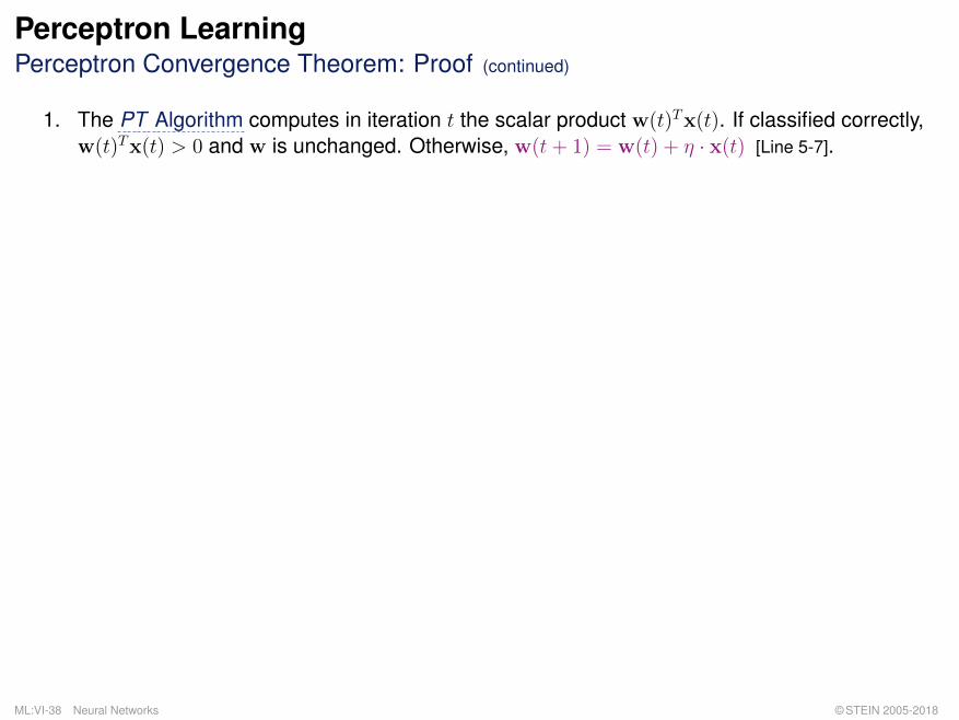
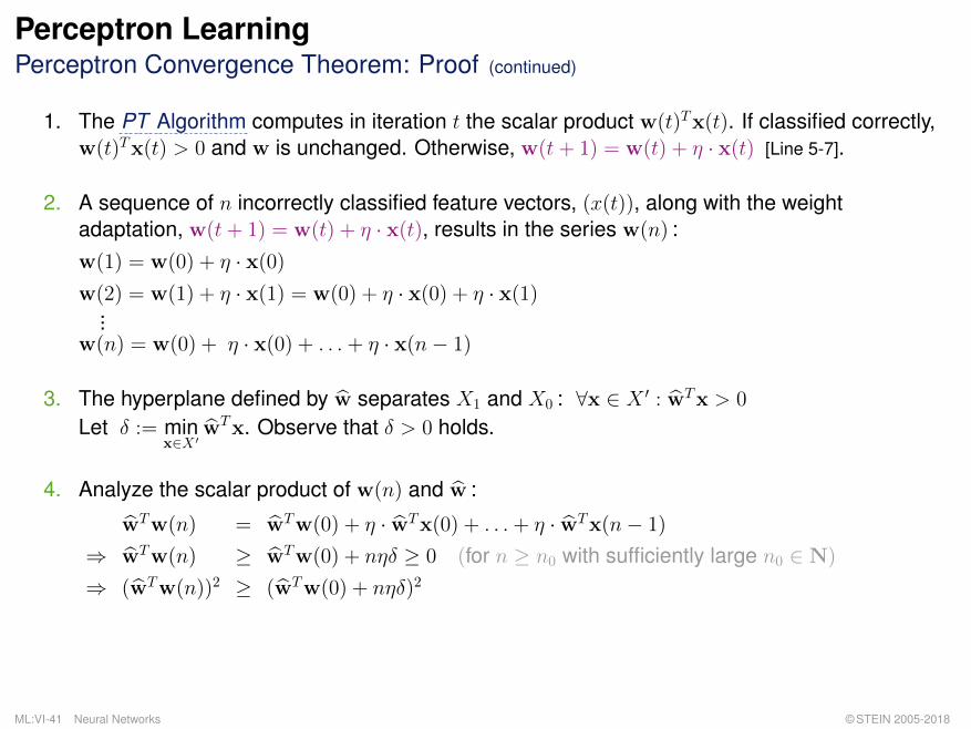
1. The PT Algorithm computes in iteration t the scalar product w(t)Tx(t). If classified correctly,w(t)Tx(t) > 0 and w is unchanged. Otherwise, w(t+ 1) = w(t) + η · x(t) [Line 5-7].
ML:VI-38 Neural Networks © STEIN 2005-2018
Perceptron LearningPerceptron Convergence Theorem: Proof (continued)
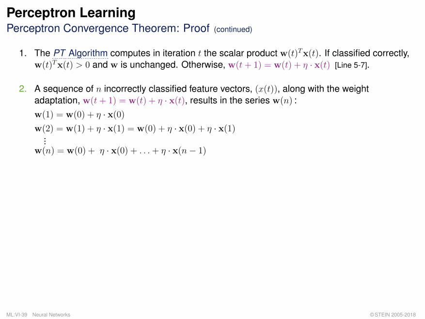
1. The PT Algorithm computes in iteration t the scalar product w(t)Tx(t). If classified correctly,w(t)Tx(t) > 0 and w is unchanged. Otherwise, w(t+ 1) = w(t) + η · x(t) [Line 5-7].
2. A sequence of n incorrectly classified feature vectors, (x(t)), along with the weightadaptation, w(t+ 1) = w(t) + η · x(t), results in the series w(n) :w(1) = w(0) + η · x(0)
w(2) = w(1) + η · x(1) = w(0) + η · x(0) + η · x(1)...
w(n) = w(0) + η · x(0) + . . .+ η · x(n− 1)
ML:VI-39 Neural Networks © STEIN 2005-2018

Perceptron LearningPerceptron Convergence Theorem: Proof (continued)
1. The PT Algorithm computes in iteration t the scalar product w(t)Tx(t). If classified correctly,w(t)Tx(t) > 0 and w is unchanged. Otherwise, w(t+ 1) = w(t) + η · x(t) [Line 5-7].
2. A sequence of n incorrectly classified feature vectors, (x(t)), along with the weightadaptation, w(t+ 1) = w(t) + η · x(t), results in the series w(n) :w(1) = w(0) + η · x(0)
w(2) = w(1) + η · x(1) = w(0) + η · x(0) + η · x(1)...
w(n) = w(0) + η · x(0) + . . .+ η · x(n− 1)
3. The hyperplane defined by w separates X1 and X0 : ∀x ∈ X ′ : wTx > 0
Let δ := minx∈X ′
wTx. Observe that δ > 0 holds.
ML:VI-40 Neural Networks © STEIN 2005-2018
Perceptron LearningPerceptron Convergence Theorem: Proof (continued)
1. The PT Algorithm computes in iteration t the scalar product w(t)Tx(t). If classified correctly,w(t)Tx(t) > 0 and w is unchanged. Otherwise, w(t+ 1) = w(t) + η · x(t) [Line 5-7].
2. A sequence of n incorrectly classified feature vectors, (x(t)), along with the weightadaptation, w(t+ 1) = w(t) + η · x(t), results in the series w(n) :w(1) = w(0) + η · x(0)
w(2) = w(1) + η · x(1) = w(0) + η · x(0) + η · x(1)...
w(n) = w(0) + η · x(0) + . . .+ η · x(n− 1)
3. The hyperplane defined by w separates X1 and X0 : ∀x ∈ X ′ : wTx > 0
Let δ := minx∈X ′
wTx. Observe that δ > 0 holds.
4. Analyze the scalar product of w(n) and w :
wTw(n) = wTw(0) + η · wTx(0) + . . .+ η · wTx(n− 1)
⇒ wTw(n) ≥ wTw(0) + nηδ ≥ 0 (for n ≥ n0 with sufficiently large n0 ∈ N)
⇒ (wTw(n))2 ≥ (wTw(0) + nηδ)2
ML:VI-41 Neural Networks © STEIN 2005-2018
Perceptron LearningPerceptron Convergence Theorem: Proof (continued)
1. The PT Algorithm computes in iteration t the scalar product w(t)Tx(t). If classified correctly,w(t)Tx(t) > 0 and w is unchanged. Otherwise, w(t+ 1) = w(t) + η · x(t) [Line 5-7].
2. A sequence of n incorrectly classified feature vectors, (x(t)), along with the weightadaptation, w(t+ 1) = w(t) + η · x(t), results in the series w(n) :w(1) = w(0) + η · x(0)
w(2) = w(1) + η · x(1) = w(0) + η · x(0) + η · x(1)...
w(n) = w(0) + η · x(0) + . . .+ η · x(n− 1)
3. The hyperplane defined by w separates X1 and X0 : ∀x ∈ X ′ : wTx > 0
Let δ := minx∈X ′
wTx. Observe that δ > 0 holds.
4. Analyze the scalar product of w(n) and w :
wTw(n) = wTw(0) + η · wTx(0) + . . .+ η · wTx(n− 1)
⇒ wTw(n) ≥ wTw(0) + nηδ ≥ 0 (for n ≥ n0 with sufficiently large n0 ∈ N)
⇒ (wTw(n))2 ≥ (wTw(0) + nηδ)2
5. Apply the Cauchy-Schwarz inequality:
||w||2 · ||w(n)||2 ≥ (wTw(0) + nηδ)2 ⇒ ||w(n)||2 ≥ (wTw(0) + nηδ)2
||w||2ML:VI-42 Neural Networks © STEIN 2005-2018

Perceptron LearningPerceptron Convergence Theorem: Proof (continued)
6. Consider again the weight adaptation w(t+ 1) = w(t) + η · x(t) :
||w(t+ 1)||2 = ||w(t) + η · x(t)||2
= (w(t) + η · x(t))T (w(t) + η · x(t))
= w(t)Tw(t) + η2 · x(t)Tx(t) + 2η ·w(t)Tx(t)
≤ ||w(t)||2 + ||η · x(t)||2 (since w(t)Tx(t) < 0)
ML:VI-43 Neural Networks © STEIN 2005-2018
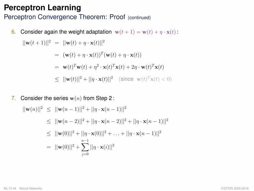
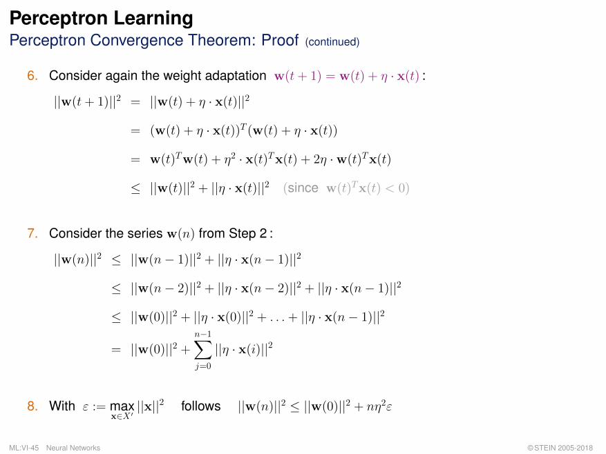
Perceptron LearningPerceptron Convergence Theorem: Proof (continued)
6. Consider again the weight adaptation w(t+ 1) = w(t) + η · x(t) :
||w(t+ 1)||2 = ||w(t) + η · x(t)||2
= (w(t) + η · x(t))T (w(t) + η · x(t))
= w(t)Tw(t) + η2 · x(t)Tx(t) + 2η ·w(t)Tx(t)
≤ ||w(t)||2 + ||η · x(t)||2 (since w(t)Tx(t) < 0)
7. Consider the series w(n) from Step 2 :
||w(n)||2 ≤ ||w(n− 1)||2 + ||η · x(n− 1)||2
≤ ||w(n− 2)||2 + ||η · x(n− 2)||2 + ||η · x(n− 1)||2
≤ ||w(0)||2 + ||η · x(0)||2 + . . .+ ||η · x(n− 1)||2
= ||w(0)||2 +n−1∑j=0
||η · x(i)||2
ML:VI-44 Neural Networks © STEIN 2005-2018
Perceptron LearningPerceptron Convergence Theorem: Proof (continued)
6. Consider again the weight adaptation w(t+ 1) = w(t) + η · x(t) :
||w(t+ 1)||2 = ||w(t) + η · x(t)||2
= (w(t) + η · x(t))T (w(t) + η · x(t))
= w(t)Tw(t) + η2 · x(t)Tx(t) + 2η ·w(t)Tx(t)
≤ ||w(t)||2 + ||η · x(t)||2 (since w(t)Tx(t) < 0)
7. Consider the series w(n) from Step 2 :
||w(n)||2 ≤ ||w(n− 1)||2 + ||η · x(n− 1)||2
≤ ||w(n− 2)||2 + ||η · x(n− 2)||2 + ||η · x(n− 1)||2
≤ ||w(0)||2 + ||η · x(0)||2 + . . .+ ||η · x(n− 1)||2
= ||w(0)||2 +n−1∑j=0
||η · x(i)||2
8. With ε := maxx∈X ′||x||2 follows ||w(n)||2 ≤ ||w(0)||2 + nη2ε
ML:VI-45 Neural Networks © STEIN 2005-2018

Perceptron LearningPerceptron Convergence Theorem: Proof (continued)
9. Both inequalities (see Step 5 and Step 8) must be fulfilled:
||w(n)||2 ≥ (wTw(0) + nηδ)2
||w||2and ||w(n)||2 ≤ ||w(0)||2 + nη2ε
⇒ (wTw(0) + nηδ)2
||w||2≤ ||w(n)||2 ≤ ||w(0)||2 + nη2ε
⇒ (wTw(0) + nηδ)2
||w||2≤ ||w(0)||2 + nη2ε
Set w(0) = 0 : ⇒ n2η2δ2
||w||2≤ nη2ε
⇔ n ≤ ε
δ2· ||w||2
ML:VI-46 Neural Networks © STEIN 2005-2018

Perceptron LearningPerceptron Convergence Theorem: Proof (continued)
9. Both inequalities (see Step 5 and Step 8) must be fulfilled:
||w(n)||2 ≥ (wTw(0) + nηδ)2
||w||2and ||w(n)||2 ≤ ||w(0)||2 + nη2ε
⇒ (wTw(0) + nηδ)2
||w||2≤ ||w(n)||2 ≤ ||w(0)||2 + nη2ε
⇒ (wTw(0) + nηδ)2
||w||2≤ ||w(0)||2 + nη2ε
Set w(0) = 0 : ⇒ n2η2δ2
||w||2≤ nη2ε
⇔ n ≤ ε
δ2· ||w||2
Ü The PT Algorithm terminates within a finite number of iterations.
Observe:(wTw(0) + nηδ)2
||w||2∈ Θ(n2) and ||w(0)||2 + nη2ε ∈ Θ(n)
ML:VI-47 Neural Networks © STEIN 2005-2018
Perceptron LearningPerceptron Convergence Theorem: Discussion
q If a separating hyperplane between X0 and X1 exists, the PT Algorithm willconverge. If no such hyperplane exists, convergence cannot be guaranteed.
q A separating hyperplane can be found in polynomial time with linearprogramming. The PT Algorithm, however, may require an exponentialnumber of iterations.
ML:VI-48 Neural Networks © STEIN 2005-2018

Perceptron LearningPerceptron Convergence Theorem: Discussion
q If a separating hyperplane between X0 and X1 exists, the PT Algorithm willconverge. If no such hyperplane exists, convergence cannot be guaranteed.
q A separating hyperplane can be found in polynomial time with linearprogramming. The PT Algorithm, however, may require an exponentialnumber of iterations.
q Classification problems with noise (right-hand side) are problematic:
A
x2
x1
A
B
A
A
A
A AA
A
A
A
B
B
B
B
B
B
BB
A
AA
AA
A
A
x2
x1
A
B
A
A
A
A AA
A
A
A
B
B
B
B
B
B
BB
A
AA
AA
A B
B
B
B
B
B
B
BB
ML:VI-49 Neural Networks © STEIN 2005-2018

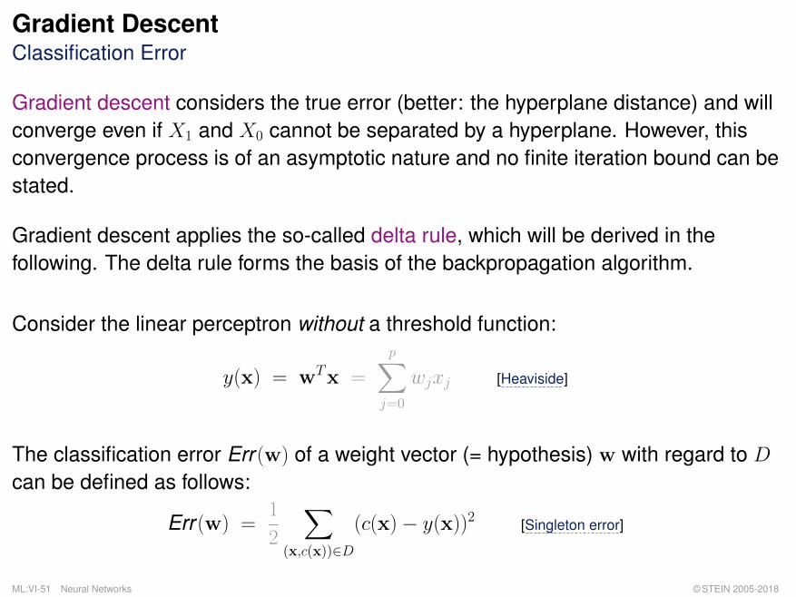
Gradient DescentClassification Error
Gradient descent considers the true error (better: the hyperplane distance) and willconverge even if X1 and X0 cannot be separated by a hyperplane. However, thisconvergence process is of an asymptotic nature and no finite iteration bound can bestated.
Gradient descent applies the so-called delta rule, which will be derived in thefollowing. The delta rule forms the basis of the backpropagation algorithm.
ML:VI-50 Neural Networks © STEIN 2005-2018
Gradient DescentClassification Error
Gradient descent considers the true error (better: the hyperplane distance) and willconverge even if X1 and X0 cannot be separated by a hyperplane. However, thisconvergence process is of an asymptotic nature and no finite iteration bound can bestated.
Gradient descent applies the so-called delta rule, which will be derived in thefollowing. The delta rule forms the basis of the backpropagation algorithm.
Consider the linear perceptron without a threshold function:
y(x) = wTx =
p∑j=0
wjxj [Heaviside]
The classification error Err (w) of a weight vector (= hypothesis) w with regard to Dcan be defined as follows:
Err (w) =1
2
∑(x,c(x))∈D
(c(x)− y(x))2 [Singleton error]
ML:VI-51 Neural Networks © STEIN 2005-2018
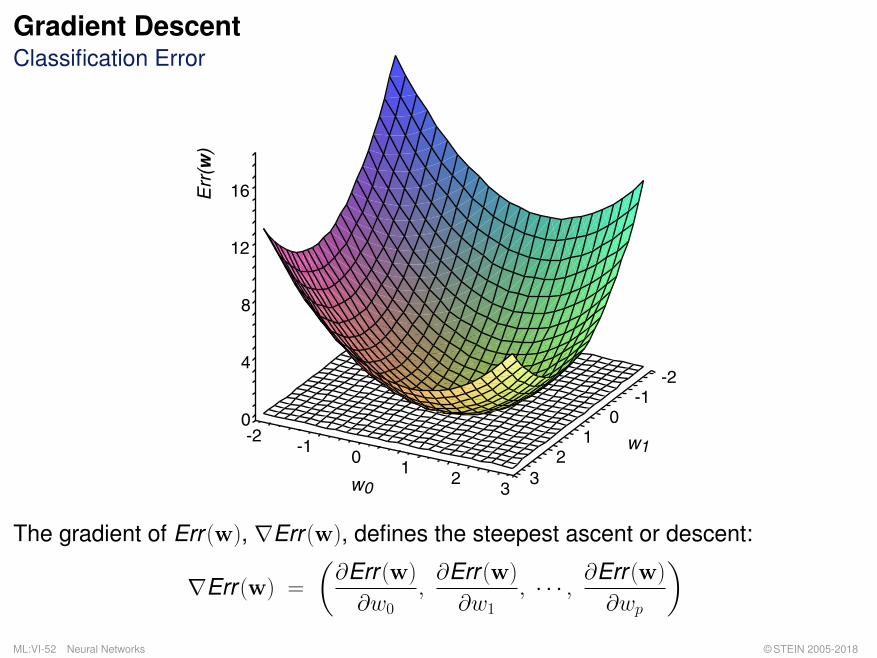
Gradient DescentClassification Error
-2-1
0-2
0w1-1
4
10
8
12
12
w02
16
33
Err
(w)
The gradient of Err (w), ∇Err (w), defines the steepest ascent or descent:
∇Err (w) =
(∂Err (w)
∂w0,∂Err (w)
∂w1, · · · , ∂Err (w)
∂wp
)ML:VI-52 Neural Networks © STEIN 2005-2018
Gradient DescentWeight Adaptation
w ← w + ∆w where ∆w = −η∇Err (w)
Componentwise (j = 0, . . . , p) weight adaptation [PT Algorithm] :
wj ← wj + ∆wj where ∆wj = −η ∂
∂wjErr (w) = η
∑(x, c(x))∈D
(c(x)−wTx) · xj
ML:VI-53 Neural Networks © STEIN 2005-2018
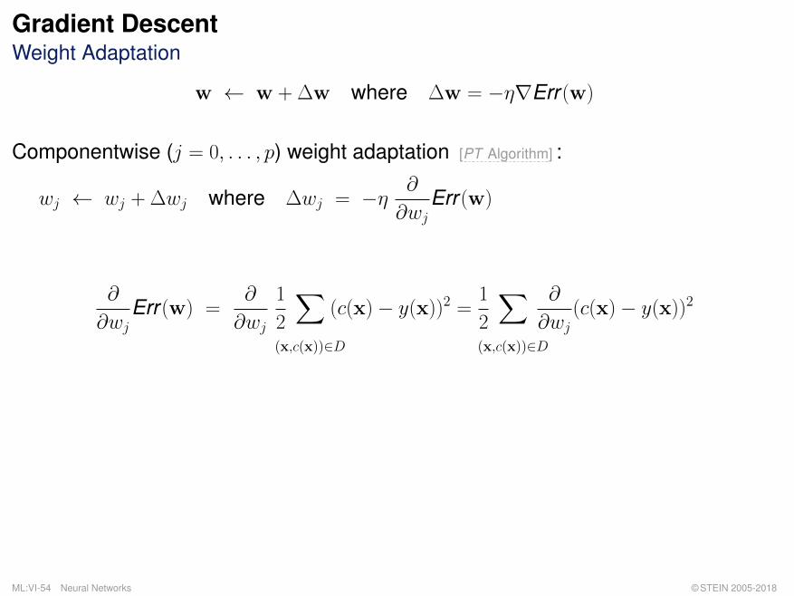
Gradient DescentWeight Adaptation
w ← w + ∆w where ∆w = −η∇Err (w)
Componentwise (j = 0, . . . , p) weight adaptation [PT Algorithm] :
wj ← wj + ∆wj where ∆wj = −η ∂
∂wjErr (w) = η
∑(x, c(x))∈D
(c(x)−wTx) · xj
∂
∂wjErr (w) =
∂
∂wj
1
2
∑(x,c(x))∈D
(c(x)− y(x))2 =1
2
∑(x,c(x))∈D
∂
∂wj(c(x)− y(x))2
=1
2
∑(x,c(x))∈D
2(c(x)− y(x)) · ∂
∂wj(c(x)− y(x))
=∑
(x,c(x))∈D
(c(x)−wTx) · ∂
∂wj(c(x)−wTx)
=∑
(x,c(x))∈D
(c(x)−wTx)(−xj)
ML:VI-54 Neural Networks © STEIN 2005-2018

Gradient DescentWeight Adaptation
w ← w + ∆w where ∆w = −η∇Err (w)
Componentwise (j = 0, . . . , p) weight adaptation [PT Algorithm] :
wj ← wj + ∆wj where ∆wj = −η ∂
∂wjErr (w) = η
∑(x, c(x))∈D
(c(x)−wTx) · xj
∂
∂wjErr (w) =
∂
∂wj
1
2
∑(x,c(x))∈D
(c(x)− y(x))2 =1
2
∑(x,c(x))∈D
∂
∂wj(c(x)− y(x))2
=1
2
∑(x,c(x))∈D
2(c(x)− y(x)) · ∂
∂wj(c(x)− y(x))
=∑
(x,c(x))∈D
(c(x)−wTx) · ∂
∂wj(c(x)−wTx)
=∑
(x,c(x))∈D
(c(x)−wTx)(−xj)
ML:VI-55 Neural Networks © STEIN 2005-2018
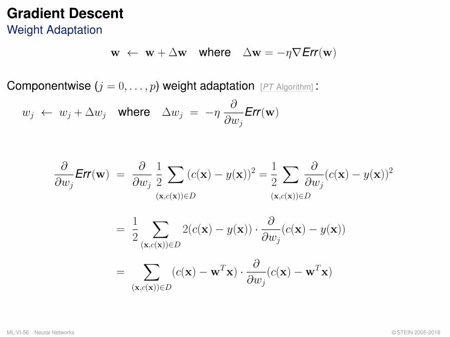
Gradient DescentWeight Adaptation
w ← w + ∆w where ∆w = −η∇Err (w)
Componentwise (j = 0, . . . , p) weight adaptation [PT Algorithm] :
wj ← wj + ∆wj where ∆wj = −η ∂
∂wjErr (w) = η
∑(x, c(x))∈D
(c(x)−wTx) · xj
∂
∂wjErr (w) =
∂
∂wj
1
2
∑(x,c(x))∈D
(c(x)− y(x))2 =1
2
∑(x,c(x))∈D
∂
∂wj(c(x)− y(x))2
=1
2
∑(x,c(x))∈D
2(c(x)− y(x)) · ∂
∂wj(c(x)− y(x))
=∑
(x,c(x))∈D
(c(x)−wTx) · ∂
∂wj(c(x)−wTx)
=∑
(x,c(x))∈D
(c(x)−wTx)(−xj)
ML:VI-56 Neural Networks © STEIN 2005-2018

Gradient DescentWeight Adaptation
w ← w + ∆w where ∆w = −η∇Err (w)
Componentwise (j = 0, . . . , p) weight adaptation [PT Algorithm] :
wj ← wj + ∆wj where ∆wj = −η ∂
∂wjErr (w) = η
∑(x, c(x))∈D
(c(x)−wTx) · xj
∂
∂wjErr (w) =
∂
∂wj
1
2
∑(x,c(x))∈D
(c(x)− y(x))2 =1
2
∑(x,c(x))∈D
∂
∂wj(c(x)− y(x))2
=1
2
∑(x,c(x))∈D
2(c(x)− y(x)) · ∂
∂wj(c(x)− y(x))
=∑
(x,c(x))∈D
(c(x)−wTx) · ∂
∂wj(c(x)−wTx)
=∑
(x,c(x))∈D
(c(x)−wTx)(−xj)
ML:VI-57 Neural Networks © STEIN 2005-2018
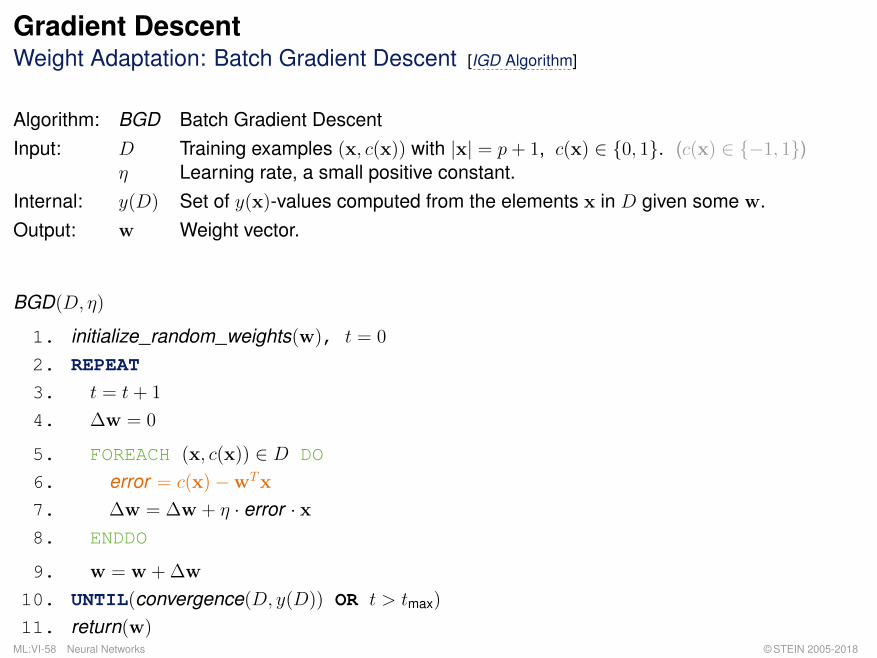
Gradient DescentWeight Adaptation: Batch Gradient Descent [IGD Algorithm]
Algorithm: BGD Batch Gradient DescentInput: D Training examples (x, c(x)) with |x| = p+ 1, c(x) ∈ {0, 1}. (c(x) ∈ {−1, 1})
η Learning rate, a small positive constant.Internal: y(D) Set of y(x)-values computed from the elements x in D given some w.Output: w Weight vector.
BGD(D, η)
1. initialize_random_weights(w), t = 0
2. REPEAT
3. t = t+ 1
4. ∆w = 0
5. FOREACH (x, c(x)) ∈ D DO
6. error = c(x)−wTx
7. ∆w = ∆w + η · error · x8. ENDDO
9. w = w + ∆w
10. UNTIL(convergence(D, y(D)) OR t > tmax)
11. return(w)ML:VI-58 Neural Networks © STEIN 2005-2018
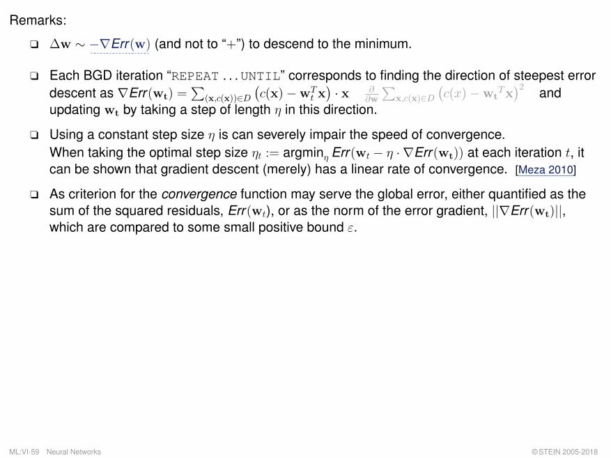
Remarks:
q ∆w ∼ −∇Err(w) (and not to “+”) to descend to the minimum.
q Each BGD iteration “REPEAT . . .UNTIL” corresponds to finding the direction of steepest errordescent as ∇Err(wt) =
∑(x,c(x))∈D
(c(x)−wT
t x)· x ∂
∂w
∑x,c(x)∈D
(c(x)−wt
Tx)2 and
updating wt by taking a step of length η in this direction.
q Using a constant step size η is can severely impair the speed of convergence.When taking the optimal step size ηt := argminη Err(wt − η · ∇Err(wt)) at each iteration t, itcan be shown that gradient descent (merely) has a linear rate of convergence. [Meza 2010]
q As criterion for the convergence function may serve the global error, either quantified as thesum of the squared residuals, Err(wt), or as the norm of the error gradient, ||∇Err(wt)||,which are compared to some small positive bound ε.
ML:VI-59 Neural Networks © STEIN 2005-2018
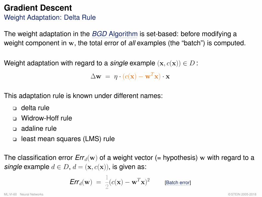
Gradient DescentWeight Adaptation: Delta Rule
The weight adaptation in the BGD Algorithm is set-based: before modifying aweight component in w, the total error of all examples (the “batch”) is computed.
Weight adaptation with regard to a single example (x, c(x)) ∈ D :
∆w = η · (c(x)−wTx) · x
This adaptation rule is known under different names:
q delta ruleq Widrow-Hoff ruleq adaline ruleq least mean squares (LMS) rule
The classification error Err d(w) of a weight vector (= hypothesis) w with regard to asingle example d ∈ D, d = (x, c(x)), is given as:
Err d(w) =1
2(c(x)−wTx)2 [Batch error]
ML:VI-60 Neural Networks © STEIN 2005-2018

Gradient DescentWeight Adaptation: Incremental Gradient Descent [Algorithms:
:::::LMS BGD PT ]
Algorithm: IGD Incremental Gradient DescentInput: D Training examples (x, c(x)) with |x| = p+ 1, c(x) ∈ {0, 1}. (c(x) ∈ {−1, 1})
η Learning rate, a small positive constant.Internal: y(D) Set of y(x)-values computed from the elements x in D given some w.Output: w Weight vector.
IGD(D, η)
1. initialize_random_weights(w), t = 0
2. REPEAT3. t = t+ 1
4. FOREACH (x, c(x)) ∈ D DO
5. error = c(x)−wTx
6. ∆w = η · error · x7. w = w + ∆w
8. ENDDO
9. UNTIL(convergence(D, y(D)) OR t > tmax)
10. return(w)
ML:VI-61 Neural Networks © STEIN 2005-2018
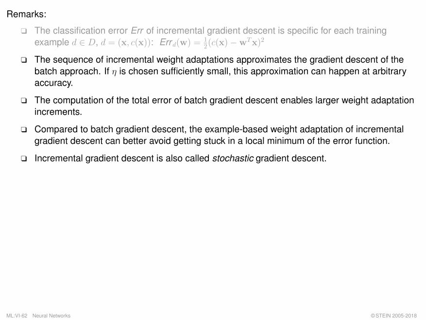
Remarks:
q The classification error Err of incremental gradient descent is specific for each trainingexample d ∈ D, d = (x, c(x)): Err d(w) = 1
2(c(x)−wTx)2
q The sequence of incremental weight adaptations approximates the gradient descent of thebatch approach. If η is chosen sufficiently small, this approximation can happen at arbitraryaccuracy.
q The computation of the total error of batch gradient descent enables larger weight adaptationincrements.
q Compared to batch gradient descent, the example-based weight adaptation of incrementalgradient descent can better avoid getting stuck in a local minimum of the error function.
q Incremental gradient descent is also called stochastic gradient descent.
ML:VI-62 Neural Networks © STEIN 2005-2018

Remarks (continued):
q When, as is done here, the residual sum squares, RSS, is chosen as error (loss) function, theincremental gradient descent algorithm [IGD] corresponds to the least mean squaresalgorithm [
:::::LMS].
q The incremental gradient descend algorithm [IGD] looks similar to the perceptron trainingalgorithm [PT ], since these algorithms differ only in the error computation (Line 5) where thelatter applies the Heaviside function. However, this subtle syntactic difference is a significantconceptual difference, entailing a number of consequences:
– Gradient descent is a regression approach and exploits the residua, which are providedby an error function of choice, and whose differential is evaluated to control thehyperplane movement.
– The PT algorithm is not based on residuals (in the (p+ 1)-dimensional input-output-space) but refers to the input space only, where it simply evaluates the side of thehyperplane as a binary feature (correct side or not).
– Provided linear separability, the PT algorithm will converge within a finite number ofiterations, which, however, cannot be guaranteed for gradient descent.
– Gradient descent will converge even if the data is not linearly separable.
– Data sets can be constructed whose classes are linearly separable, but where gradientdescent will not determine a hyperplane that classifies all examples correctly (whereasthe PT Algorithm of course does).
ML:VI-63 Neural Networks © STEIN 2005-2018