chapter one

Mathematics and Finance

‘Janice! D’ya think you can find that postcard?’ Professor Paul A. Samuelson was in his office at MIT in the Autumn

of 2003 relating how, several decades earlier, he had come across the PhD thesis, dating back to 1900, in which Louis Bachelier had devel­oped a theory of option pricing, a topic that was beginning to occupy Samuelson and other economists in the 1950s. Although no economist at the time had ever heard of Bachelier, he was known in mathematical circles for having independently invented Brownian motion and proved some results about it that appeared in contemporary texts such as J. L. Doob’s famous book Stochastic Processes, published in 1953. William Feller, whose influential two-volume treatise An Introduction to Proba­bility Theory and Its Applications is widely regarded as a masterpiece of twentieth century mathematics, even suggested the alternative name Wiener–Bachelier process for the mathematical process we now know as Brownian motion. The story goes that L. J. (‘Jimmie’) Savage, doyen of mathematical statisticians of the post-World War II era, knew of Bache­lier’s work and, with proselytizing zeal, thought that the economists ought to be told. So he sent postcards to his economist friends warn­ing them that if they had not read Bachelier it was about time they did. Hence Samuelson’s appeal to Janice Murray, personal assistant extraor­dinaire to the Emeritus Professors at MIT’s Department of Economics.

‘When do you think you received it?’ she enquired. ‘Oh, I don’t know. Maybe thirty-five years ago.’

How was Janice going to handle a request like that? For one thing, his timing was way off: it was more like forty-five years. But Janice Murray did not get where she is today without diplomatic skills.

‘There’s one place it might be’, she said, ‘and if it isn’t there, I’m afraid I can’t help you.’

It wasn’t there.

1

C H A P T E R 1

Jimmie Savage’s postcards—at least, the one sent to Samuelson—had spectacular consequences. An intensive period of development in finan­cial economics followed, first at MIT and soon afterwards in many other places as well, leading to the Nobel Prize-winning solution of the option pricing problem by Fischer Black, Myron Scholes and Robert Merton in 1973. In the same year, the world’s first listed options exchange opened its doors in Chicago. Within a decade, option trading had mushroomed into a multibillion dollar industry. Expansion, both in the volume and the range of contracts traded, has continued, and trading of option contracts is firmly established as an essential component of the global financial system.

In this book we want to give the reader the opportunity to trace the developments in, and interrelations between, mathematics and eco­nomics that lay behind the results and the markets we see today. It is indeed a curious story. We have already alluded to the fact that Bache­lier’s work attracted little attention in either economics or business and had certainly been completely forgotten fifty years afterwards. On the mathematical side, things were very different: Bachelier was not at all lost sight of. He continued to publish articles and books in probability theory and held academic positions in France up to his retirement from the University of Besançon in 1937. He was personally known to other probabilists in France and his work was cited in some of the most influ­ential papers of the twentieth century, including Kolmogorov’s famous paper of 1931, possibly the most influential of them all.

Bachelier’s achievement in his thesis was to introduce, starting from scratch, much of the panoply of modern stochastic analysis, including many concepts generally associated with the names of other people working at considerably later dates. He defined Brownian motion and the Markov property, derived the Chapman–Kolmogorov equation and established the connection between Brownian motion and the heat equa­tion. Much of the agenda for probability theory in the succeeding sixty years was concerned precisely with putting all these ideas on a rigorous footing.

Did Samuelson and his colleagues really need Bachelier? Yes and no. In terms of the actual mathematical content of Bachelier’s thesis, the answer is certainly no. All of it had subsequently been put in much better shape and there was no reason to revisit Bachelier’s somewhat idiosyncratic treatment. The parts of the subject that really did turn out to be germane to the financial economists—the theory of martin­gales and stochastic integrals—were in any case later developments. The

2

MATHEMATICS AND FINANCE

intriguing point here is that these later developments, which did (uncon­sciously) to some extent follow on from Bachelier’s original programme, were made almost entirely from a pure mathematical perspective, and if their authors did have any possible extra-mathematical application in mind—which most of them did not—it was certainly not finance. Yet when the connection was made in the 1960s between financial economics and the stochastic analysis of the day, it was found that the latter was so perfectly tuned to the needs of the former that no goal-oriented research programme could possibly have done better.

In spite of this, Paul Samuelson’s own answer to the above question is an unequivocal ‘yes’. Asked what impact Bachelier had had on him when he followed Savage’s advice and read the thesis, he replied ‘it was the tools’. Bachelier had attacked the option pricing problem—and come up with a formula extremely close to the Black–Scholes formula of sev­enty years later—using the methods of what was later called stochastic analysis. He represented prices as stochastic processes and computed the quantities of interest by exploiting the connection between these processes and partial differential equations. He based his argument on a martingale assumption, which he justified on economic grounds. Samuelson immediately recognized that this was the way to go. And the tools were in much better shape than those available to Bachelier.

From an early twenty-first century perspective it is perhaps hard to appreciate that an approach based on stochastic methods was a revolu­tionary step. It goes back to the question of what financial economists consider to be their business. In the past this was exclusively the study of financial markets as part of an economic system: how they arise, what their role in the system is and, crucially, what determines the forma­tion of prices. The classic example is the isolated island economy where grain-growing farmers on different parts of the island experience differ­ent weather conditions. Everybody can be better off if some medium of exchange is set up whereby grain can be transferred from north to south when there is drought in the south, in exchange for a claim by northern­ers on southern grain which can be exercised when weather conditions in the south improve. In a market of this sort, prices will ultimately be determined by the preferences of the farmers (how much value they put on additional consumption) and by the weather. If one wants a stochas­tic model of the prices, one should start by modelling the participants’ preferences, the weather and the rules under which the market oper­ates. To take a purely econometric approach, i.e. represent the prices in terms of some parametric family of stochastic processes and estimate

3

C H A P T E R 1

the parameters using statistical techniques, is to abandon any attempt at understanding the fundamentals of the market. Understandably, any such idea was anathema to right-thinking economists.

When considering option pricing problems, however, the situation is fundamentally different. If the price of a financial asset at time t is St , then the value of a call option on that asset exercised at time T with strike K is HT max(ST −K,0) so that HT is a deterministic function of =ST .1 This is why call options are described as derivative securities. The option pricing problem is not to explain why the price ST is what it is, but simply to explain what is the relationship between the price of an asset and the price of a derivative security written on that asset. As Bache­lier saw, and Black and Scholes conclusively established, this question is best addressed starting from a stochastic process description of the ‘underlying asset’. It is not bundled up with any explanation as to why the underlying asset process takes the form it does. In fact, Bachelier did have the right approach, although not the complete answer, to the option pricing problem—and at least as good an answer as anyone for fifty years afterwards—and his service to posterity was to point Samuel-son and others in the right direction at a time when the mathematical tools needed for a complete solution were lying there waiting to be used.

Since it was not the norm at the time to include full references, it is impossible to know how much of the literature he was familiar with, but Bachelier’s work did not appear from an economic void. Abstract market models were already gaining importance. Starting in the middle of the nineteenth century several attempts had been made to construct a theory of stock prices. Notably, Bachelier’s development mirrors that of Jules Regnault, who, in 1853, presented a study of stock market variations. In the absence of new information which would influence the ‘true price’ of the stock, he believed that price fluctuations were driven by transactions on the exchange which were in turn driven by investors’ expectations. He likened speculation on the exchange to a game of dice, arguing that future price movements do not depend on those in the past and there are just two possible outcomes: an increase in price or a decrease in price, each with probability one-half. (These probabilities are subjective proba­bilities arising from incomplete information, and different assessments of that information, on the part of the market players.) Regnault’s study of the relationship between time spans and price variations led him to his law of differences (loi des écarts) or square root law: the spread of the

1A fuller description of options is given below.

4

MATHEMATICS AND FINANCE

prices is in direct proportion to the square root of the time spans. Bache­lier provides a mathematical derivation of this law which governs what he calls the ‘coefficient of instability’, but Regnault was no mathemati­cian and his theoretical justification is unconvincing. He represented the true price of a security during an interval as the centre of a circle with the interior of the circle representing all possible prices. The area of the circle grows linearly with time and so the deviations from the true price grow with the radius of the circle, which is the square root of time. Reg­nault did, on the other hand, produce a convincing verification of his law, based on price data that he had compiled on the 3% rentes2 from 1825 to 1862.

Of course Bachelier was concerned not just with stocks, but also with the valuation of derivative securities. From the beginning of the nine­teenth century, it was common to value stocks relative to a fixed bond. Instead of looking at the absolute values of the stocks, tables were com­piled that compared their relative price differences with the chosen bond and grouped them according to the size of the fluctuations in these dif­ferences. In the same way options were analysed relative to the underly­ing security and, in 1870, Henri Lefèvre, former private secretary to Baron James de Rothschild, developed the geometric representation of option transactions employed by Bachelier thirty years later. Lefèvre even used this visual approach to develop ‘the abacus of the speculator’, a wooden board with moveable letters which investors could reposition to find the outcome of a decision on each type of option contract. This ingenious invention was similar to the autocompteur, a device that he had previ­ously introduced for computing bets on racehorses.3

Bachelier’s thesis begins with a detailed description of some of the derivative contracts available on the exchange and an explanation of how they operate. This is followed by their geometric representation. Next comes the random walk model. Once this model is in place, economics takes a back seat while he develops a remarkable body of original math­ematics. Assuming only that the price evolves as a continuous, memo­ryless process, homogeneous in time and space, he establishes what we now call the Chapman–Kolmogorov equation and deduces that the dis­tribution of the price at a fixed time is Gaussian. He then considers the probability of different prices as a function of time and establishes the

2Perpetual government bonds. They are described in detail below. 3The autocompteur is described in a little more detail in Preda (2004), where some

more detail of the contributions of Regnault and Lefèvre can be found. See also Taqqu (2001).

5

C H A P T E R 1

square root law. He presents an alternative derivation of this by consid­ering the price process as a limit of random walks. The next step is the connection between the transition probabilities and Fourier’s heat equa­tion, neatly translating Fourier’s law of heat flow into an analogous law of ‘probability flow’. There follow many pages of calculations of option prices under this model with comparisons to published prices. The final striking piece of mathematics is the calculation of the probability that the price will exceed a given level in a particular time interval. The cal­culation uses the reflection principle, well known in the combinatorial setting as Bachelier himself points out, but his direct proof of this result is a thoroughly modern treatment with paths of the price process as the basic object of study. The two things in the thesis that stand out math­ematically are the introduction of continuous stochastic processes and the concentration on their paths rather than their value at a fixed time as the fundamental object of study. There is sometimes a lack of rigour, but never a shortage of originality or sound intuition.

Options and Rentes

Option contracts have been traded for centuries. It is salutary to realize how sophisticated the financial markets were long ago. Richard Dale’s book The First Crash describes the London market of the late seven­teenth and early eighteenth centuries, where forward contracts, put options (called ‘puts’) and call options (called ‘refusals’) were actively traded in Exchange Alley. It seems that the British were at the time a nation of inveterate gamblers. One could bet on all kinds of things: for example, one could buy annuities on the lives of third parties such as the Prince of Wales or the Pretender. Had they known, these luminaries might have taken comfort from the idea that a section of the population had a direct stake in their continued existence, but they would have been less pleased to discover that an equal and opposite section had a direct stake in their immediate demise.

Like these annuities, options were simply a bet, and a dangerous one at that because of the huge amount of leverage involved. Think of a one-year at-the-money call option on a stock4, for which the premium is 10% of the current stock price; thus a £1 investment buys options on £10 of stock. If the stock price fails to rise, the investment is simply lost. On

4The strike price is the current price S0 and so the exercise value is max(S1 − S0,0), where S1 is the price in one year’s time. Here max(a, b) denotes the greater of two numbers a, b.

6

MATHEMATICS AND FINANCE

100%

0%

−100% 100 15050

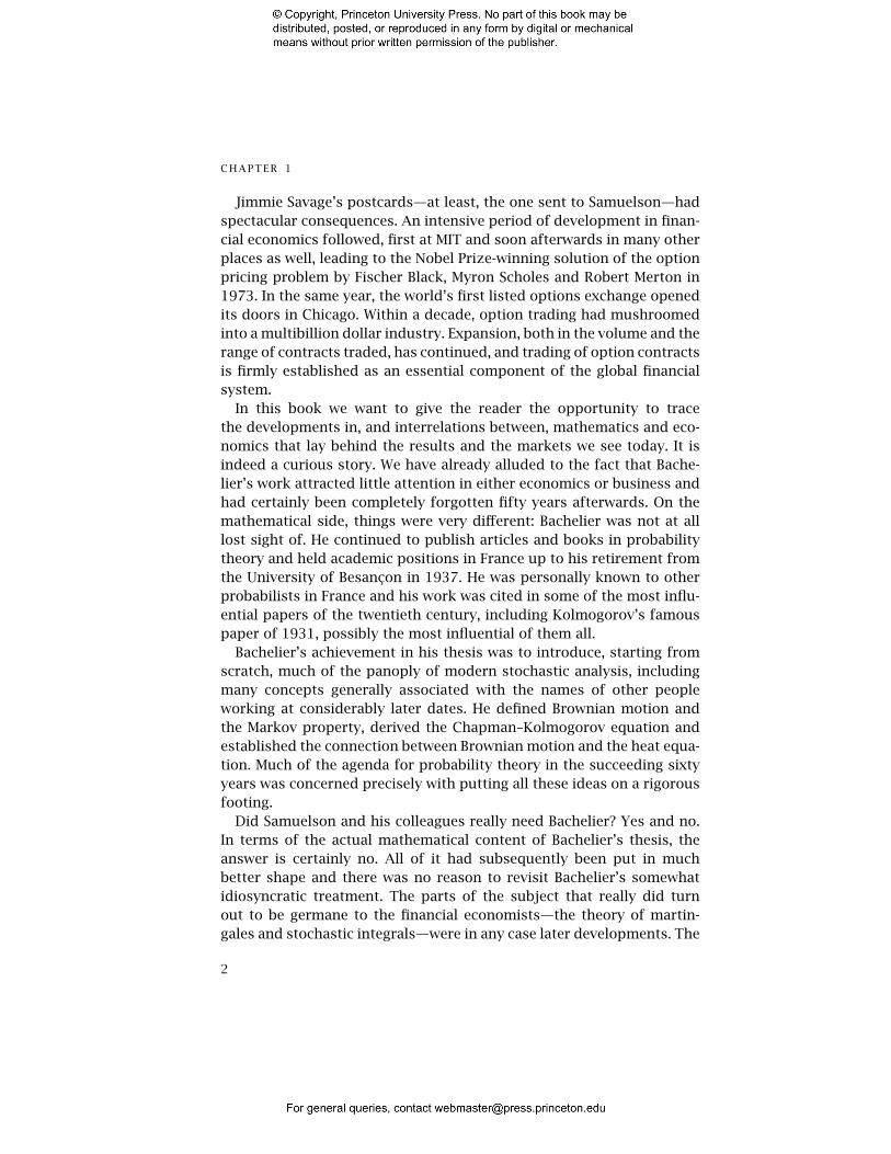
Figure 1.1. Returns from investing in asset (dashed line) and investing in call option (solid line) as functions of asset price at maturity date. Initial asset price is 100.

100 150500%

100%

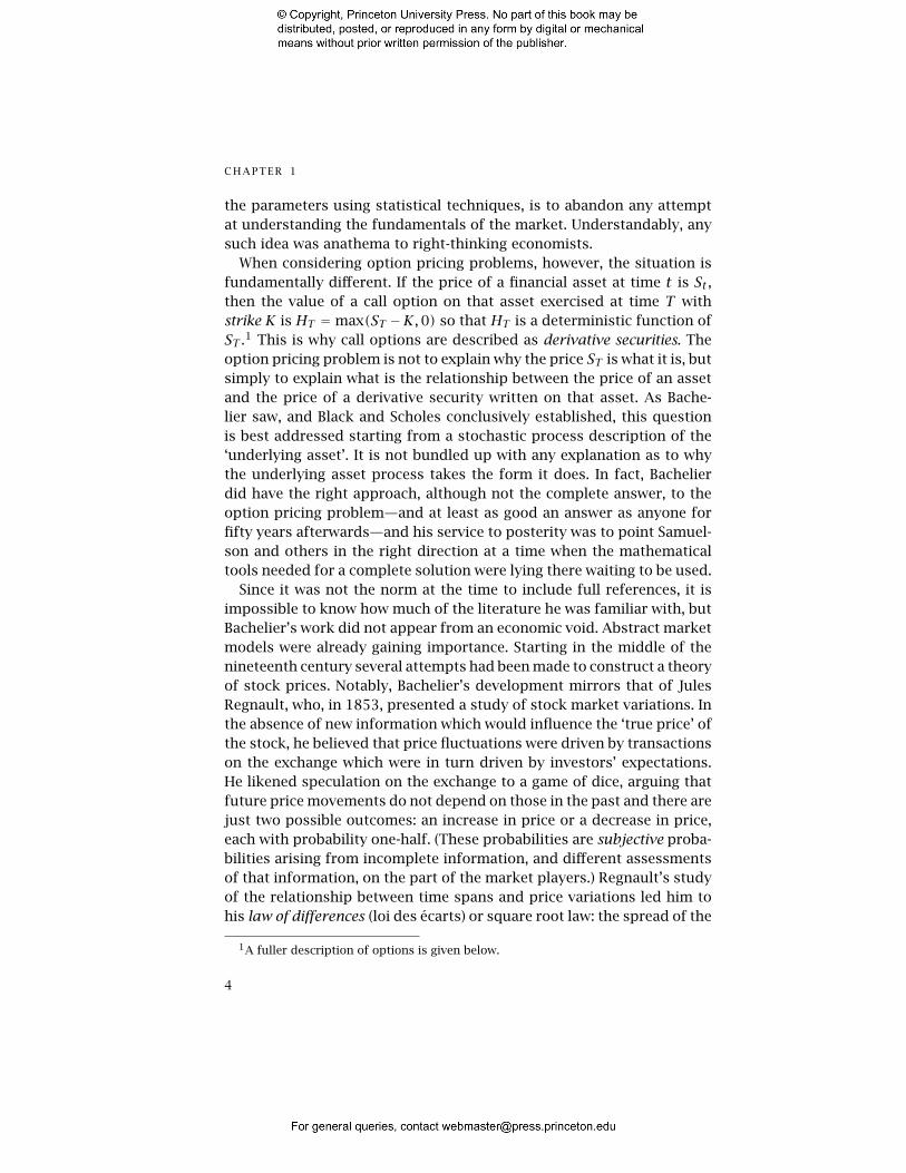
Figure 1.2. Returns from investing in option strategy with money-back guar­antee return (solid line) and simple investment strategy with money-back guar­antee.

the other hand if it rises by 20% then the option pays £2, a 100% return on the investment (as opposed to the 20% return gained by investing in the stock itself). The option investor is taking a massive risk—the risk of losing his entire investment—to back his view that the price will rise. For this reason option contracts have always had a slightly disreputable air about them, which continues to the present day. Lawsuits are regu­larly taken out by aggrieved parties claiming that the risks in option-like investments were not properly explained to them.

Figure 1.1 shows the return as a function of price for simple invest­ment and for investment in options. Viewed in this way, a ‘naked’ posi­tion in options does seem like playing with fire. Nonetheless, by mixing with other investments, the buyer of an option can take advantage of leveraged returns while limiting his downside loss liabilities. For exam­ple, investment products are sometimes offered that guarantee investors at least their ‘money back’ after, say, five years. Suppose the interest

7

C H A P T E R 1

rate for a five-year deposit is 4%. Then a deposit of £82.19 matures with a value of £100 in five years’ time. The investment company can offer the money-back guarantee by investing £82.19 of each £100 in this way and ‘playing the market’ with the remaining £17.81. Figure 1.2 shows the return as a function of underlying asset for investment in the asset itself or in options as described above. Arguably, the latter provides a more attractive return profile to investors: there is the possibility of a substantial gain and the downside is limited to interest lost by not just keeping the money in the bank.

A more benign, and economically far more important, use of options is in connection with hedging risks. Used in this way, an option is not a leveraged investment but, on the contrary, is expressly designed to offset risk. This effect is closely related to a simpler transaction, the forward contract. Suppose Alice in London wants to buy, off-plan, a flat on the Costa del Sol. The agreed price is €600,000, to be paid when the building is completed in one year’s time. This is equal to £400,000 at today’s exchange rate of €1.5 : £1. But of course Alice now has exchange rate risk: if the rate of exchange were to fall to 1.4 : 1, a not grossly improbable contingency, Alice’s bill rises by an unpleasant £28,571. She can protect herself against this in the following way. Let us say that Alice is able to borrow in England at an annual rate of 6%, and has a deposit account in Spain paying 2%. If she borrows £600,000/(1.5 × 1.02) £392,157,=converts it into euros and deposits this sum in the Spanish account, the value of the account in one year will be exactly the €600,000 she has agreed to pay. But meanwhile her negative balance in England will be £392,157 × 1.06 £415,686, so the effective exchange rate for the =transaction is 600,000/415,686 1.443, which is the rate she should = be allowing for when agreeing the price. But, in addition to protecting herself against a loss, Alice has also protected herself against a profit: if the foreign exchange rate were instead to move to 1.6, Alice would, in retrospect, have been better off sitting back and taking the profit of £25,000. What she wants is the best of both worlds: a fixed exchange rate X and the right to use either that rate or the market spot rate, whichever is the more favourable. This is the classic call option. By buying a call option, Alice is in effect insuring herself against the exchange rate falling below X, so she should pay an insurance premium for that. What that premium should be is the option pricing problem.

The options that Bachelier was concerned with were written on les rentes, perpetual French government bonds. City or state government bonds have a long history, intricately bound up with the need to raise

8

MATHEMATICS AND FINANCE

money to wage war and to pay reparations after defeat.5 In the earliest examples the buyer was given little choice in the matter, but in 1522 perpetual annuities called rentes were floated free of coercion, secured by the tax on wine. Under these contracts the state undertook to pay an annuity for an indefinite period. They did not repay the principal although they did reserve the right to redeem the contract at any time. It did not take the rentiers long to appreciate the benefits of having taxes imposed on their behalf and they soon offered additional loans. But rentes have a chequered history. Twice in the seventeenth century payments were simply suspended. Finance ministers disallowed rentes created by their predecessors and created new ones, there was no uni­formity in conditions and no clear record of the outstanding government obligation. Each war saw more issues so that, for example, between 1774 and 1789 the total government debt tripled. The bad credit of the rev­olutionary government led them to issue assignats, obligations suppos­edly backed by land seized from nobility and the church, which bore interest and were to be redeemed in five years. But the interest was reduced and then abolished and the assignats were issued in smaller and smaller denominations so that they eventually became no more than paper money which lost all value if they were not redeemed. Finally, in 1797, they were declared valueless. In the same year the two-thirds bankruptcy law was passed whereby only one-third of the interest on the national debt and one-third of pensions was paid in cash, with the balance in land warrants of little or no real value. All confidence in the system was lost.

It was Napoleon who reformed the French finances. Starting in 1797 he established a budget, increased taxes and forcibly refunded the national debt through an issue of 5% rentes. All valid loans and titles to rentes were recorded in the Grand Livre, the great book of public debt, which had been created in 1793, and France entered the modern era of uni­form rentes. To service the debt, Napoleon reestablished the caisse d’amortissement, which he deposited, in return for shares, in the Banque de France. This semi-private organization, created by a group of his sup­porters in 1800, was not only granted the monopoly on Parisian ban­knotes, it also managed the rentes.

The nineteenth century was a period of political turmoil in France, nonetheless there was a large growth in banking and increasingly orderly finance. The rentes recovered quickly from successive political crises

5For a more detailed history, see Homer and Sylla (2005).

9

C H A P T E R 1

and although the interest was progressively reduced during the course of the century, by 1900 they were very popular with French investors as a relatively secure investment. Once issued their prices fluctuated, but the rentes had a nominal value, typically Fr 100, and paid a fixed return usually between 3% and 5%. At the time when Bachelier wrote his thesis, the nominal value of the debt was 26 billion francs (Taqqu 2001) and there was very considerable trade in rentes on the Paris Bourse, where they could be sold for cash or as forwards or options.

In 1914 stock exchanges all over the world were forced to close and whilst this did not signal the death of the international bond market, the collapse of the French franc over the course of the century, losing 99% of its dollar value in the period 1900–1990, spelt the end of an era for the rentiers (Ferguson 2001).

Gambling Strategies and Martingales

In the introduction to his 1968 book Probability, Leo Breiman points out that probability theory as we know it today derives from two sources: the mathematics of measure theory on the one hand, and gambling on the other.6 Perhaps its unsavoury relationship with games of chance is at least partially responsible for the fact that probability took a long time to be regarded as a respectable branch of mathematics. The flavour is caught to perfection by William Makepeace Thackeray in Chapter 64 of Vanity Fair :

There is no town of any mark in Europe but it has its little colony of English raffs—men whose names Mr. Hemp the officer reads out period­ically at the Sheriffs’ Court—young gentlemen of very good family often, only that the latter disowns them; frequenters of billiard-rooms and estaminets, patrons of foreign races and gaming-tables. They people the debtors’ prisons—they drink and swagger—they fight and brawl— they run away without paying—they have duels with French and Ger­man officers—they cheat Mr. Spooney at écarté—they get the money and drive off to Baden in magnificent britzkas—they try their infalli­ble martingale and lurk about the tables with empty pockets, shabby bullies, penniless bucks…

The ‘infallible martingale’ is a strategy for making a sure profit on games such as roulette in which one makes a sequence of independent bets. The strategy is to stake £1 (on, say, a specific number in roulette)

6He credits Michel Loève and David Blackwell, respectively, for teaching him the two sides.

10

MATHEMATICS AND FINANCE

Figure 1.3. Harness with martingale.

and keep doubling the stake until that number wins. When it does, all previous losses and more are recouped and one leaves the table with a profit. It does not matter how unfavourable the odds are, only that a winning play comes up eventually. In his memoirs, Casanova recounts winning a fortune at the roulette table playing a martingale, only to lose it a few days later.

The word ‘martingale’ has several uses outside gambling. It can mean a strap attached to a fencer’s épée, or a strut under the bowsprit of a sailing boat, but the most common usage is equestrian: the martin­gale refers to the strap of a horse’s harness that connects the girth to the noseband and prevents the horse from throwing back its head (see Figure 1.3). Like the gambling strategy, it allows free movement in one direction while preventing movement in the other. The mathematician Paul Halmos once sent J. L. Doob, who did more than any other single mathematician to develop the mathematical theory of martingales, an equestrian martingale. Doob had no idea what it was or why he had been sent it (Snell 2005).

The martingale is not infallible, as the penniless bucks whose names Mr Hemp read out at the Sheriffs’ Court could attest. Nailing down why, in precise terms, had to await the development of the theory of martin­gales (in the mathematical sense) by Doob in the 1940s. The term was introduced into probability theory by Ville in 1939, who initiated its use to describe the fortune of a player in a fair game rather than the gam­bling strategy employed by that player. A martingale is then a stochastic processes Xt such that the expected value of the process at some future time, given its past history up to today, is equal to today’s value. We write this Xs E[Xt | Fs], t > s. Roulette is not a fair game: the player’s =fortune is a supermartingale, meaning that the expected future value is

11

C H A P T E R 1

less than today’s value, Xs � E[Xt | Fs]. One of Doob’s key results is the optional sampling theorem. A stopping time (or optional time in Doob’s parlance) is a random time whose occurrence by time t can be detected by observing the evolution of the process Xs for s � t. For example, the time of the first winning play in roulette is a stopping time. The optional sam­pling theorem shows in particular that if Xt is a bounded supermartin­gale (i.e. |Xt| � c for some constant c) and S, T are two stopping times such that S � T with probability 1, then XS � E[XT | FS], i.e. the super-martingale inequality continues to hold if fixed times s, t are replaced by stopping times S, T . For a bounded martingale, XS = E[XT | FS].

Now suppose that Xt is the player’s fortune when he plays the mar­tingale strategy at roulette and T is the time of the first winning play. Xt is a supermartingale since the odds are biased in favour of the bank. The conditions of the optional sampling theorem are not met since Xt is not bounded (losses double up until the first winning play occurs, but we do not know how long we have to wait for this). And indeed the con­clusion of the theorem does not hold either: by definition XT > X0, so E[XT ] > E[X0]. Suppose, however, that there is a house limit : the player has to stop if his accumulated losses ever reach some prescribed level K. The conditions of the optional sampling theorem are satisfied for the process7 Yt Xt∧R, the player’s fortune up to the point R where he is =obliged to quit, so E[XT∧R] � X0. But this inequality can only hold if there is a positive probability that R < T , that is, there must be a chance that the house limit is reached before the winning play occurs. Thus any house limit, however large, turns the ‘martingale’ into an unfavourable strategy in which the player may lose his shirt. Every house has a limit of some kind.

The martingale idea plays a big part in Bachelier’s analysis, although he does not define it in any formal way and, of course, the name itself did not come into mathematical currency for a further thirty-nine years. Bachelier’s dictum (perhaps inherited from Regnault) was (see p. 28) ‘L’espérance mathematique du spéculateur est nulle’ (‘the speculator’s expected return is zero’). The argument for this is based on market sym­metry: any trade has two parties, a buyer and a seller, and they must agree on a price. It follows that there cannot be any consistent bias in favour of one or the other, so today’s price must be equal to the expected value of the price at any date in the future: exactly the martingale prop­erty. In Bachelier’s day, the option premium was paid in the form of a

7t ∧ s denotes the lesser of s and t.

12

∑

∑ ∑

MATHEMATICS AND FINANCE

‘forfeit’ paid at the exercise time of the option, and only paid if it was not exercised. Bachelier’s main pricing formula is obtained by taking the price process as scaled Brownian motion and computing the value of the forfeit such that the whole transaction has zero value. Given Bachelier’s price model this answer is actually correct but not, as we shall see, for quite the reasons Bachelier thought it was.

Deciding when to quit a game is a very simple kind of gambling (or investment) strategy. A correct theory of option pricing requires consid­eration of more sophisticated strategies in which funds are switched between different traded assets in a quite complicated way. Suppose there are N traded assets8 with price processes St (St

(1), . . . , St(N) ). A=

trading strategy is an N-vector process θ with the interpretation that the ith component θt

(i) is the number of units of asset i held at time t. An obvious requirement is that θt must be non-anticipative, i.e. can depend only on market variables that have been observed up to time t. We say that θt is ‘Ft-adapted’, or just ‘adapted’, where Ft denotes the history of the market up to time t. We call θt a simple trading strategy on the time interval [0, T ] if there is a sequence of fixed or stopping times 0 τ0 < τ1 < < τm � T such that θt θτi for t ∈ [τi, τi+1), that = · · · =is, trades are executed only at a finite number of times τi. Let us write ηi θτi . The strategy is self-financing if ηi Sτi ηi Sτi , which = · +1 = +1 · +1

just says that the trade at time τi+1 only rearranges the investment port­folio, it does not change its total value. It is a matter of algebra to verify that the following equality holds for any simple self-financing strategy, ∫ T

θT ST − θ0 S0 θt dSt, (1.1)· · = 0

·

where the right-hand side denotes the sum suggested by the notation ∫ T N ∫ T

0 θt · dSt =

i 1 0 θt(i) dSt

(i)

=N { m−1 }

= i 1

ηi (Si )+k 0

ηik(S(i)+1 − S(i)) . (1.2)m τ − Sτim τk τk

= =

Equation (1.1) states that the change in portfolio value (on the left-hand side) is equal to the ‘gain from trade’ (on the right-hand side). We can use (1.1) as the definition of ‘self-financing’, a definition which will go

8In the classic Black–Scholes set-up, N 2 : S(1) St is the price of the asset on which rt

= t =the option is written and St

(2) e is a money-market account paying continuously com­=pounding interest at rate r .

13

C H A P T E R 1

beyond the case of simple strategies. Black–Scholes style option pricing is largely concerned with finding self-financing trading strategies θt such that the final portfolio value θT ST is equal to some pre-specified ran­·dom variable, to wit, the option exercise value. Invariably, this cannot be achieved using simple strategies and we have to consider more general strategies which are in some sense limits of simple ones. The process of constructing these strategies and defining the corresponding gains from trade is exactly the process of constructing stochastic integrals with respect to martingales and semimartingales which was begun by Itô in the 1940s and completed by Meyer and Dellacherie in the late 1970s. As Itô explains in the foreword to the volume of his selected papers pub­lished in 1986, he noticed that, starting from any given instant, a Marko­vian process would perform a time homogeneous differential process for the infinitesimal future. This led him to the notion of a stochastic dif­ferential equation governing the paths of the particle which could then be made mathematically rigorous by writing it in integral form, but this intuition requires that when defining the integral of a simple integrand, the integrand should be evaluated at the left-hand end point of the inter­val, as it is in equation (1.2) above. In equation (1.2) we arrived at this definition from the natural economic requirement that the investment must be decided on before subsequent price moves are revealed. Thus Itô–Meyer–Dellacherie stochastic integrals are exactly the ones required for economic applications.

In J. L. Doob’s obituary of William Feller in 1970 he writes:

Mathematicians could manipulate equations inspired by events and expectations long before these concepts were formalized mathemati­cally as measurable sets and integrals. But deeper and subtler inves­tigations had to wait until the blessing and curse of direct physical significance had been replaced by the bleak reliability of abstract math­ematics.

The deep and subtle mathematics that underlies today’s financial mar­kets is all-pervasive in engineering and the sciences. It has long since emerged from the wilderness of bleak reliability and is once again blessed and cursed.

And now to Bachelier. The next chapter is a translation of Louis Bache­lier’s thesis. We have endeavoured to reflect his written style. We have used two types of annotation: comment boxes to explain the financial contracts, and traditional footnotes for clarifications, corrections and historical comments. Bachelier’s own footnotes are unnumbered and in italics. The original thesis itself is reproduced in facsimile in Chapter 4.

14