Chapter The Risk and Term Structure of Interest Rateshicksian.cocolog-nifty.com/irregular_economist... · A bond’s term to maturity also affects its interest rate, and ... in Chapter

120

PREVIEW In our supply and demand analysis of interest-rate behavior in Chapter 5, we exam-ined the determination of just one interest rate. Yet we saw earlier that there are enor-mous numbers of bonds on which the interest rates can and do differ. In this chapter,we complete the interest-rate picture by examining the relationship of the variousinterest rates to one another. Understanding why they differ from bond to bond canhelp businesses, banks, insurance companies, and private investors decide whichbonds to purchase as investments and which ones to sell.

We first look at why bonds with the same term to maturity have different inter-est rates. The relationship among these interest rates is called the risk structure ofinterest rates, although risk, liquidity, and income tax rules all play a role in deter-mining the risk structure. A bond’s term to maturity also affects its interest rate, andthe relationship among interest rates on bonds with different terms to maturity iscalled the term structure of interest rates. In this chapter, we examine the sourcesand causes of fluctuations in interest rates relative to one another and look at a num-ber of theories that explain these fluctuations.

Risk Structure of Interest Rates

Figure 1 shows the yields to maturity for several categories of long-term bonds from1919 to 2002. It shows us two important features of interest-rate behavior for bondsof the same maturity: Interest rates on different categories of bonds differ from oneanother in any given year, and the spread (or difference) between the interest ratesvaries over time. The interest rates on municipal bonds, for example, are above thoseon U.S. government (Treasury) bonds in the late 1930s but lower thereafter. In addi-tion, the spread between the interest rates on Baa corporate bonds (riskier than Aaacorporate bonds) and U.S. government bonds is very large during the GreatDepression years 1930–1933, is smaller during the 1940s–1960s, and then widensagain afterwards. What factors are responsible for these phenomena?

One attribute of a bond that influences its interest rate is its risk of default, whichoccurs when the issuer of the bond is unable or unwilling to make interest paymentswhen promised or pay off the face value when the bond matures. A corporation suf-fering big losses, such as Chrysler Corporation did in the 1970s, might be more likely

Default Risk

Ch a p te r

The Risk and Term Structure

of Interest Rates6

to suspend interest payments on its bonds.1 The default risk on its bonds wouldtherefore be quite high. By contrast, U.S. Treasury bonds have usually been consid-ered to have no default risk because the federal government can always increase taxesto pay off its obligations. Bonds like these with no default risk are called default-freebonds. (However, during the budget negotiations in Congress in 1995 and 1996, theRepublicans threatened to let Treasury bonds default, and this had an impact on thebond market, as one application following this section indicates.) The spread betweenthe interest rates on bonds with default risk and default-free bonds, called the riskpremium, indicates how much additional interest people must earn in order to bewilling to hold that risky bond. Our supply and demand analysis of the bond marketin Chapter 5 can be used to explain why a bond with default risk always has a posi-tive risk premium and why the higher the default risk is, the larger the risk premiumwill be.

To examine the effect of default risk on interest rates, let us look at the supply anddemand diagrams for the default-free (U.S. Treasury) and corporate long-term bondmarkets in Figure 2. To make the diagrams somewhat easier to read, let’s assume thatinitially corporate bonds have the same default risk as U.S. Treasury bonds. In thiscase, these two bonds have the same attributes (identical risk and maturity); theirequilibrium prices and interest rates will initially be equal (P c

1 5 P T1 and i c

1 5 i T1 ),

and the risk premium on corporate bonds (i c1 2 i T

1 ) will be zero.

C H A P T E R 6 The Risk and Term Structure of Interest Rates 121

F I G U R E 1 Long-Term Bond Yields, 1919–2002

Sources: Board of Governors of the Federal Reserve System, Banking and Monetary Statistics, 1941–1970; Federal Reserve: www.federalreserve.gov/releases/h15/data/.

16

14

12

10

8

6

4

2

0

1950 1960 1970 1980 1990 2000

State and Local Government(Municipal)

U.S. GovernmentLong-Term Bonds

Corporate Baa Bonds

Annual Yield (%)

Corporate Aaa Bonds

194019301920

1Chrysler did not default on its loans in this period, but it would have were it not for a government bailout plan

intended to preserve jobs, which in effect provided Chrysler with funds that were used to pay off creditors.

www.federalreserve.gov/Releases/h15/update/

The Federal Reserve reports thereturns on different quality

bonds. Look at the bottom ofthe listing of interest rates forAAA and BBB rated bonds.

Study Guide Two exercises will help you gain a better understanding of the risk structure:

1. Put yourself in the shoes of an investor—see how your purchase decision wouldbe affected by changes in risk and liquidity.

2. Practice drawing the appropriate shifts in the supply and demand curves whenrisk and liquidity change. For example, see if you can draw the appropriate shiftsin the supply and demand curves when, in contrast to the examples in the text,a corporate bond has a decline in default risk or an improvement in its liquidity.

If the possibility of a default increases because a corporation begins to suffer largelosses, the default risk on corporate bonds will increase, and the expected return onthese bonds will decrease. In addition, the corporate bond’s return will be moreuncertain as well. The theory of asset demand predicts that because the expectedreturn on the corporate bond falls relative to the expected return on the default-freeTreasury bond while its relative riskiness rises, the corporate bond is less desirable(holding everything else equal), and demand for it will fall. The demand curve forcorporate bonds in panel (a) of Figure 2 then shifts to the left, from D c

1 to D c2.

At the same time, the expected return on default-free Treasury bonds increasesrelative to the expected return on corporate bonds, while their relative riskiness

122 P A R T I I Financial Markets

F I G U R E 2 Response to an Increase in Default Risk on Corporate Bonds

An increase in default risk on corporate bonds shifts the demand curve from D c1 to D c

2. Simultaneously, it shifts the demand curve forTreasury bonds from D T

1 to D T2. The equilibrium price for corporate bonds (left axis) falls from P c

1 to P c2, and the equilibrium interest rate

on corporate bonds (right axis) rises from i c1 to i c

2. In the Treasury market, the equilibrium bond price rises from P T1 to P T

2, and the equilib-rium interest rate falls from i T

1 to i T2. The brace indicates the difference between i c

2 and i T2, the risk premium on corporate bonds. (Note: P

and i increase in opposite directions. P on the left vertical axis increases as we go up the axis, while i on the right vertical axis increases aswe go down the axis.)

Quantity of Corporate Bonds Quantity of Treasury Bonds

Price of Bonds, P(P increases ↑)

Interest Rate, i(i increases )

↑

Interest Rate, i(i increases )

↑


(a) Corporate bond market (b) Default-free (U.S. Treasury) bond market

RiskPremium

P c2

P c1

S c

D c1D c

2

i c1

P T2

P T1

i c2

S T

D T1

DT2

i T1

i T2

i T2

declines. The Treasury bonds thus become more desirable, and demand rises, asshown in panel (b) by the rightward shift in the demand curve for these bonds fromD T

1 to D T2.

As we can see in Figure 2, the equilibrium price for corporate bonds (left axis)falls from P c

1 to P c2, and since the bond price is negatively related to the interest rate,

the equilibrium interest rate on corporate bonds (right axis) rises from i c1 to i c

2. At thesame time, however, the equilibrium price for the Treasury bonds rises from P T

1 to P T2,

and the equilibrium interest rate falls from i T1 to i T

2. The spread between the interestrates on corporate and default-free bonds—that is, the risk premium on corporatebonds—has risen from zero to i c

2 2 i T2. We can now conclude that a bond with

default risk will always have a positive risk premium, and an increase in its defaultrisk will raise the risk premium.

Because default risk is so important to the size of the risk premium, purchasersof bonds need to know whether a corporation is likely to default on its bonds. Twomajor investment advisory firms, Moody’s Investors Service and Standard and Poor’sCorporation, provide default risk information by rating the quality of corporate andmunicipal bonds in terms of the probability of default. The ratings and their descrip-tion are contained in Table 1. Bonds with relatively low risk of default are calledinvestment-grade securities and have a rating of Baa (or BBB) and above. Bonds with


Rating

Standard Examples of Corporations with

Moody’s and Poor’s Descriptions Bonds Outstanding in 2003

Aaa AAA Highest quality General Electric, Pfizer Inc.,

(lowest default risk) North Carolina State,

Mobil Oil

Aa AA High quality Wal-Mart, McDonald’s,

Credit Suisse First Boston

A A Upper medium grade Hewlett-Packard,

Anheuser-Busch,

Ford, Household Finance

Baa BBB Medium grade Motorola, Albertson’s, Pennzoil,

Weyerhaeuser Co.,

Tommy Hilfiger

Ba BB Lower medium grade Royal Caribbean, Levi Strauss

B B Speculative Rite Aid, Northwest Airlines Inc.,

Six Flags

Caa CCC, CC Poor (high default risk) Revlon, United Airlines

Ca C Highly speculative US Airways, Polaroid

C D Lowest grade Enron, Oakwood Homes

Table 1 Bond Ratings by Moody’s and Standard and Poor’s

ratings below Baa (or BBB) have higher default risk and have been aptly dubbedspeculative-grade or junk bonds. Because these bonds always have higher interestrates than investment-grade securities, they are also referred to as high-yield bonds.

Next let’s look back at Figure 1 and see if we can explain the relationship betweeninterest rates on corporate and U.S. Treasury bonds. Corporate bonds always havehigher interest rates than U.S. Treasury bonds because they always have some risk ofdefault, whereas U.S. Treasury bonds do not. Because Baa-rated corporate bonds havea greater default risk than the higher-rated Aaa bonds, their risk premium is greater,and the Baa rate therefore always exceeds the Aaa rate. We can use the same analysisto explain the huge jump in the risk premium on Baa corporate bond rates during theGreat Depression years 1930–1933 and the rise in the risk premium after 1970 (seeFigure 1). The depression period saw a very high rate of business failures and defaults.As we would expect, these factors led to a substantial increase in default risk for bondsissued by vulnerable corporations, and the risk premium for Baa bonds reachedunprecedentedly high levels. Since 1970, we have again seen higher levels of businessfailures and defaults, although they were still well below Great Depression levels.Again, as expected, default risks and risk premiums for corporate bonds rose, widen-ing the spread between interest rates on corporate bonds and Treasury bonds.


The Enron Bankruptcy and the Baa-Aaa SpreadApplication

In December 2001, the Enron Corporation, a firm specializing in trading in theenergy market, and once the seventh-largest corporation in the United States,was forced to declare bankruptcy after it became clear that it had used shadyaccounting to hide its financial problems. (The Enron bankruptcy, the largestever in the United States, will be discussed further in Chapter 8.) Because of thescale of the bankruptcy and the questions it raised about the quality of the infor-mation in accounting statements, the Enron collapse had a major impact on thecorporate bond market. Let’s see how our supply and demand analysis explainsthe behavior of the spread between interest rates on lower quality (Baa-rated) andhighest quality (Aaa-rated) corporate bonds in the aftermath of the Enron failure.

As a consequence of the Enron bankruptcy, many investors began todoubt the financial health of corporations with lower credit ratings such asBaa. The increase in default risk for Baa bonds made them less desirable atany given interest rate, decreased the quantity demanded, and shifted thedemand curve for Baa bonds to the left. As shown in panel (a) of Figure 2,the interest rate on Baa bonds should have risen, which is indeed what hap-pened. Interest rates on Baa bonds rose by 24 basis points (0.24 percentagepoints) from 7.81% in November 2001 to 8.05% in December 2001. But theincrease in the perceived default risk for Baa bonds after the Enron bank-ruptcy made the highest quality (Aaa) bonds relatively more attractive andshifted the demand curve for these securities to the right—an outcomedescribed by some analysts as a “flight to quality.” Just as our analysis predictsin Figure 2, interest rates on Aaa bonds fell by 20 basis points, from 6.97%in November to 6.77% in December. The overall outcome was that thespread between interest rates on Baa and Aaa bonds rose by 44 basis pointsfrom 0.84% before the bankruptcy to 1.28% afterward.

Another attribute of a bond that influences its interest rate is its liquidity. As welearned in Chapter 4, a liquid asset is one that can be quickly and cheaply convertedinto cash if the need arises. The more liquid an asset is, the more desirable it is (hold-ing everything else constant). U.S. Treasury bonds are the most liquid of all long-termbonds, because they are so widely traded that they are the easiest to sell quickly andthe cost of selling them is low. Corporate bonds are not as liquid, because fewer bondsfor any one corporation are traded; thus it can be costly to sell these bonds in anemergency, because it might be hard to find buyers quickly.

How does the reduced liquidity of the corporate bonds affect their interest ratesrelative to the interest rate on Treasury bonds? We can use supply and demand analy-sis with the same figure that was used to analyze the effect of default risk, Figure 2,to show that the lower liquidity of corporate bonds relative to Treasury bondsincreases the spread between the interest rates on these two bonds. Let us start theanalysis by assuming that initially corporate and Treasury bonds are equally liquidand all their other attributes are the same. As shown in Figure 2, their equilibriumprices and interest rates will initially be equal: P c

1 5 P T1 and i c

1 5 i T1. If the corporate

bond becomes less liquid than the Treasury bond because it is less widely traded, then(as the theory of asset demand indicates) its demand will fall, shifting its demandcurve from D c

1 to D c2 as in panel (a). The Treasury bond now becomes relatively more

liquid in comparison with the corporate bond, so its demand curve shifts rightwardfrom D T

1 to D T2 as in panel (b). The shifts in the curves in Figure 2 show that the price

of the less liquid corporate bond falls and its interest rate rises, while the price of themore liquid Treasury bond rises and its interest rate falls.

The result is that the spread between the interest rates on the two bond types hasrisen. Therefore, the differences between interest rates on corporate bonds andTreasury bonds (that is, the risk premiums) reflect not only the corporate bond’sdefault risk but its liquidity, too. This is why a risk premium is more accurately a “riskand liquidity premium,” but convention dictates that it is called a risk premium.

Returning to Figure 1, we are still left with one puzzle—the behavior of municipalbond rates. Municipal bonds are certainly not default-free: State and local govern-ments have defaulted on the municipal bonds they have issued in the past, particu-larly during the Great Depression and even more recently in the case of OrangeCounty, California, in 1994 (more on this in Chapter 13). Also, municipal bonds arenot as liquid as U.S. Treasury bonds.

Why is it, then, that these bonds have had lower interest rates than U.S. Treasurybonds for at least 40 years, as indicated in Figure 1? The explanation lies in the factthat interest payments on municipal bonds are exempt from federal income taxes, afactor that has the same effect on the demand for municipal bonds as an increase intheir expected return.

Let us imagine that you have a high enough income to put you in the 35% incometax bracket, where for every extra dollar of income you have to pay 35 cents to the gov-ernment. If you own a $1,000-face-value U.S. Treasury bond that sells for $1,000 andhas a coupon payment of $100, you get to keep only $65 of the payment after taxes.Although the bond has a 10% interest rate, you actually earn only 6.5% after taxes.

Suppose, however, that you put your savings into a $1,000-face-value municipalbond that sells for $1,000 and pays only $80 in coupon payments. Its interest rate isonly 8%, but because it is a tax-exempt security, you pay no taxes on the $80 couponpayment, so you earn 8% after taxes. Clearly, you earn more on the municipal bond

Income TaxConsiderations

Liquidity


after taxes, so you are willing to hold the riskier and less liquid municipal bond eventhough it has a lower interest rate than the U.S. Treasury bond. (This was not truebefore World War II, when the tax-exempt status of municipal bonds did not conveymuch of an advantage because income tax rates were extremely low.)

Another way of understanding why municipal bonds have lower interest rates thanTreasury bonds is to use the supply and demand analysis displayed in Figure 3. Weassume that municipal and Treasury bonds have identical attributes and so have thesame bond prices and interest rates as drawn in the figure: P m

1 5 P T1 and i m

1 5 i T1. Once

the municipal bonds are given a tax advantage that raises their after-tax expected returnrelative to Treasury bonds and makes them more desirable, demand for them rises, andtheir demand curve shifts to the right, from D m

1 to D m2. The result is that their equilib-

rium bond price rises from Pm1 to P m

2, and their equilibrium interest rate falls from i m1 to

i m2. By contrast, Treasury bonds have now become less desirable relative to municipal

bonds; demand for Treasury bonds decreases, and D T1 shifts to D T

2. The Treasury bondprice falls from P T

1 to P T2, and the interest rate rises from i T

1 to i T2. The resulting lower

interest rates for municipal bonds and higher interest rates for Treasury bonds explainswhy municipal bonds can have interest rates below those of Treasury bonds.2


F I G U R E 3 Interest Rates on Municipal and Treasury Bonds

When the municipal bond is given tax-free status, demand for the municipal bond shifts rightward from Dm1 to Dm

2 and demandfor the Treasury bond shifts leftward from DT

1 to DT2. The equilibrium price of the municipal bond (left axis) rises from Pm

1 toP m

2, so its interest rate (right axis) falls from im1 to im

2, while the equilibrium price of the Treasury bond falls from PT1 to PT

2 andits interest rate rises from iT1 to iT2. The result is that municipal bonds end up with lower interest rates than those on Treasurybonds. (Note: P and i increase in opposite directions. P on the left vertical axis increases as we go up the axis, while i on theright vertical axis increases as we go down the axis.)

Quantity of Treasury BondsQuantity of Municipal Bonds


Interest Rate, i(i increases )↑


(a) Market for municipal bonds (b) Market for Treasury bonds

Interest Rate, i(i increases )↑

P m1

P m2

S m

D m1

i m1

i m2

D m2

P T2

P T1

S T

DT1DT

2

i T1

i T2

2In contrast to corporate bonds, Treasury bonds are exempt from state and local income taxes. Using the analy-

sis in the text, you should be able to show that this feature of Treasury bonds provides an additional reason why

interest rates on corporate bonds are higher than those on Treasury bonds.

The risk structure of interest rates (the relationship among interest rates on bondswith the same maturity) is explained by three factors: default risk, liquidity, and theincome tax treatment of the bond’s interest payments. As a bond’s default riskincreases, the risk premium on that bond (the spread between its interest rate and theinterest rate on a default-free Treasury bond) rises. The greater liquidity of Treasurybonds also explains why their interest rates are lower than interest rates on less liquidbonds. If a bond has a favorable tax treatment, as do municipal bonds, whose inter-est payments are exempt from federal income taxes, its interest rate will be lower.

Summary

Term Structure of Interest Rates

We have seen how risk, liquidity, and tax considerations (collectively embedded in therisk structure) can influence interest rates. Another factor that influences the interestrate on a bond is its term to maturity: Bonds with identical risk, liquidity, and taxcharacteristics may have different interest rates because the time remaining to matu-rity is different. A plot of the yields on bonds with differing terms to maturity but thesame risk, liquidity, and tax considerations is called a yield curve, and it describes theterm structure of interest rates for particular types of bonds, such as governmentbonds. The “Following the Financial News” box shows several yield curves forTreasury securities that were published in the Wall Street Journal. Yield curves can beclassified as upward-sloping, flat, and downward-sloping (the last sort is oftenreferred to as an inverted yield curve). When yield curves slope upward, as in the“Following the Financial News” box, the long-term interest rates are above the short-term interest rates; when yield curves are flat, short- and long-term interest rates arethe same; and when yield curves are inverted, long-term interest rates are belowshort-term interest rates. Yield curves can also have more complicated shapes inwhich they first slope up and then down, or vice versa. Why do we usually see


Effects of the Bush Tax Cut on Bond Interest RatesApplication

The Bush tax cut passed in 2001 scheduled a reduction of the top income taxbracket from 39% to 35% over a ten-year period. What is the effect of thisincome tax decrease on interest rates in the municipal bond market relativeto those in the Treasury bond market?

Our supply and demand analysis provides the answer. A decreased incometax rate for rich people means that the after-tax expected return on tax-freemunicipal bonds relative to that on Treasury bonds is lower, because theinterest on Treasury bonds is now taxed at a lower rate. Because municipalbonds now become less desirable, their demand decreases, shifting thedemand curve to the left, which lowers their price and raises their interestrate. Conversely, the lower income tax rate makes Treasury bonds more desir-able; this change shifts their demand curve to the right, raises their price, andlowers their interest rates.

Our analysis thus shows that the Bush tax cut raises the interest rates onmunicipal bonds relative to interest rates on Treasury bonds.

upward slopes of the yield curve as in the “Following the Financial News” box butsometimes other shapes?

Besides explaining why yield curves take on different shapes at different times, agood theory of the term structure of interest rates must explain the following threeimportant empirical facts:

1. As we see in Figure 4, interest rates on bonds of different maturities movetogether over time.

2. When short-term interest rates are low, yield curves are more likely to have anupward slope; when short-term interest rates are high, yield curves are morelikely to slope downward and be inverted.

3. Yield curves almost always slope upward, as in the “Following the FinancialNews” box.

Three theories have been put forward to explain the term structure of interestrates; that is, the relationship among interest rates on bonds of different maturitiesreflected in yield curve patterns: (1) the expectations theory, (2) the segmented mar-kets theory, and (3) the liquidity premium theory, each of which is described in thefollowing sections. The expectations theory does a good job of explaining the first twofacts on our list, but not the third. The segmented markets theory can explain fact 3but not the other two facts, which are well explained by the expectations theory.Because each theory explains facts that the other cannot, a natural way to seek a bet-ter understanding of the term structure is to combine features of both theories, whichleads us to the liquidity premium theory, which can explain all three facts.

If the liquidity premium theory does a better job of explaining the facts and ishence the most widely accepted theory, why do we spend time discussing the othertwo theories? There are two reasons. First, the ideas in these two theories provide the


Following the Financial News

The Wall Street Journal publishes a daily plot of the yieldcurves for Treasury securities, an example of which ispresented here. It is typically found on page 2 of the“Money and Investing” section.

The numbers on the vertical axis indicate the interestrate for the Treasury security, with the maturity given bythe numbers on the horizontal axis. For example, theyield curve marked “Yesterday” indicates that the interestrate on the three-month Treasury bill yesterday was1.25%, while the one-year bill had an interest rate of1.35% and the ten-year bond had an interest rate of4.0%. As you can see, the yield curves in the plot have thetypical upward slope.

Source: Wall Street Journal, Wednesday, January 22, 2003, p. C2.

Yield Curves

www.ratecurve.com/yc2.html

Check out today’s yield curve.

Treasury Yield CurveYield to maturity of current bills,

notes and bonds.

Source: Reuters

11.0

2.0

3.0

4.0

5.0%

3 6 2 5 10 30mos. yrs. maturity

Yesterday

1 month ago

1 year ago

groundwork for the liquidity premium theory. Second, it is important to see howeconomists modify theories to improve them when they find that the predicted resultsare inconsistent with the empirical evidence.

The expectations theory of the term structure states the following commonsenseproposition: The interest rate on a long-term bond will equal an average of short-terminterest rates that people expect to occur over the life of the long-term bond. Forexample, if people expect that short-term interest rates will be 10% on average overthe coming five years, the expectations theory predicts that the interest rate on bondswith five years to maturity will be 10% too. If short-term interest rates were expectedto rise even higher after this five-year period so that the average short-term interestrate over the coming 20 years is 11%, then the interest rate on 20-year bonds wouldequal 11% and would be higher than the interest rate on five-year bonds. We can seethat the explanation provided by the expectations theory for why interest rates onbonds of different maturities differ is that short-term interest rates are expected tohave different values at future dates.

The key assumption behind this theory is that buyers of bonds do not preferbonds of one maturity over another, so they will not hold any quantity of a bond ifits expected return is less than that of another bond with a different maturity. Bondsthat have this characteristic are said to be perfect substitutes. What this means in prac-tice is that if bonds with different maturities are perfect substitutes, the expectedreturn on these bonds must be equal.

ExpectationsTheory


F I G U R E 4 Movements over Time of Interest Rates on U.S. Government Bonds with Different Maturities

Sources: Board of Governors of the Federal Reserve System, Banking and Monetary Statistics, 1941–1970; Federal Reserve: www.federalreserve.gov/releases/h15

/data.htm#top.

16

14

12

10

8

6

4

2

01950 1955 1960 1965 1970 1975 1980 1985 1990 1995 2000

20-Year BondAverages

Three-Month Bills(Short-Term)

Three-toFive-YearAverages

InterestRate (%)

To see how the assumption that bonds with different maturities are perfect sub-stitutes leads to the expectations theory, let us consider the following two investmentstrategies:

1. Purchase a one-year bond, and when it matures in one year, purchase anotherone-year bond.

2. Purchase a two-year bond and hold it until maturity.

Because both strategies must have the same expected return if people are holdingboth one- and two-year bonds, the interest rate on the two-year bond must equal theaverage of the two one-year interest rates. For example, let’s say that the current interestrate on the one-year bond is 9% and you expect the interest rate on the one-year bondnext year to be 11%. If you pursue the first strategy of buying the two one-year bonds,the expected return over the two years will average out to be (9% 1 11%)/2 5 10% peryear. You will be willing to hold both the one- and two-year bonds only if the expectedreturn per year of the two-year bond equals this. Therefore, the interest rate on the two-year bond must equal 10%, the average interest rate on the two one-year bonds.

We can make this argument more general. For an investment of $1, consider thechoice of holding, for two periods, a two-period bond or two one-period bonds.Using the definitions

it 5 today’s (time t) interest rate on a one-period bondi e

t11 5 interest rate on a one-period bond expected for next period (time t 1 1)i2t 5 today’s (time t) interest rate on the two-period bond

the expected return over the two periods from investing $1 in the two-period bondand holding it for the two periods can be calculated as:

(1 1 i2t )(1 1 i2t ) 2 1 5 1 1 2i2t 1 (i2t )2

2 1 = 2i2t 1 (i2t )2

After the second period, the $1 investment is worth (1 1 i2 t )(1 1 i2 t ). Subtractingthe $1 initial investment from this amount and dividing by the initial $1 investmentgives the rate of return calculated in the previous equation. Because (i2 t )

2 is extremelysmall—if i2 t 5 10% 5 0.10, then (i2 t )

25 0.01—we can simplify the expected return

for holding the two-period bond for the two periods to

2i2t

With the other strategy, in which one-period bonds are bought, the expectedreturn on the $1 investment over the two periods is:

(1 1 it)(1 1 i et11) 2 1 5 1 1 it 1 i e

t11 1 it(iet11) 2 1 5 it 1 i e

t 1 it(iet11)

This calculation is derived by recognizing that after the first period, the $1 investmentbecomes 1 1 it , and this is reinvested in the one-period bond for the next period,yielding an amount (1 1 it )(1 1 i e

t11). Then subtracting the $1 initial investmentfrom this amount and dividing by the initial investment of $1 gives the expectedreturn for the strategy of holding one-period bonds for the two periods. Becauseit(i

et11) is also extremely small—if it 5 i e

t11 5 0.10, then it(iet11) 5 0.01—we can sim-

plify this to:

it 1 i et11

Both bonds will be held only if these expected returns are equal; that is, when:

2i2t 5 it 1 i et11


Solving for i2t in terms of the one-period rates, we have:

(1)

which tells us that the two-period rate must equal the average of the two one-periodrates. Graphically, this can be shown as:

We can conduct the same steps for bonds with a longer maturity so that we can exam-ine the whole term structure of interest rates. Doing so, we will find that the interestrate of int on an n-period bond must equal:

(2)

Equation 2 states that the n-period interest rate equals the average of the one-period interest rates expected to occur over the n-period life of the bond. This is arestatement of the expectations theory in more precise terms.3

A simple numerical example might clarify what the expectations theory inEquation 2 is saying. If the one-year interest rate over the next five years is expectedto be 5, 6, 7, 8, and 9%, Equation 2 indicates that the interest rate on the two-yearbond would be:

while for the five-year bond it would be:

Doing a similar calculation for the one-, three-, and four-year interest rates, youshould be able to verify that the one- to five-year interest rates are 5.0, 5.5, 6.0, 6.5,and 7.0%, respectively. Thus we see that the rising trend in expected short-term inter-est rates produces an upward-sloping yield curve along which interest rates rise asmaturity lengthens.

The expectations theory is an elegant theory that provides an explanation of whythe term structure of interest rates (as represented by yield curves) changes at differ-ent times. When the yield curve is upward-sloping, the expectations theory suggeststhat short-term interest rates are expected to rise in the future, as we have seen in ournumerical example. In this situation, in which the long-term rate is currently abovethe short-term rate, the average of future short-term rates is expected to be higherthan the current short-term rate, which can occur only if short-term interest rates areexpected to rise. This is what we see in our numerical example. When the yield curveis inverted (slopes downward), the average of future short-term interest rates is

5% 1 6% 1 7% 1 8% 1 9%

55 7%

5% 1 6%

25 5.5%

in t 5

it 1 i et11 1 i e

t121 . . . 1 i et1(n21)

n

Today0

Year1

Year2

i t i et11

i 2t 5i t 1 i e

t11

2

i2t 5it 1 i e

t11

2


3The analysis here has been conducted for discount bonds. Formulas for interest rates on coupon bonds would

differ slightly from those used here, but would convey the same principle.

expected to be below the current short-term rate, implying that short-term interestrates are expected to fall, on average, in the future. Only when the yield curve is flatdoes the expectations theory suggest that short-term interest rates are not expected tochange, on average, in the future.

The expectations theory also explains fact 1 that interest rates on bonds with dif-ferent maturities move together over time. Historically, short-term interest rates havehad the characteristic that if they increase today, they will tend to be higher in thefuture. Hence a rise in short-term rates will raise people’s expectations of future short-term rates. Because long-term rates are the average of expected future short-termrates, a rise in short-term rates will also raise long-term rates, causing short- and long-term rates to move together.

The expectations theory also explains fact 2 that yield curves tend to have anupward slope when short-term interest rates are low and are inverted when short-term rates are high. When short-term rates are low, people generally expect them torise to some normal level in the future, and the average of future expected short-termrates is high relative to the current short-term rate. Therefore, long-term interest rateswill be substantially above current short-term rates, and the yield curve would thenhave an upward slope. Conversely, if short-term rates are high, people usually expectthem to come back down. Long-term rates would then drop below short-term ratesbecause the average of expected future short-term rates would be below current short-term rates and the yield curve would slope downward and become inverted.4

The expectations theory is an attractive theory because it provides a simple expla-nation of the behavior of the term structure, but unfortunately it has a major short-coming: It cannot explain fact 3, which says that yield curves usually slope upward.The typical upward slope of yield curves implies that short-term interest rates are usu-ally expected to rise in the future. In practice, short-term interest rates are just aslikely to fall as they are to rise, and so the expectations theory suggests that the typi-cal yield curve should be flat rather than upward-sloping.

As the name suggests, the segmented markets theory of the term structure sees mar-kets for different-maturity bonds as completely separate and segmented. The interestrate for each bond with a different maturity is then determined by the supply of anddemand for that bond with no effects from expected returns on other bonds withother maturities.

The key assumption in the segmented markets theory is that bonds of differentmaturities are not substitutes at all, so the expected return from holding a bond of onematurity has no effect on the demand for a bond of another maturity. This theory ofthe term structure is at the opposite extreme to the expectations theory, whichassumes that bonds of different maturities are perfect substitutes.

The argument for why bonds of different maturities are not substitutes is thatinvestors have strong preferences for bonds of one maturity but not for another, sothey will be concerned with the expected returns only for bonds of the maturity theyprefer. This might occur because they have a particular holding period in mind, and

SegmentedMarkets Theory


4The expectations theory explains another important fact about the relationship between short-term and long-term

interest rates. As you can see in Figure 4, short-term interest rates are more volatile than long-term rates. If inter-

est rates are mean-reverting—that is, if they tend to head back down after they are at unusually high levels or go

back up when they are at unusually low levels—then an average of these short-term rates must necessarily have

lower volatility than the short-term rates themselves. Because the expectations theory suggests that the long-term

rate will be an average of future short-term rates, it implies that the long-term rate will have lower volatility than

short-term rates.

if they match the maturity of the bond to the desired holding period, they can obtaina certain return with no risk at all.5 (We have seen in Chapter 4 that if the term tomaturity equals the holding period, the return is known for certain because it equalsthe yield exactly, and there is no interest-rate risk.) For example, people who have ashort holding period would prefer to hold short-term bonds. Conversely, if you wereputting funds away for your young child to go to college, your desired holding periodmight be much longer, and you would want to hold longer-term bonds.

In the segmented markets theory, differing yield curve patterns are accounted forby supply and demand differences associated with bonds of different maturities. If, asseems sensible, investors have short desired holding periods and generally preferbonds with shorter maturities that have less interest-rate risk, the segmented marketstheory can explain fact 3 that yield curves typically slope upward. Because in the typ-ical situation the demand for long-term bonds is relatively lower than that for short-term bonds, long-term bonds will have lower prices and higher interest rates, andhence the yield curve will typically slope upward.

Although the segmented markets theory can explain why yield curves usuallytend to slope upward, it has a major flaw in that it cannot explain facts 1 and 2.Because it views the market for bonds of different maturities as completely segmented,there is no reason for a rise in interest rates on a bond of one maturity to affect theinterest rate on a bond of another maturity. Therefore, it cannot explain why interestrates on bonds of different maturities tend to move together (fact 1). Second, becauseit is not clear how demand and supply for short- versus long-term bonds change withthe level of short-term interest rates, the theory cannot explain why yield curves tendto slope upward when short-term interest rates are low and to be inverted whenshort-term interest rates are high (fact 2).

Because each of our two theories explains empirical facts that the other cannot, alogical step is to combine the theories, which leads us to the liquidity premium theory.

The liquidity premium theory of the term structure states that the interest rate on along-term bond will equal an average of short-term interest rates expected to occurover the life of the long-term bond plus a liquidity premium (also referred to as a termpremium) that responds to supply and demand conditions for that bond.

The liquidity premium theory’s key assumption is that bonds of different maturi-ties are substitutes, which means that the expected return on one bond does influencethe expected return on a bond of a different maturity, but it allows investors to preferone bond maturity over another. In other words, bonds of different maturities areassumed to be substitutes but not perfect substitutes. Investors tend to prefer shorter-term bonds because these bonds bear less interest-rate risk. For these reasons,investors must be offered a positive liquidity premium to induce them to hold longer-term bonds. Such an outcome would modify the expectations theory by adding a pos-itive liquidity premium to the equation that describes the relationship between long-and short-term interest rates. The liquidity premium theory is thus written as:

(3)int 5it 1 i e

t111 i et12 1 . . . 1 i e

t1(n21)

n1 lnt

Liquidity Premium andPreferred HabitatTheories


5The statement that there is no uncertainty about the return if the term to maturity equals the holding period is

literally true only for a discount bond. For a coupon bond with a long holding period, there is some risk because

coupon payments must be reinvested before the bond matures. Our analysis here is thus being conducted for

discount bonds. However, the gist of the analysis remains the same for coupon bonds because the amount of this

risk from reinvestment is small when coupon bonds have the same term to maturity as the holding period.

where lnt 5 the liquidity (term) premium for the n-period bond at time t, which isalways positive and rises with the term to maturity of the bond, n.

Closely related to the liquidity premium theory is the preferred habitat theory,which takes a somewhat less direct approach to modifying the expectations hypothe-sis but comes up with a similar conclusion. It assumes that investors have a prefer-ence for bonds of one maturity over another, a particular bond maturity (preferredhabitat) in which they prefer to invest. Because they prefer bonds of one maturity overanother they will be willing to buy bonds that do not have the preferred maturity onlyif they earn a somewhat higher expected return. Because investors are likely to preferthe habitat of short-term bonds over that of longer-term bonds, they are willing tohold long-term bonds only if they have higher expected returns. This reasoning leadsto the same Equation 3 implied by the liquidity premium theory with a term premiumthat typically rises with maturity.

The relationship between the expectations theory and the liquidity premiums andpreferred habitat theories is shown in Figure 5. There we see that because the liquid-ity premium is always positive and typically grows as the term to maturity increases,the yield curve implied by the liquidity premium theory is always above the yieldcurve implied by the expectations theory and generally has a steeper slope.

A simple numerical example similar to the one we used for the expectationshypothesis further clarifies what the liquidity premium and preferred habitat theoriesin Equation 3 are saying. Again suppose that the one-year interest rate over the nextfive years is expected to be 5, 6, 7, 8, and 9%, while investors’ preferences for hold-ing short-term bonds means that the liquidity premiums for one- to five-year bondsare 0, 0.25, 0.5, 0.75, and 1.0%, respectively. Equation 3 then indicates that the inter-est rate on the two-year bond would be:

5% 1 6%

21 0.25% 5 5.75%


http://stockcharts.com/charts/YieldCurve.html

This site lets you look at thedynamic yield curve at anypoint in time since 1995.

F I G U R E 5 The Relationship

Between the Liquidity Premium

(Preferred Habitat) and Expectations

Theory

Because the liquidity premium isalways positive and grows as theterm to maturity increases, theyield curve implied by the liquid-ity premium and preferred habitattheories is always above the yieldcurve implied by the expectationstheory and has a steeper slope.Note that the yield curve impliedby the expectations theory isdrawn under the scenario ofunchanging future one-year inter-est rates.

302520151050

Years to Maturity, n

InterestRate, i

nt

Expectations TheoryYield Curve

Liquidity Premium, l

nt

Liquidity Premium (Preferred Habitat) TheoryYield Curve

while for the five-year bond it would be:

Doing a similar calculation for the one-, three-, and four-year interest rates, youshould be able to verify that the one- to five-year interest rates are 5.0, 5.75, 6.5, 7.25,and 8.0%, respectively. Comparing these findings with those for the expectations the-ory, we see that the liquidity premium and preferred habitat theories produce yieldcurves that slope more steeply upward because of investors’ preferences for short-term bonds.

Let’s see if the liquidity premium and preferred habitat theories are consistentwith all three empirical facts we have discussed. They explain fact 1 that interest rateson different-maturity bonds move together over time: A rise in short-term interestrates indicates that short-term interest rates will, on average, be higher in the future,and the first term in Equation 3 then implies that long-term interest rates will risealong with them.

They also explain why yield curves tend to have an especially steep upwardslope when short-term interest rates are low and to be inverted when short-termrates are high (fact 2). Because investors generally expect short-term interest ratesto rise to some normal level when they are low, the average of future expected short-term rates will be high relative to the current short-term rate. With the additionalboost of a positive liquidity premium, long-term interest rates will be substantiallyabove current short-term rates, and the yield curve would then have a steep upwardslope. Conversely, if short-term rates are high, people usually expect them to comeback down. Long-term rates would then drop below short-term rates because theaverage of expected future short-term rates would be so far below current short-term rates that despite positive liquidity premiums, the yield curve would slopedownward.

The liquidity premium and preferred habitat theories explain fact 3 that yieldcurves typically slope upward by recognizing that the liquidity premium rises with abond’s maturity because of investors’ preferences for short-term bonds. Even if short-term interest rates are expected to stay the same on average in the future, long-terminterest rates will be above short-term interest rates, and yield curves will typicallyslope upward.

How can the liquidity premium and preferred habitat theories explain the occa-sional appearance of inverted yield curves if the liquidity premium is positive? It mustbe that at times short-term interest rates are expected to fall so much in the future thatthe average of the expected short-term rates is well below the current short-term rate.Even when the positive liquidity premium is added to this average, the resulting long-term rate will still be below the current short-term interest rate.

As our discussion indicates, a particularly attractive feature of the liquidity pre-mium and preferred habitat theories is that they tell you what the market is predict-ing about future short-term interest rates just from the slope of the yield curve. Asteeply rising yield curve, as in panel (a) of Figure 6, indicates that short-term inter-est rates are expected to rise in the future. A moderately steep yield curve, as in panel(b), indicates that short-term interest rates are not expected to rise or fall much in thefuture. A flat yield curve, as in panel (c), indicates that short-term rates are expectedto fall moderately in the future. Finally, an inverted yield curve, as in panel (d), indi-cates that short-term interest rates are expected to fall sharply in the future.

5% 1 6% 1 7% 1 8% 1 9%

51 1% 5 8%


In the 1980s, researchers examining the term structure of interest rates questionedwhether the slope of the yield curve provides information about movements of futureshort-term interest rates.6 They found that the spread between long- and short-terminterest rates does not always help predict future short-term interest rates, a findingthat may stem from substantial fluctuations in the liquidity (term) premium for long-term bonds. More recent research using more discriminating tests now favors a dif-ferent view. It shows that the term structure contains quite a bit of information for thevery short run (over the next several months) and the long run (over several years)

Evidence on theTerm Structure


6Robert J. Shiller, John Y. Campbell, and Kermit L. Schoenholtz, “Forward Rates and Future Policy: Interpreting

the Term Structure of Interest Rates,” Brookings Papers on Economic Activity 1 (1983): 173–217; N. Gregory

Mankiw and Lawrence H. Summers, “Do Long-Term Interest Rates Overreact to Short-Term Interest Rates?”

Brookings Papers on Economic Activity 1 (1984): 223–242.

F I G U R E 6 Yield Curves and the Market’s Expectations of Future Short-Term Interest Rates According to the Liquidity Premium Theory

Term to Maturity

Term to Maturity

Term to Maturity

Term to Maturity

(a) Future short-term interest rates

expected to rise

(b) Future short-term interest rates

expected to stay the same

(c) Future short-term interest rates

expected to fall moderately

(d) Future short-term interest rates

expected to fall sharply

Yield toMaturity

Yield toMaturity

Yield toMaturity

Yield toMaturity

but is unreliable at predicting movements in interest rates over the intermediate term(the time in between).7

The liquidity premium and preferred habitat theories are the most widely acceptedtheories of the term structure of interest rates because they explain the major empir-ical facts about the term structure so well. They combine the features of both theexpectations theory and the segmented markets theory by asserting that a long-terminterest rate will be the sum of a liquidity (term) premium and the average of theshort-term interest rates that are expected to occur over the life of the bond.

The liquidity premium and preferred habitat theories explain the following facts:(1) Interest rates on bonds of different maturities tend to move together over time, (2)yield curves usually slope upward, and (3) when short-term interest rates are low,yield curves are more likely to have a steep upward slope, whereas when short-terminterest rates are high, yield curves are more likely to be inverted.

The theories also help us predict the movement of short-term interest rates in thefuture. A steep upward slope of the yield curve means that short-term rates are expectedto rise, a mild upward slope means that short-term rates are expected to remain thesame, a flat slope means that short-term rates are expected to fall moderately, and aninverted yield curve means that short-term rates are expected to fall sharply.

Summary


7Eugene Fama, “The Information in the Term Structure,” Journal of Financial Economics 13 (1984): 509–528;

Eugene Fama and Robert Bliss, “The Information in Long-Maturity Forward Rates,” American Economic Review 77

(1987): 680–692; John Y. Campbell and Robert J. Shiller, “Cointegration and Tests of the Present Value Models,”

Journal of Political Economy 95 (1987): 1062–1088; John Y. Campbell and Robert J. Shiller, “Yield Spreads and

Interest Rate Movements: A Bird’s Eye View,” Review of Economic Studies 58 (1991): 495–514.

Interpreting Yield Curves, 1980–2003Application

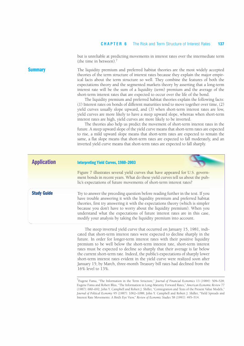
Figure 7 illustrates several yield curves that have appeared for U.S. govern-ment bonds in recent years. What do these yield curves tell us about the pub-lic’s expectations of future movements of short-term interest rates?

Study Guide Try to answer the preceding question before reading further in the text. If youhave trouble answering it with the liquidity premium and preferred habitattheories, first try answering it with the expectations theory (which is simplerbecause you don’t have to worry about the liquidity premium). When youunderstand what the expectations of future interest rates are in this case,modify your analysis by taking the liquidity premium into account.

The steep inverted yield curve that occurred on January 15, 1981, indi-cated that short-term interest rates were expected to decline sharply in thefuture. In order for longer-term interest rates with their positive liquiditypremium to be well below the short-term interest rate, short-term interestrates must be expected to decline so sharply that their average is far belowthe current short-term rate. Indeed, the public’s expectations of sharply lowershort-term interest rates evident in the yield curve were realized soon afterJanuary 15; by March, three-month Treasury bill rates had declined from the16% level to 13%.


The steep upward-sloping yield curves on March 28, 1985, and January23, 2003, indicated that short-term interest rates would climb in the future.The long-term interest rate is above the short-term interest rate when short-term interest rates are expected to rise because their average plus the liquid-ity premium will be above the current short-term rate. The moderatelyupward-sloping yield curves on May 16, 1980, and March 3, 1997, indicatedthat short-term interest rates were expected neither to rise nor to fall in thenear future. In this case, their average remains the same as the current short-term rate, and the positive liquidity premium for longer-term bonds explainsthe moderate upward slope of the yield curve.

F I G U R E 7 Yield Curves for U.S. Government Bonds

Sources: Federal Reserve Bank of St. Louis; U.S. Financial Data, various issues; Wall Street Journal, various dates.

1 2 3 4 5 5 10 15 20

6

8

10

12

14

16

Terms to Maturity (Years)

Interest Rate (%)

May 16, 1980

March 28, 1985

January 15, 1981

March 3, 1997

0

4

2

January 23, 2003

Summary

1. Bonds with the same maturity will have different

interest rates because of three factors: default risk,

liquidity, and tax considerations. The greater a bond’s

default risk, the higher its interest rate relative to other

bonds; the greater a bond’s liquidity, the lower its

interest rate; and bonds with tax-exempt status will

have lower interest rates than they otherwise would.

The relationship among interest rates on bonds with the

same maturity that arise because of these three factors is

known as the risk structure of interest rates.


2. Four theories of the term structure provide

explanations of how interest rates on bonds with

different terms to maturity are related. The expectations

theory views long-term interest rates as equaling the

average of future short-term interest rates expected to

occur over the life of the bond; by contrast, the

segmented markets theory treats the determination of

interest rates for each bond’s maturity as the outcome of

supply and demand in that market only. Neither of

these theories by itself can explain the fact that interest

rates on bonds of different maturities move together

over time and that yield curves usually slope upward.

3. The liquidity premium and preferred habitat theories

combine the features of the other two theories, and by

so doing are able to explain the facts just mentioned.

They view long-term interest rates as equaling the

average of future short-term interest rates expected to

occur over the life of the bond plus a liquidity

premium. These theories allow us to infer the market’s

expectations about the movement of future short-term

interest rates from the yield curve. A steeply upward-

sloping curve indicates that future short-term rates are

expected to rise, a mildly upward-sloping curve

indicates that short-term rates are expected to stay the

same, a flat curve indicates that short-term rates are

expected to decline slightly, and an inverted yield curve

indicates that a substantial decline in short-term rates is

expected in the future.

Key Terms

default, p. 120

default-free bonds, p. 121

expectations theory, p. 129

inverted yield curve, p. 127

junk bonds, p. 124

liquidity premium theory, p. 133

preferred habitat theory, p. 134

risk premium, p. 121

risk structure of interest rates, p. 120

segmented markets theory, p. 132

term structure of interest rates, p. 120

yield curve, p. 127

Questions and Problems

Questions marked with an asterisk are answered at the end

of the book in an appendix, “Answers to Selected Questions

and Problems.”

1. Which should have the higher risk premium on its

interest rates, a corporate bond with a Moody’s Baa

rating or a corporate bond with a C rating? Why?

*2. Why do U.S. Treasury bills have lower interest rates

than large-denomination negotiable bank CDs?

3. Risk premiums on corporate bonds are usually anticycli-

cal; that is, they decrease during business cycle expan-

sions and increase during recessions. Why is this so?

*4. “If bonds of different maturities are close substitutes, their

interest rates are more likely to move together.” Is this

statement true, false, or uncertain? Explain your answer.

5. If yield curves, on average, were flat, what would this

say about the liquidity (term) premiums in the term

structure? Would you be more or less willing to accept

the expectations theory?

*6. Assuming that the expectations theory is the correct

theory of the term structure, calculate the interest

rates in the term structure for maturities of one to five

years, and plot the resulting yield curves for the fol-

lowing series of one-year interest rates over the next

five years:

(a) 5%, 7%, 7%, 7%, 7%

(b) 5%, 4%, 4%, 4%, 4%

How would your yield curves change if people pre-

ferred shorter-term bonds over longer-term bonds?

7. Assuming that the expectations theory is the correct

theory of the term structure, calculate the interest rates

in the term structure for maturities of one to five years,

and plot the resulting yield curves for the following

path of one-year interest rates over the next five years:

(a) 5%, 6%, 7%, 6%, 5%

(b) 5%, 4%, 3%, 4%, 5%

How would your yield curves change if people pre-

ferred shorter-term bonds over longer-term bonds?

QUIZ

*8. If a yield curve looks like the one shown in figure (a)

in this section, what is the market predicting about

the movement of future short-term interest rates?

What might the yield curve indicate about the mar-

ket’s predictions about the inflation rate in the future?

9. If a yield curve looks like the one shown in (b), what

is the market predicting about the movement of future

short-term interest rates? What might the yield curve

indicate about the market’s predictions about the infla-

tion rate in the future?

*10. What effect would reducing income tax rates have on

the interest rates of municipal bonds? Would interest

rates of Treasury securities be affected, and if so, how?

Using Economic Analysis to Predict the Future

11. Predict what will happen to interest rates on a

corporation’s bonds if the federal government guaran-

tees today that it will pay creditors if the corporation

goes bankrupt in the future. What will happen to the

interest rates on Treasury securities?

*12. Predict what would happen to the risk premiums on

corporate bonds if brokerage commissions were low-

ered in the corporate bond market.

13. If the income tax exemption on municipal bonds were

abolished, what would happen to the interest rates on

these bonds? What effect would the change have on

interest rates on U.S. Treasury securities?

*14. If the yield curve suddenly becomes steeper, how

would you revise your predictions of interest rates in

the future?

15. If expectations of future short-term interest rates sud-

denly fall, what would happen to the slope of the

yield curve?


Web Exercises

1. The amount of additional interest investors receive

due to the various premiums changes over time.

Sometimes the risk premiums are much larger than at

other times. For example, the default risk premium

was very small in the late 1990s when the economy

was so healthy business failures were rare. This risk

premium increases during recessions.

Go to www.federalreserve.gov/releases/releases/h15

(historical data) and find the interest rate listings for

AAA and Baa rated bonds at three points in time, the

most recent, June 1, 1995, and June 1, 1992. Prepare

a graph that shows these three time periods (see

Figure 1 for an example). Are the risk premiums sta-

ble or do they change over time?

2. Figure 7 shows a number of yield curves at various

points in time. Go to www.bloomberg.com, and click

on “Markets” at the top of the page. Find the Treasury

yield curve. Does the current yield curve fall above or

below the most recent one listed in Figure 7? Is the

current yield curve flatter or steeper than the most

recent one reported in Figure 7?

3. Investment companies attempt to explain to investors

the nature of the risk the investor incurs when buying

shares in their mutual funds. For example, Vanguard

carefully explains interest rate risk and offers alterna-

tive funds with different interest rate risks. Go to

http://flagship5.vanguard.com/VGApp/hnw

/FundsStocksOverview.

a. Select the bond fund you would recommend to an

investor who has very low tolerance for risk and a

short investment horizon. Justify your answer.

b. Select the bond fund you would recommend to an

investor who has very high tolerance for risk and a

long investment horizon. Justify your answer.

Yield toMaturity

Term to Maturity(a)

Yield toMaturity

Term to Maturity(b)

Documents

Chapter The Risk and Term Structure of Interest Rateshicksian.cocolog-nifty.com/irregular_economist... · A bond’s term to maturity also affects its interest rate, and ... in Chapter