CHAPTER THEORIES OF STRESS AND STRAIN

CHAPTER 2 THEORIES OF STRESS AND STRAIN

I In Chapter 1, we presented general concepts and definitions that are fundamen-

tal to many of the topics discussed in this book. In this chapter, we develop theories of stress and strain that are essential for the analysis of a structural or mechanical system subjected to loads. The relations developed are used throughout the remainder of the book.

2.1 DEFINITION OF STRESS AT A POINT

Consider a general body subjected to forces acting on its surface (Figure 2.1). Pass a ficti- tious plane Q through the body, cutting the body along surface A (Figure 2.2). Designate one side of plane Q as positive and the other side as negative. The portion of the body on the positive side of Q exerts a force on the portion of the body on the negative side. This force is transmitted through the plane Q by direct contact of the parts of the body on the two sides of Q. Let the force that is transmitted through an incremental area AA of A by the part on the positive side of Q be denoted by AF. In accordance with Newton’s third law, the portion of the body on the negative side of Q transmits through area AA a force -AF.

The force A F may be resolved into components AFN and AFs, along unit normal N and unit tangent S, respectively, to the plane Q. The force AF, is called the normal force

FIGURE 2.1 A general loaded body cut by plane 0.

25

26 CHAPTER 2 THEORIES OF STRESS AND STRAIN

FIGURE 2.2 Force transmitted through incremental area of cut body.

on area AA and AFs is called the shear force on AA. The forces AF, AFN, and AFs depend on the location of area AA and the orientation of plane Q. The magnitudes of the average forces per unit area are AFIAA, AFNJAA, and AFs/AA. These ratios are called the average stress, average normal stress, and average shear stress, respectively, acting on area AA. The concept of stress at a point is obtained by letting AA become an infinitesimal. Then the forces AF, AFN, and AFs approach zero, but usually the ratios AFJAA, AFN/AA, and AFsIAA approach limits different from zero. The limiting ratio of AFIAA as AA goes to zero defines the stress vector u. Thus, the stress vector Q is given by

A F u = lim - A A + O M

The stress vector Q (also called the traction vector) always lies along the limiting direction of the force vector AF, which in general is neither normal nor tangent to the plane Q.

Similarly, the limiting ratios of AFNJAA and AFs/AA define the normal stress vector u, and the shear stress vector us that act at a point in the plane Q. These stress vectors are defined by the relations

AFS us = lim - AFN uN = lim - A A + O M A A + O

The unit vectors associated with uN and us are normal and tangent, respectively, to the plane Q.

2.2 STRESS NOTATION

Consider now a free-body diagram of a box-shaped volume element at a point 0 in a member, with sides parallel to the (x, y, z) axes (Figure 2.3). For simplicity, we show the volume element with one corner at point 0 and assume that the stress components are uniform (constant) throughout the volume element. The surface forces are given by the product of the stress components (Figure 2.3) and the areas' on which they act.

'You must remember to multiply each stress component by an appropriate area before applying equations of force equilibrium. For example, 0, must be multiplied by the area dy dz.

2.2 STRESS NOTATION 27

+ d x 4

FIGURE 2.3 Stress components at a point in loaded body.

FIGURE 2.4 Body forces.

Body forces? given by the product of the components (Bx, By, B,) and the volume of the element (product of the three infinitesimal lengths of the sides of the element), are higher-order terms and are not shown on the free-body diagram in Figure 2.3.

Consider the two faces perpendicular to the x axis. The face from which the positive x axis is extended is taken to be the positive face; the other face perpendicular to the x axis is taken to be the negative face. The stress components o,, oxy, and ox, acting on the positive face are taken to be in the positive sense as shown when they are directed in the positive x, y, and z directions. By Newton’s third law, the positive stress components o,, oxy, and o,, shown acting on the negative face in Figure 2.3 are in the negative (x, y, z) directions, respectively. In effect, a positive stress component o, exerts a tension (pull) parallel to the x axis. Equivalent sign conventions hold for the planes perpendicular to the y and z axes. Hence, associated with the concept of the state of stress at a point 0, nine components of stress exist:

In the next section we show that the nine stress components may be reduced to six for most practical problems.

’We use the notation B or (Bx, By , B,) for body force per unit volume, where B stands for body and subscripts (x, y, z) denote components in the (x. y, z ) directions, respectively, of the rectangular coordinate system (x, y, z ) (see Figure 2.4).


2.3 SYMMETRY OF THE STRESS ARRAY AND STRESS ON AN ARBITRARILY ORIENTED PLANE

2.3.1 Symmetry of Stress Components

The nine stress components relative to rectangular coordinate axes (x, y , z ) may be tabu- lated in array form as follows:

(2.3)

where T symbolically represents the stress array called the stress tensor. In this array, the stress components in the first, second, and third rows act on planes perpendicular to the (x, y, z ) axes, respectively.

Seemingly, nine stress components are required to describe the state of stress at a point in a member. However, if the only forces that act on the free body in Figure 2.3 are surface forces and body forces, we can demonstrate from the equilibrium of the volume element in Figure 2.3 that the three pairs of the shear stresses are equal. Summation of moments leads to the result

Thus, with Eq. 2.4, Eq. 2.3 may be written in the symmetric form

r 1

Hence, for this type of stress theory, only six components of stress are required to describe the state of stress at a point in a member.

Although we do not consider body couples or surface couples in this book (instead see Boresi and Chong, 2000), it is possible for them to be acting on the free body in Figure 2.3. This means that Eqs. 2.4 are no longer true and that nine stress components are required to represent the unsymmetrical state of stress.

The stress notation just described is widely used in engineering practice. It is the notation used in this book3 (see row I of Table 2.1). Two other frequently used symmetric stress notations are also listed in Table 2.1. The symbolism indicated in row I11 is employed where index notation is used (Boresi and Chong, 2000).

TABLE 2.1 Stress Notations (Symmetric Stress Components)

I 0 x x 0 Y Y 022 0 x y = 0 y x 0 x 2 = 0zx =yz = 0 z y

ll O X 0 2 zxy = zyx 7x2 = zzx zyz = Tzy

111 0 1 1 022 033 O12 = O21 013 = 4 1 023 = 032

3Equivalent notations are used for other orthogonal coordinate systems (see Section 2.5).

2.3 SYMMETRY OF THE STRESS ARRAY AND STRESS ON AN ARBITRARILY ORIENTED PLANE 29

2.3.2 Stresses Acting on Arbitrary Planes

The stress vectors a,, uy, and a, on planes that are perpendicular, respectively, to the x, y, and z axes are

ax = oXxi + oxy j + oxzk

a, = Q i + o,, j + oyzk uz = a,$ + a,, j + ozzk

Y X

where i, j, and k are unit vectors relative to the (x, y, z ) axes (see Figure 2.5 for u,).

ume element into a tetrahedron (Figure 2.6). The unit normal vector to plane P is Now consider the stress vector up on an arbitrary oblique plane P that cuts the vol-

N = l i + m j + n k (2.7)

where (I, m, n) are the direction cosines of unit vector N. Therefore, vectorial summation offorces acting on the tetrahedral element OABC yields the following (note that the ratios of areas OBC, OAC, OBA to area ABC are equal to I , m, and n, respectively):

up = l u x + m u y + n u , (2.8)

Also, in terms of the projections (apx, opy, opz) of the stress vector up along axes (x, y, z ) , we may write

up = opxi + opy j + opzk (2.9)

FIGURE 2.5 Stress vector and its components acting on a plane perpendicular to the x axis.

FIGURE 2.6 Stress vector on arbitrary plane having a normal N.


Comparison of Eqs. 2.8 and 2.9 yields, with Eqs. 2.6,

opx = loxx + m o y , + nozx

opy = lo + m o y , + n o z y

opz = lox, + m o y , + no,, X Y

(2.10)

Equations 2.10 allow the computation of the components of stress on any oblique plane defined by unit normal N:(l, m, n), provided that the six components of stress

at point 0 are known.

2.3.3 Normal Stress and Shear Stress on an Oblique Plane

The normal stress oPN on the plane P is the projection of the vector up in the direction of N; that is, oPN = up N. Hence, by Eqs. 2.7, 2.9, and 2.10

(2.1 1) 2 2 2 opN = I o x x + m CT + n oz,+2mno +21nox,+21moxy YY Y Z

Often, the maximum value of oPN at a point is of importance in design (see Section 4.1). Of the infinite number of planes through point 0, oPN attains a maximum value called the maximum principal stress on one of these planes. The method of determining this stress and the orientation of the plane on which it acts is developed in Section 2.4.

To compute the magnitude of the shear stress ops on plane P, we note by geometry (Figure 2.7) that

Substitution of Eqs. 2.10 and 2.1 1 into Eq. 2.12 yields oPs in terms of (on, oYy, oZz, oXy, o,,, oyz) and (1, m, n). In certain criteria of failure, the maximum value of ups at a point in the body plays an important role (see Section 4.4). The maximum value of opp~ can be expressed in terms of the maximum and minimum principal stresses (see Eq. 2.39, Section 2.4).

Plane P

FIGURE 2.7 Normal and shear stress components of stress vector on an arbitrary plane,

2.4 TRANSFORMATION OF STRESS, PRINCIPAL STRESSES, AND OTHER PROPERTIES 3 1

2.4 TRANSFORMATION OF STRESS, PRINCIPAL STRESSES, AND OTHER PROPERTIES

2.4.1 Transformation of Stress

Let (x, y, z) and (X, U, Z) denote two rectangular coordinate systems with a common origin (Figure 2.8). The cosines of the angles between the coordinate axes (x, y, z) and the coordinate axes (X, 2) are listed in Table 2.2. Each entry in Table 2.2 is the cosine of the angle between the two coordinate axes designated at the top of its column and to the left of its row. The angles are measured from the (x, y, z) axes to the (X, U, 2) axes. For example, 1, = cos 6,, l2 = cos6xy, ... (see Figure 2.8.). Since the axes (x, y, z) and axes (X, Y, 2) are orthogonal, the direction cosines of Table 2.2 must satisfy the following relations:

For the row elements

2 2 2 1,. + m i + n i = 1, i = 1 ,2 ,3

l1 l2 + m l m 2 + n1n2 = 0

1113 + m l m 3 + n l n 3 = 0

1213+m2m3+n2n3 = 0

For the column elements

2 2 2 11+12+13 = 1,

2 2 2 ml + m 2 + m3 = 1,

Elml +12m2+13m3 = 0

l ln l + E2n2 + 13n3 = 0

(2.13)

(2.14)

2 2 2 n l + n 2 + n 3 = 1, m l n l + m 2 n 2 + m 3 n 3 = 0

The stress components a,, a , oxz, ... are defined with reference to the (X, U, 2) axes in the same manner as a,, a', a,,, . . . are defined relative to the axes (x, y, z). Hence,

FIGURE 2.8 Stress components on plane perpendicular to transformed X axis.

TABLE 2.2 Direction Cosines


om is the normal stress component on a plane perpendicular to axis X , o, and oxz are shear stress components on this same plane (Figure 2.8), and so on. By Eq. 2.1 1 ,

oxx = l I o x x + m l o y y + n l o z z + 2 m l n l o y z + 2 n 1 1 1 ~ z x + ~ ~ 1 ~ , o , y 2 2 2

(2.15) 2 2 2 oyy = l 2oXx + m20yy + n20ZZ + 2m2n20yz + 2n2120zx + 212m20xy

ozz = 130xx + m 3 0 y y + n3oZz + 2m3n3oYz + 2n3130zx + 2l3m3oXy 2 2 2

The shear stress component on is the component of the stress vector in the Y direction on a plane perpendicular to the X axis; that is, it is the Y component of the stress vector ox acting on the plane perpendicular to the X axis. Thus, om may be evaluated by forming the scalar product of the vector ax (determined by Eqs. 2.9 and 2.10 with I, = I, ml = m, n1 = n) with a unit vector parallel to the Y axis, that is, with the unit vector (Table 2.2)

N, = 1 2 i + m 2 j + n 2 k (2.16)

Equations 2.15 and 2.17 determine the stress components relative to rectangular axes ( X , Y, Z ) in terms of the stress components relative to rectangular axes (x, y, z); that is, they determine how the stress components transform under a rotation of rectangular axes. A set of quantities that transform according to this rule is called a second-order symmetrical tensor. Later it will be shown that strain components (see Section 2.7) and moments and products of inertia (see Section B.3) also transform under rotation of axes by similar rela- tionships; hence, they too are second-order symmetrical tensors.

2.4.2 Principal Stresses

For any general state of stress at any point 0 in a body, there exist three mutually perpendicular planes at point 0 on which the shear stresses vanish. The remaining normal stress components on these three planes are called principal stresses. Correspondingly, the three planes are called principal planes, and the three mutually perpendicular axes that are normal to the three planes (hence, that coincide with the three principal stress directions) are called principal axes. Thus, by definition, principal stresses are directed along principal axes that are perpendicular to the principal planes. A cubic element subjected to principal stresses is easily visualized, since the forces on the surface of the cube are normal to the faces of the cube. More complete discussions of principal stress theory are presented else- where (Boresi and Chong, 2000). Here we merely sketch the main results.

2.4 TRANSFORMATION OF STRESS, PRINCIPAL STRESSES, AND OTHER PROPERTIES 33

o x x o x y I, = OXY OYY

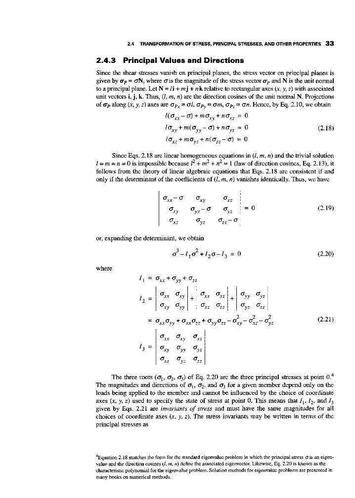
2.4.3 Principal Values and Directions

Since the shear stresses vanish on principal planes, the stress vector on principal planes is given by up = ON, where o i s the magnitude of the stress vector up and N is the unit normal to a principal plane. Let N = l i + mj + n k relative to rectangular axes (x, y, z ) with associated unit vectors i, j , k. Thus, (1, m, n) are the direction cosines of the unit normal N. Projections of up along (x, y, z ) axes are opx = ol, opy = om, opz = on. Hence, by Eq. 2.10, we obtain

+ o x , =xz + o y y o y z

o x z o z z o y z o z z

l ( o x x - o ) + m o x y + n o x z = 0

l o + m ( o - o ) + n o y z = 0

l o x z + m o y z + n ( o z z - o ) = 0 X Y YY

I, =

(2.18)

o x x o x y o x z

OYY O Y Z

o x z o y z =zz

Since Eqs. 2.18 are linear homogeneous equations in (1, m, n) and the trivial solution 1 = m = n = 0 is impossible because l2 + m2 + n2 = 1 (law of direction cosines, Eq. 2.13), it follows from the theory of linear algebraic equations that Eqs. 2.18 are consistent if and only if the determinant of the coefficients of (1, m, n) vanishes identically. Thus, we have

o x x - o x y =xz

OY Z oxy o -0

O X Z OY Z o z z -

= o YY

or, expanding the determinant, we obtain

3 2 o - I , o +120-13 = 0

where I , = oxx+ o + ozz YY

(2.19)

(2.20)

(2.21)

The three roots (q, 02, 03) of Eq. 2.20 are the three principal stresses at point 0.4 The magnitudes and directions of o,, 02, and 0, for a given member depend only on the loads being applied to the member and cannot be influenced by the choice of coordinate axes (x, y, z ) used to specify the state of stress at point 0. This means that I , , I,, and Z, given by Eqs. 2.21 are invariants of stress and must have the same magnitudes for all choices of coordinate axes (x, y, z). The stress invariants may be written in terms of the principal stresses as

4Equation 2.18 matches the form for the standard eigenvalue problem in which the principal stress o i s an eigenvalue and the direction cosines ( I , m, n) define the associated eigenvector. Likewise, Eq. 2.20 is known as the characteristic polynomial for the eigenvalue problem. Solution methods for eigenvalue problems are presented in many books on numerical methods.


I , = 6, + o2 + o3

EXAMPLE 2.1 Principal

Stresses and Principal

Directions

Solution

When (q, o,, 03) have been determined, the direction cosines of the three principal axes are obtained from Eqs. 2.18 by setting d in turn equal to (c~, 9, g), respectively, and observing the direction cosine condition l2 + m2 + n2 = 1 for each of the three values of 0. See Example 2.1.

In special cases, two principal stresses may be numerically equal. Then, Eqs. 2.18 show that the associated principal directions are not unique. In these cases, any two mutually perpendicular axes that are perpendicular to the unique third principal axis will serve as principal axes with corresponding principal planes. If all three principal stresses are equal, then o, = 0, = 0, at point 0, and all planes passing through point 0 are principal planes. In this case, any set of three mutually perpendicular axes at point 0 will serve as principal axes. This stress condition is known as a state of hydrostatic stress, since it is the condition that exists in a fluid in static equilibrium.

The state of stress at a point in a machine part is given by o, = - 10, oyr = 3 0 , ~ = 15, and o, = o,, = oyz = 0; see Figure E2. la. Determine the principal stresses and orientation of the pnncipal axes at the point. a

I f N 1

#35

FIGURE EZ.1

By Eq. 2.21 the three stress invariants are

Substituting the invariants into Eq. 2.20 and solving for the three roots of this equation, we obtain the principal stresses

0, = 35, o2=O0’ and o3 = -15

To find the orientation of the first principal axis in terms of its direction cosines l,, m,, and n,, we substitute o, = 35 into Eq. 2.18 for 0. The direction cosines must also satisfy Eq. 2.13. Thus, we have

-451, + 15ml = 0 (a>

151, -5ml = 0

-359 = 0

2 2 2 l l + m l + n l = 1


Only two of the first three of these equations are independent. Equation (c) gives

nl = 0

Simultaneous solution of Eqs. (b) and (d) yields the result

1; = 0.10 ~

I Z, = k0.3162 i Or

~

I ' Substituting into Eq. (b) for Z,, we obtain

m1 = k0.9487

where the order of the + and - signs corresponds to those of I , . Note also that Eq. (a) is satisfied with these values of Z,, ml, and nl. Thus, the first principal axis is directed along unit vector N1, where

N, = 0.3162i + 0.9487j ; Ox= 71.6" (el or

N, = -0.31623 - 0.9487j

where i and j are unit vectors along the x and y axes, respectively.

which yields The orientation of the second principal axis is found by substitution of o= 9 = 0 into Eq. 2.18,

1, = 0 and m2 = 0

Proceeding as for 0, , we then obtain

n2 = f 1

from which

N2 = fk

where k is a unit vector along the z axis. The orientation of the third principal axis is found in a similar manner:

I , = k0.9487

m3 = ~0.3162

n, = 0

To establish a definite sign convention for the principal axes, we require them to form a right-handed triad. EN, and N, are unit vectors that define the directions of the first two principal axes, then the unit vector N, for the third principal axis is determined by the right-hand rule of vector multiplication. Thus, we have

N, = N , x N ,

or

N, = (mln2-m2nl)i+(12nl-lln2)j+(11m2-12ml)k (8)

In our example, if we arbitrarily select N, from Eq. (e) and N2 = +k, we obtain N, from Eq. (9) as

N, = 0.94871 - 0.3162j

The principal stresses 0, = 35 and 6, = -15 and their orientations (the corresponding principal axes) are illustrated in Figure E2.lb. The third principal axis is normal to the x-y plane shown and is directed outward from the page. The corresponding principal stress is 0, = 0. Since all the stress components associated with the z direction (c,,, ox,, and (T ) are zero, this stress state is said to be a state of plane stress in the x-y plane (see the discussion later in this section on plane stress). yz.

36 CHAPTER z THEORIES OF STRESS AND STRAIN

I 3 =

EXAMPLE 2.2 Stress Invariants

OXX o x y 0 x 2

0 x 2 o y z o z z

cXy cry oZy = -163,000

Solution

The known stress components at a point in a body, relative to the (x, y, z ) axes, are o, = 20 MPa, ow = 10 MPa, oXy = 30 MPa, ox, = -10 MPa, and oyz = 80 MPa. Also, the second stress invariant is I , = -7800

(a) Determine the stress component ozz. Then determine the stress invariants I, and I , and the three principal stresses.

(b) Show that I,, I,, and I , are the same relative to (x, y , z) axes and relative to principal axes (1,2,3).

2.4.4 Octahedral Stress

Let (X, r: Z) be principal axes. Consider the family of planes whose unit normals satisfy the relation Z 2 = m = n = with respect to the principal axes (X, Y; Z). There are eight such planes (the octahedral planes, Figure 2.9) that make equal angles with respect to the (X, X Z) directions. Therefore, the normal and shear stress components associated with these planes are called the octahedral normal stress ooct and octahedral shear stress t&. By Eqs. 2.1G2.12, we obtain


y l

2

FIGURE 2.9 Octahedral plane for I = rn = n = I / & , relative to principal axes (X, K Z).

since for the principal axes oxx = ol, ow = 02, ozz = 03, and om = oyz = om = 0. (See Eqs. 2.21.) It follows that since ( I I , Z2, Z3) are invariants under rotation of axes, we may refer Eqs. 2.22 to arbitrary (x, y, z) axes by replacing I,, Z2, Z3 by their general forms as given by Eqs. 2.21. Thus, for arbitrary (x, y, z) axes,

1 3

ooct = ADxx + oyy + ozz)

(2.23) - 1 2 2 2

The octahedral normal and shear stresses play a role in yield criteria for ductile metals (Section 4.4).

2.4.5 Mean and Deviator Stresses

Experiments indicate that yielding and plastic deformation of ductile metals are essen- tially independent of the mean normal stress om, where

(2.24)

Comparing Eqs. 2.22-2.24, we note that the mean normal stress om is equal to o,,,. Most plasticity theories postulate that plastic behavior of materials is related primarily to that part of the stress tensor that is independent of om. Therefore, the stress array (Eq. 2.5) is rewritten in the following form:

T = Tm+Td (2.25)

where T symbolically represents the stress array, Eq. 2.5, and

om 0 (2.26a)

and

T, =

T, =

(2.26b)


The array T, is called the mean stress tensor. The array Td is called the deviutoric stress tensor, since it is a measure of the deviation of the state of stress from a hydrostatic stress state, that is, from the state of stress that exists in an ideal (frictionless) fluid.

Let (x, y, z) be the transformed axes that are in the principal stress directions. Then,

Oxx = 6,' oyy = 0 2 , Ozz = 03,

and Eq. 2.25 is simplified accordingly. Application of Eqs. 2.21 to Eq. 2.26b yields the following stress invariants for Td:

oxy - - ox. = oyz = 0

J , = 0

J , = i2--i, 1 2 = -1[(01-02) 2 +(02-03) 2 +(4-0,)~] 3 6

1 3 2 7 '

J , = i3 - - i , i + 2i3

= ( 0 1 - 6 m ) ( 6 2 - - ~ ) ( 0 3 - - m )

The principal directions for T, are the same as those for T. It can be shown that since J , = 0, T, represents a state ofpure shear. The principal values of the deviatoric tensor Td are

s, = ol-om =

s, = 0, - om =

s3 = O3 - om =

3 3

Since S, + S, + S, = 0, only two of the principal stresses (values) of T, are independent. Many of the formulas of the mathematical theory of plasticity are often written in terms of the invariants of the deviatoric stress tensor T,.

2.4.6 Plane Stress In a large class of important problems, certain approximations may be applied to simplify the three-dimensional stress array (see Eq. 2.3). For example, simplifying approximations can be made in analyzing the deformations that occur in a thin flat plate subjected to in- plane forces. We define a thin plate to be a prismatic member of a very small length or thickness h. The middle surface of the plate, located halfway between its ends (faces) and parallel to them, may be taken as the (x, y) plane. The thickness direction is then coincident with the direction of the z axis. If the plate is not loaded on its faces, a,, = o,, = oZr = 0 on its lateral surfaces (z = fh/2). Consequently, since the plate is thin, as a first approxima- tion, it may be assumed that

Ozz = Ozx = Ozy = 0 (2.29)

throughout the plate thickness.


We also assume that the remaining stress components o,, oyy, and ov are independent of z . With these approximations, the stress array reduces to a function of the two variables (x, y). It is called a plane stress array or the tensor of plane stress.

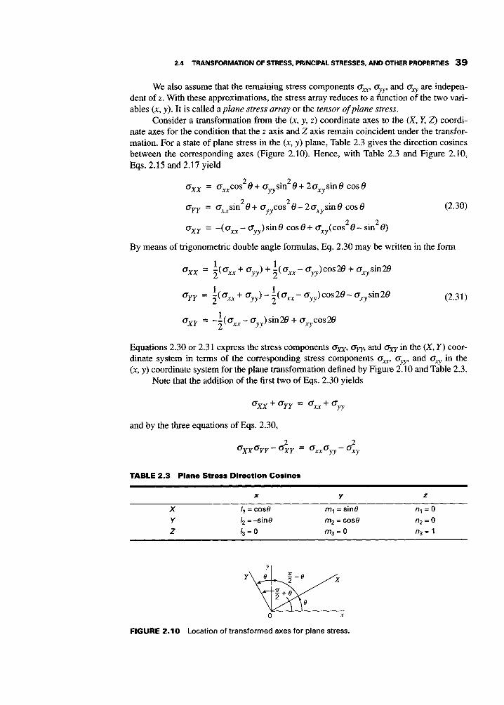
Consider a transformation from the (x, y, z ) coordinate axes to the (X, Y, Z) coordinate axes for the condition that the z axis and 2 axis remain coincident under the transformation. For a state of plane stress in the (x, y) plane, Table 2.3 gives the direction cosines between the corresponding axes (Figure 2.10). Hence, with Table 2.3 and Figure 2.10, Eqs. 2.15 and 2.17 yield

2 2 oxx = o,,COS e + oyYsin e + 2oXy sin e cos e oyy = oxxsin 2 8 + oyycos 2 8- 2oXysin8 cos 8 (2.30)

2 2 oxY = -( oxx - oyy ) sin 8 cos 8 + oxy( cos 8 - sin 8)

By means of trigonometric double angle formulas, Eq. 2.30 may be written in the form

oXx = -( 1 oxx + o ) + -( 1 oxx - oyy) cos2B + oxy sin28

oyy = - (oxx+o 1 ) - - (oxx-o 1 )cos28-oxysin28

oxy = --( 1 oxx - oyy) sin28 + oxycos2B

2 yy 2

2 yy 2 YY

2

(2.31)

Equations 2.30 or 2.31 express the stress components om, o,, and om in the (X, Y) coordinate system in terms of the corresponding stress components o,, oyy, and oxr in the (x, y ) coordinate system for the plane transformation defined by Figure 2.10 and Table 2.3.

Note that the addition of the first two of Eqs. 2.30 yields

and by the three equations of Eqs. 2.30,

2 2 oxxoyv - O X Y = o x x o y y - o x y

TABLE 2.3 Plane Stress Direction Cosines

X Y z

X 1, = case m, = sin6 n1 = 0 Y l2 = -sin6 m2 = cose n2 = 0 Z l3 = 0 m 3 = 0 n3 = 1

0 X

FIGURE 2.10 Location of transformed axes for plane stress.


Hence, the stress invariants for a state of plane stress are

2.4.7 Mohr’s Circle in Two Dimensions

In the form of Eq. 2.31, the plane transformation of stress components is particularly suited for graphical interpretation. Stress components oxx and om act on face BE in Fig- ure 2.11 that is located at a positive (counterclockwise) angle 8 from face BC on which stress components o, and o act. The variation of the stress components om and om with 8 may be depicted graphically by constructing a diagram in which oxx and om are coordinates. For each plane BE, there is a point on the diagram whose coordinates corre- spond to values of oxx and om

Rewriting the first of Eqs. 2.31 by moving the first term on the right side to the left side and squaring both sides of the resulting equation, squaring both sides of the last of Eq. 2.3 1, and adding, we obtain

xr

(2.32)

Equation 2.32 is the equation of a circle in the om, om plane whose center C has coordinates r 1

and whose radius R is given by the relation

R = l m y

(2.33)

(2.34)

Consequently, the geometrical representation of the first and third of Eqs. 2.31 is a circle (Figure 2.12). This stress circle is frequently called Mohr’s circle after Otto Mohr, who employed it to study plane stress problems. It is necessary to take the positive direction of the oxu axis downward so that the positive direction of 8 in both Figures 2.1 1 and 2.12 is counterclockwise.

FIGURE 2.1 1 stress.

Stress components on a plane perpendicular to the transformed Xaxis for plane


FIGURE 2.12 Mohr‘s circle for plane stress.

Since o,, oyy, and oxy are known quantities, the circle in Figure 2.12 can be constructed using Eqs. 2.33 and 2.34. The interpretation of Mohr’s circle of stress requires that one known point be located on the circle. When 8 = 0 (Figure 2. lo), the first and third of Eqs. 2.3 1 give

oXx = oXx and oxY = oXy (2.35)

which are coordinates of point P in Figure 2.12. Principal stresses ol and o. are located at points Q and Q’ in Figure 2.12 and occur

when 6 = and 6, + ~ 1 2 , measured counterclockwise from line CP. The two magnitudes of 8 are given by the third of Eqs. 2.3 1 since o, = 0 when 8 = and 8, + ~ 1 2 . Note that, in Figure 2.12, we must rotate through angle 28from line CP, which corresponds to a rotation of 8 from plane BC in Figure 2.11. (See also Eqs. 2.31.) Thus, by Eqs. 2.31, for ox, = 0, we obtain (see also Figure 2.12)

2o.y *xx - oyy

tan28 = (2.36)

Solution of Eq. 2.36 yields the values 8 = 8, and 8, + ~ 1 2 .

in the (x, y) plane from Mohr’s circle are The magnitudes of the principal stresses ol, o2 and the maximum shear stress z,,,

(2.37)

and are in agreement with the values predicted by the procedure outliied earlier in this section. Another known point on Mohr’s circle of stress can be located, although it is not needed

for the interpretation of the circle. When 8 = ~ 1 2 , the first and third of Eqs. 2.31 give

oXX = oYY and oxy=-oXy (2.38)

These coordinates locate point P’ in Figure 2.12, which is on the opposite end of the diam- eter from point P.

Note that Example 2.1 could also have been solved by means of Mohr’s circle.


EXAMPLE 2.3 Mohr's Circle in

Two Dimensions

Solution

A piece of chalk is subjected to combined loading consisting of a tensile load P and a torque T (Figure E2.3~). The chalk has an ultimate strength 0, as determined in a simple tensile test. The load P remains constant at such a value that it produces a tensile stress 0.510, on any cross section. The torque T is increased gradually until fracture occurs on some inclined surface.

Assuming that fracture takes place when the maximum principal stress 0, reaches the ultimate strength o,, determine the magnitude of the torsional shear stress produced by torque T at fracture and determine the orientation of the fracture surface.

Take the x and y axes with their origin at a point on the surface of the chalk as shown in Figure E2.32. Then a volume element taken from the chalk at the origin of the axes will be in plane stress (Figure E2.27) with ou = 0.5 1 o,, oyy = 0, and 0- unknown. The magnitude of the shear stress 0- can be determined from the condition that the maximum principal stress 0, (given by Eq. 2.37) is equal to 0,; thus,

0, = 0.2550, + ,,/wv ox. = 0.7000,

Since the torque acting on the right end of the piece of chalk is counterclockwise, the shear stress 0- acts down on the front face of the volume element (Figure E2.3b) and is therefore negative. Thus,

Oxy = -0.7000"

In other words, 0- actually acts downward on the right face of Figure E2.3b and upward on the left face. We determine the location of the fracture surface first using Mohr's circle of stress and then using Eq. 2.36. As indicated in Figure E2.3c, the center C of Mohr's circle of stress lies on the oXx axis at dis- tance 0.2550, from the origin 0 (see Eq. 2.33). The radius R of the circle is given by Eq. 2.34; R = 0.7450,. When 6 = 0, the stress components Oxx(6 = o) = 0, = 0.5 lo, and ox,, = o) = oq = -0.7000, locate point

t ax,

FIGURE E2.3

.70mu

C - - - u a l = u " 4


P on the circle. Point Q representing the maximum principal stress is located by rotating clockwise through angle 28, from point P; therefore, the fracture plane is perpendicular to the X axis, which is located at an angle 8, clockwise from the x axis. The angle 8, can also be obtained from Q. 2.36, as the solution of

2(0.7000u) 0.5 1 o,

tan 28 - 2oxY - = -2.7451 I - - - - oxx

Thus,

8, = -0.6107 rad

Since 8, is negative, the X axis is located clockwise through angle 8, from the x axis. The fracture plane is at angle @ from the x axis. It is given as

7T @ = --/8,1 = 0.9601 rad

The magnitude of @ depends on the magnitude of P. If P = 0, the chalk is subjected to pure torsion and @ = n/4. If P / A = o, (where A is the cross-sectional area), the chalk is subjected to pure tension (T = 0) and 4 = ~ / 2 .

2

2.4.8 Mohr‘s Circles in Three Dimensions5

As discussed in Chapter 4, the failure of load-carrying members is often associated with either the maximum normal stress or the maximum shear stress at the point in the member where failure is initiated. The maximum normal stress is equal to the maximum of the three principal stresses o,, 02, and 0,. In general, we will order the principal stresses so that o, > o2 > 0,. Then, o, is the maximum (signed) principal stress and 0, is the minimum principal stress (see Figure 2.13.) Procedures have been presented for determining the values of the principal stresses for either the general state of stress or for plane stress. For plane stress states, two of the principal stresses are given by Eqs. 2.37; the third is o, = 0.

Even though the construction of Mohr’s circle of stress was presented for plane stress (ozz = 0), the transformation equations given by either Eqs. 2.30 or 2.31 are not influenced by the magnitude of o,, but require only that ozx = ozy = 0. Therefore, in terms

uNS

FIGURE 2.13 Mohr’s circles in three dimensions.

’In the early history of stress analysis, Mohr’s circles in three dimensions were used extensively. However, today they are used principally as a heuristic device.

4 4 CHAPTER 2 THEORIES OF STRESS AND STRAIN

of the principal stresses, Mohr's circle of stress can be constructed by using any two of the principal stresses, thus giving three Mohr's circles for any given state of stress. Consider any point in a stressed body for which values of ol, 02, and o3 are known. For any plane through the point, let the N axis be normal to the plane and the S axis coincide with the shear component of the stress for the plane. If we choose 0" and oNS as coordinate axes in Figure 2.13, three Mohr's circles of stress can be constructed. As will be shown later, the stress components 0" and oNS for any plane passing through the point locate a point either on one of the three circles in Figure 2.13 or in one of the two shaded areas. The maximum shear stress z,, for the point is equal to the maximum value of oNS and is equal in magnitude to the radius of the largest of the three Mohr's circles of stress. Hence,

(2.39)

where a,, = ol and omin = o3 (Figure 2.13). Once the state of stress at a point is expressed in terms of the principal stresses, three

Mohr's circles of stress can be constructed as indicated in Figure 2.13. Consider plane P whose normal relative to the principal axes has direction cosines 1, m, and n. The normal stress oNN on plane P is, by Eq. 2.11,

(2.40) 2 2 2 oNN = 1 o l + m 0 2 + n o3

Similarly, the square of the shear stress oNS on plane P is, by Eqs. 2.10 and 2.12,

(2.41) 2 2 2 2 2 2 2 2 oNs = 1 o l + m 0 2 + n 0 3 - 0 "

For known values of the principal stresses ol, 02, and o3 and of the direction cosines 1, m, and n for plane P, graphical techniques can be developed to locate the point in the shaded area of Figure 2.13 whose coordinates (o", oNS) are the normal and shear stress components acting on plane P. However, we recommend the procedure in Section 2.3 to determine magnitudes for 0" and oNS. In the discussion to follow, we show that the coordinates (0". oNS) locate a point in the shaded area of Figure 2.13.

Since

(2.42) 2 2 2 1 + m + n = 1

Eqs. 2.40-2.42 comprise three simultaneous equations in 12, m2, and n2. Solving for 12, m2, and n2 and noting that l2 2 0, m2 2 0, and n2 2 0, we obtain

2 2 ON,$ + ( O N N - O 2 ) ( O N N - O3) 2 0 I =

(01 - q(o1 - 0 3 )

(2.43)

Ordering the principal stresses such that ol > o2 > 0 3 , we may write Eqs. 2.43 in the form


EXAMPLE 2.4 Mohr‘s Circles

in Three Dimensions

Solution

These inequalities may be rewritten in the form

(2.44)

where 7, = $ 19 - O, I , 7, = 1 10, - O, I , = 1 10, - 0, I are the maximum (extreme) magnitudes of the shear stresses in three-dimensional principal stress space and (o~, o,, 03) are the signed principal stresses (see Figure 2.13). The inequalities of Eqs. 2.44 may be inter- preted graphically as follows: Let (o“, oNS) denote the abscissa and ordinate, respectively, on a graph (Figure 2.13). Then, an admissible state of stress must lie within a region bounded by three circles obtained from Eqs. 2.44 where the equalities are taken (the shaded region in Figure 2.13).

The state of stress at a point in a machine component is given by a, = 120 MPa, oYY = 55 MPa, o,, = -85 MPa, a- = -55 MPa, ox, = -75 MPa, and oY2 = 33 MPa. Construct the Mohr’s circles of stress for this stress state and locate the coordinates of points A: (““I, aNSl) and B: (““2, “NS2) for normal and shear stress acting on the cutting planes with outward normal vectors given by N, : ( 1 / b , l /&, 1b) and N2 : ( l / , h , l /&, 0) relative to the principal axes of stress.

Substituting the given stress components into Eq. 2.20, we obtain

0~-900‘-18,014~~+471,680 = 0

The three principal stresses are the three roots of this equation. They are

c1 = 176.80 MPa, o2 = 24.06 MPa, 0, = -110.86 MPa

The center and radius of each circle is found directly from the principal stresses as

“2 - “3

C 2 : ( “ 1 i “ 3 , 0 ) = (32.97MPa,O),

C, : ( 9 . 0 ) = (100.43 MPa, 0),

“1 - “3 R, = = 143.83 MPa

“1 - “2 R, = = 76.37 MPa

Figure E2.4 illustrates the corresponding circles with the shaded area indicating the region of admissible stress states. The normal and shear stresses acting on the planes with normal vectors N, and N2 are found from Eqs. 2.40 and 2.41:

oNN1 = 30 MPa, oNs, = 117.51 MPa Point A,

oNN2 = 100.43 MPa, oNs2 = 76.37 MPa Point €3;


EXAMPLE 2.5 Three

Dimensional Stress Quantities

Solution

These points are also shown in Figure E2.4. By this method, the correct signs of oNsl and oNs2 are inde- terminate. That is, this method does not determine if oNs, and oNs2 are positive or negative. They are plotted in Figure E2.4 as positive values. Note that, since N2 : (l/.&, 1/.&, 0), the third direction cosine is zero and point B lies on the circle with center C3 and radius R,.

ONS

FIGURE E2.4

At a certain point in a drive shaft coupling, the stress components relative to axes (x, y, z) are o, = 80 MPa, oyy = 60 MPa, o,, = 20 MPa, oxy = 20 MPa, ox, = 40 MPa, and oyz = 10 MPa.

(a) Determine the stress vector on a plane normal to the vector R = i + 2j + k. (b) Determine the principal stresses o,, 02, and o3 and the maximum shear stress z,,,.

(e) Determine the octahedral shear stress T,,, and compare it to the maximum shear stress.

(a) The direction cosines of the normal to the plane are

By Eqs. 2.10, the projections of the stress vector are

(80) + - (20) + - (40) = 65.320 MPa opx=[i) (4 (4 opy = ( i ) ( 2 0 ) + ( 2 ) ( 6 O ) + [ i ) ( l O ) = 61.237 MPa

(20) = 32.660 MPa

Hence,

up = 65.3203 + 61.2371 + 32.660k

(b) For the given stress state, the stress invariants are (by Eq. 2.21)

I , = ~ x x x + ~ y y + b z z = 160


I 3 =

EXAMPLE 2.6 Stress in a

Torsion Bar

Oxx %y Oxz

0 x 2 0 y z 0 2 2

Ox)) Oyy OY2 = 0

Solution

Comparing z,,, and z ~ ~ ~ , we see that

zmax = 1 . 2 2 3 ~ ~ ~ ~

The stress array for the torsion problem of a circular cross section bar of radius u and with longitudi- nal axis coincident with the z axis of rectangular Cartesian axes (x, y , z) is

0 0 -Gyp T = [ 0 0 G i P ] (a>

-GYP GxP

where G and pare constants (see Figure E2.6).

(a) Determine the principal stresses at a point x = y on the lateral surface of the bar.

(b) Determine the principal stress axes for a point on the lateral surface of the bar.

FIGURE E2.6

(a) For a point on the lateral surface of the bar, u2 = x2 + y2 (Figure E2.6). Then, by Eq. (a),

2 2 2 I , = O , 1 2 = - G p a , I 3 = 0


Hence, the principal stresses are the roots of

o3 + I ,O = o3 - G2p2a20 = o

So the principal stresses are

o1 = Gpa, 02= 0, o3 =&pa

(b) For the principal axis with direction cosines I, m, and n corresponding to o,, we substitute o, = Cpa into Eq. 2.18 for o. Hence, the direction cosines are the roots of the following equations:

I l ( a x x - o l ) + m o + n l o x z = 0

I 1 (T XY + m l ( o y y - ~ l ) + n l o y y r = 0 1 X Y

1 , OXZ + m1 oyz + n1 (oz7 - 0,) = 0 2 2 2 I l + m l + n l = 1.0

where, since x = y = a f A is a point on the lateral surface,

OXX = oyy = ozz = oxy = 0

- - -- CPa A 0 x 2 = -GyPIy=

- - - CPa oYZ = Gx’lx= a / A A

-I1-- “1 = o j 1 1 = - 2 A A

A l-3

-- ‘1 +?-n, = 0

By Eqs. (b), (c), and 2.13, we obtain

n

nl nl - m l + - = O j m -

A A 2 2 2 2 I I + m l + n l = 2nl = 1.0

Therefore,

1 1 1 n l = _+- I , = T ~ , m1 = kZ A’

So, the unit vector in the direction of ol is

( 4 1 1 1 N = T-i _+ -j -k

l 2 2 2 / 2

where i, j, k are the unit vectors in the positive senses of axes (x, y , z), respectively. Similarly, for o2 and 03, we find

1 1 N2 = +-i k -j

(e) & A

- +l. 1. 1

A - - Z ~ T z~ k -k


EXAMPLE 2.7 Design

Specifications for an Airplane Wing Member

Solution

The unit vectors N,, N,, N, determine the principal stress axes on the lateral surface for x = y = a/ f i .

apply to any point on the lateral surface of the bar. Note: Since axes x, y may be any mutually perpendicular axes in the cross section, Eqs. (d) and (e)

In a test of a model of a short rectangular airplane wing member (Figure E2.7a), the member is subjected to a uniform compressive load that produces a compressive stress with magnitude 0,. Design specifications require that the stresses in the member not exceed a tensile stress of 400 MPa, a compressive stress of 560 MPa, and a shear stress of 160 MPa. The compressive stress 0, is increased until one of these values is reached.

(a) Which value is first attained and what is the corresponding value of GO?

(b) Assume that 0, is less than 560 MPa. Show that 0, can be increased by applying uniform lateral stresses to the member (Figure E2.7b), without exceeding the design requirements. Determine the values of 0, and oyy to allow 0, to be increased to 560 MPa.

(4

FIGURE E2.7

(a) Since the stress state of the member is uniform axial compression in the z direction, the tensile stress limit will not be reached. However, the shear stress limit might control the design. By Eq. 2.39, the maximum shear stress is given by

(a) 1 zmax = +Omax-Omin)

By Figure E2.7a. 0, = oyy = oXy = oxz = oyz = 0, and ozz = -ow Hence, om, = 0 and omi, = -00.

Therefore, with z,, = 160 MPa, Eq. (a) yields

0, = 320MPa

Thus, the shear stress limit is reached for 0, = 320 MPa.

(b) By Figure E2.7b, the member is subjected to uniform uniaxial stresses in thex, y, and z directions. Hence, the principal stresses are

o1 = OXX, 0, = Ory, 0, = o,, = -0, (b)

Then, by Eqs. (b) and 2.44 and Figure 2.13, the extreme values of the shear stresses are given by 1

1

1

71 = 2 ( 0 2 - 0 3 )

72 = 2(0' - 03)

73 = p1 - 0 2 )

50 CHAPER 2 THEORIES OF STRESS AND STRAIN

For shear stress to control the design, one of these shear stresses must be equal to 160 MPa. We first consider the possibility that 7, = 160 MPa. Since o,, = -0, and o0 is a positive number, Eqs. (b) and the first of Eqs. (c) yield

00 = 320 - 02 (4

Next we consider the possibility that z2 = 160 MPa. By Eqs. (b) and the second of Eqs. (c), we find

00 = 320 - 01 (el

For 6, = 0, = 0, Eqs. (d) and (e) yield o0 = 320 MPa, as in part (a). Also note that, for O, and o2 negative (compression), Eqs. (d) and (e) show that o0 can be increased (to a larger compressive stress) without exceeding the requirement that z,,, not be larger than 160 MPa. Finally note that, for o0 = 560 MPa (560 MPa compression), Eqs. (d) and (e) yield

o1 = a2 = -240 MPa

2.5 DIFFERENTIAL EQUATIONS OF MOTION OF A DEFORMABLE BODY

In this section, we derive differential equations of motion for a deformable solid body (differential equations of equilibrium if the deformed body has zero acceleration). These equations are needed when the theory of elasticity is used to derive load-stress and load- deflection relations for a member. We consider a general deformed body and choose a differential volume element at point 0 in the body as indicated in Figure 2.14. The form of the differential equations of motion depends on the type of orthogonal coordinate axes employed. We choose rectangular coordinate axes (x, y, z) whose directions are parallel to the edges of the volume element. In this book, we restrict our consideration mainly to small displacements and, therefore, do not distinguish between coordinate axes in the deformed state and in the undeformed state (Boresi and Chong, 2000). Six cutting planes bound the volume element shown in the free-body diagram of Figure 2.15. In general, the state of stress changes with the location of point 0. In particular, the stress components undergo changes from one face of the volume element to another face. Body forces (Bx, By, B,) are included in the free-body diagram. Body forces include the force of grav- ity, electromagnetic effects, and inertial forces for accelerating bodies.

t FIGURE 2.14 General deformed body.

2.5 DIFFERENTIAL EQUATIONS OF MOTION OF A DEFORMABLE BODY 5 1

FIGURE 2.15 Stress components showing changes from face to face along with body force per unit volume including inertial forces.

To write the differential equations of motion, each stress component must be multiplied by the area on which it acts and each body force must be multiplied by the volume of the element since (B,, By, B,) have dimensions of force per unit volume. The equations of motion for the volume element in Figure 2.15 are then obtained by summation of these forces and summation of moments. In Section 2.3 we have already used summation of moments to obtain the stress symmetry conditions (Eqs. 2.4). Summation of forces in the x direction gives6

do,, J o y , do,, - + - + - + B, = 0 dx ay m where on, or, = oxr, and ox, = 0, are stress components in the x direction and B, is the body force per unit volume in the x direction including inertial (acceleration) forces. Sum- mation of forces in the y and z directions yields similar results. The three equations of motion are thus

+ B , = 0 do,, day, do,,

d o x y do,, d o z y & ay A + B Y = o

do,, J o y . do,, - + - + - + B , = 0 dx ay m

- + - + - dx ay &

- + - + - (2.45)

As noted earlier, the form of the differential equations of motion depends on the coordinate axes; Eqs. 2.45 were derived for rectangular coordinate axes. In this book we also need differential equations of motion in terms of cylindrical coordinates and plane

6Note that a, on the left face of the element goes to o, + do, = o, + (aa,/dx)d* on the right face of the element, with similar changes for the other stress components (Figure 2.15).


polar coordinates. These are not derived here; instead, we present the most general form from the literature (Boresi and Chong, 2000, pp. 204-206) and show how the general form can be reduced to desired forms. The equations of motion relative to orthogonal curvilinear coordinates (x, y, z) (see Figure 2.16) are

d(P.yoxx> J (Yaoyx> + d(aPo,,) da + YOyx- dr dZ dr +

dX

(2.46)

ao d p + a P y B , = 0 yy dz

where (a, P, y ) are metric coefficients that are functions of the coordinates (x, y, z) . They are defined by

(2.47) 2 2 2 2 2 2 2 d s = a d x + P d y + y d z

where ds is the differential arc length representing the diagonal of a volume element (Fig- ure 2.16) with edge lengths a &, P dy, and ydz, and where (Bx, By, B,) are the components of body force per unit volume including inertial forces. For rectangular coordinates, a = P = y= 1 and Eqs. 2.46 reduce to Eqs. 2.45.

2.5.1 Specialization of Equations 2.46

Commonly employed orthogonal curvilinear systems in three-dimensional problems are the cylindrical coordinate system (r, 8, z ) and spherical coordinate system (r, 8, $); in plane problems, the plane polar coordinate system (r, 8) is frequently used. We will now specialize Eqs. 2.46 for these systems.

(a) Cylindrical Coordinate System (r, 6, z). In Eqs. 2.46, we let x = r, y = 8, and z = z. Then the differential length ds is defined by the relation

ds2 = dr2 + r 2 d 8 + dz2 (2.48)

a&

FIGURE 2.16 Orthogonal curvilinear coordinates.

Next Page

2.5 DIFFERENTIAL EQUATIONS OF MOTION OF A DEFORMABLE BODY 53

A comparison of Eqs. 2.47 and 2.48 yields

a = l , P = r , y = l (2.49)

Substituting Eq. 2.49 into Eqs. 2.46, we obtain the differential equations of motion

+ B , = 0 ' o r , I'o~, d o z y o r r - 0 8 8 -+--+-+ dr r d 8 dz r

(2.50)

where (err, 060, o,,, Ore, o,, GOz) represent stress components defined relative to cylindrical coordinates (r, 8, z). We use Eqs. 2.50 in Chapter 11 to derive load-stress and load- deflection relations for thick-wall cylinders.

(b) Spherical Coordinate System (4 8, @). In Eqs. 2.46, we let x = r, y = 8, and z = @, where r is the radial coordinate, 8 is the colatitude, and Cp is the longitude. Since the differential length ds is defined by

ds2 = dr2 + r2d82 + r2sin28 d@2 (2.51)

comparison of Eqs. 2.47 and 2.51 yields

a = 1, p = r, y = rs in8 (2.52)

Substituting Eq. 2.52 into Eqs. 2.46, we obtain the differential equations of motion

3 + 1 8 0 , - - + - ( 3 a , g + 2 0 do 1 a*,, 1 cote)+Bo = o dr r d8 rsin8 dCp r ee

where (err, oee, ooc Ore, or+ oe4) are defined relative to spherical coordinates (r, 8, @).

(c) Plane Polar Coordinate System (r, 8). In plane-stress problems relative to (x, y) coordinates, o,, = ox, = oyz = 0, and the remaining stress components are functions of (x, y) only (Section 2.4). Letting x = r, y = 8, and z = z in Eqs. 2.50 and noting that o,, = or, = o, = (d/aZ) = 0, we obtain from Eq. 2.50, with a= 1, p = r, and y= 1,

(2.54)

Previous Page


2.6 DEFORMATION OF A DEFORMABLE BODY

In this and the next section we consider the geometry of deformation of a body. First we examine the change in length of an infinitesimal line segment in the body. From that, finite strain-displacement relations are derived. These are then simplified according to the assumptions of small-displacement theory. Additionally, differential equations of compatibility, needed in the theory of elasticity, are derived in Section 2.8.

In the derivation of strain-displacement relations for a member, we consider the member first to be unloaded (undeformed and unstressed) and next to be loaded (stressed and deformed). We let R represent the closed region occupied by the undeformed member and R* the closed region occupied by the deformed member. Aster- isks are used to designate quantities associated with the deformed state of members throughout the book.

Let (x, y, z) be rectangular coordinates (Figure 2.17). A particle P is located at the general coordinate point (x, y, z ) in the undeformed body. Under a deformation, the particle moves to a point (x*, y*, z*) in the deformed state defined by the equations

x* = x*(x, y, z)

Y* = Y*(X, y, z ) (2.55)

z* = z*(x, y, 2 )

where the values of (x, y, z ) are restricted to region R and (x*, y*, z*) are restricted to region R*. Equations 2.55 define the final location of a particle P that lies at a given point (x, y, z) in the undeformed member. It is assumed that the functions (x*, y*, z*) are continuous and differentiable in the independent variables (x, y, z), since a discontinuity of these functions would imply a rupture of the member. Mathematically, this means that Eqs. 2.55 may be solved for single-valued solutions of (x, y, z); that is,

x = x(x*,y*,z*)

y = Y(X*, Y*, 2")

z = z(x*,y*,z*)

(2.56)

Equations 2.56 define the initial location of a particle P that lies at point (x*, y*, z*) in the deformed member. Functions (x, y, z ) are continuous and differentiable in the independent variables (x*, y*, z*).

y 3 q,. ;*- . , ,

FIGURE 2.17 Location of general point Pin undeformed and deformed body.

Documents

CHAPTER THEORIES OF STRESS AND STRAIN